Estimating Wind Speed In Black Sea Region With Panel Data Analysis

ESTIMATING WIND SPEED IN BLACK SEA REGION WITH PANEL DATA ANALYSIS

Zeynep ATLI1_{, Alper SİNAN}1

1_{Sinop University Science and Agriculture Faculty, Department of Statistics,}

Sinop-Turkey, zatli@sinop.edu.tr, alpsin@sinop.edu.tr

ABSTRACT

Panel data analysis is a common method used especially in economic research and in other research in which time/unit relationship is significant. This study aims at predicting average wind speed during the years 2009-2010 in the cities of Sinop, Samsun, Ordu, Kastamonu, Bartın, Zonguldak and Karabük of Blacksea Region. In order to analyze the obtained data, of all panel data analysis methods, Random Effect Model and Fixed Effect Model have been used. Compatibility of these data sets have been compared via the use of graphics. The results have shown that Fixed Effect Model has turned out to be more effective in analyzing data according to units.

Key Words: Panel data, Random Effects Model, Wind speed, Fixed Effect Model

1. INTRODUCTION

Three types of data that can be used in econometrics research are time series, cross section and pooled data (Gujarati 2004). Time series is a set of observations that a variable takes a value in different times. Cross section refers to a data set that belongs to one or more variables at a single time point. Pooled data is an element of both time series and cross section data. Panel data is a special type of pooled data and panel data set refers to a data set has a data on cross section units over the time.

Panel data has some advantages over cross sectional and time series data. Panel data controls for individual heterogeneity. Time series and cross sectional studies don’t control the heterogeneity. Time series models and cross sectional models which are not controlled the heterogeneity, run the risk of obtaining biased result (Baltagi 2005). Panel data has large number of observation over time series and cross sectional data. Increasing the number of observation increase degrees of freedom. Since explanatory variable vary over both time dimension and cross sectional dimension, multicollinearity

reduce among explonarity variables in panel data. Increasing the degrees of freedom and reducing the multicollinearity, enhance the efficient of estimation (Tüzüntürk 2000).

2. REGRESSION MODELS FOR PANEL DATA

Panel data models have two dimensions on its variables differently from cross sectional and time series. Panel regression model can be written as

1, , 1, , it it kit kit it

y  x  u i  N t  T ₍₁₎

where i donates units, t donates the time dimension, y is the observation on theit dependent variable for i-th individual and t-th time period,it is the intercept varying over time and units. it is the slope coefficient ,xkit is the observation on the independent variable for i-th units and t-th time period. u is the error term. In thisit model all coefficient vary over units and time. The number of parameter to be estimated exceed the observation hence this model cannot estimate. Panel data models can be classified further, depending on whether the coefficients are assumed random or fixed (Hsiao 2003).

2.1.Fixed Effect Models

One way to incorporate for individual or time differences behavior is assumed that some of the regression coefficient or all of them are allowed to vary across individual or over time. (Hsiao 2003). The coefficients are allowed to vary time or / and individual, these models referred to fixed effects model.

In individual effect models we assumed that slope coefficient is constant over time and individuals however intercept is allowed to vary from individual to individual (Màtyàs and Sèvèstrè 2008). This case can be modeled as

1, , 1, , it i kit k it

y  x  u i  N t  T ₍₂₎

i , donates units , t donates time period, x is thekit it-th observation ok k explanatory

variables. y is the value of the dependent variable for i -th units and t -th time.it u isit error term that is assumed to be identically and independently distributed with zero mean and constant variance (u ~ . . . (0, )). In order to make difference among individuals, N dummy variables are added the model. Model can be written matrix notation as

y D  Xu=Z u (3)

where y is anNT x1 vector, X is an NT x q matrix of explanatory variable, u is anit

1

NT x vector of error terms and  is a qx1 vector and  is an N x1 vector.

[ ]

Z  D X _and[ ]_. D is an NT x N matrix of dummy variable and has the following Kronocker product representation,

D=IN ıT (4)

where IN denotes N N identity matrix and ı is a vector of ones of dimension T. ThisT model also referred to as the least squares dummy variable model (LSDV). This model is a classical regression model and if N is small we can estimate the model by ordinary least squares with q regressor in X and N columns in D (Greene 2003). But if N is large, inverting a matrix of (N q ) (N q ) dimension is difficult and this might be a

problem and to avoid this problem partitioned regression can be used (Roy 1997). Using the dummy variable matrix D, one can obtain transform matrix

where 1 ( ' ) ' N NT M _I _D D D D (5) And by using the transform matrixM , we can obtain OLS estimator of N

1

ˆ _{( ' ) ( ' )}

SE X M XN X M YN

 _ 

(6) And intercept term for each i

. . 1 ˆ ˆ_{i i} q _{ki kSE} k Y x     



2 1 ˆ ( ) ( ' N ) Var  _ X M X  (8) 2 . . 1 _ˆ ˆ ( ) ( _i ( ) _i) Var X Var X T    (9) One can test to see whether there is a difference between individual. In this case the null hypothesis is that there is no difference between individuals.

0 1 2 1 1 2 : : N N H H              

Let HKT be the sum of squared residuals obtained from restricted model and1 HKT be2

the sum of squared residuals obtained from unrestricted model. One can use the F test with (N-1) and (NT-N-K) degrees of freedom.

1 2 2 ( 1) ( ) HKT HKT N F HKT NT N K     

If F ratio is larger than the critical value of F, null hypothesis will be rejected. Thus one can decided to units are homogeneity.

In time effects model, assumed that intercept term vary over the time period. Time effects model written as,

1, , 1, , it t kit k it

y   x  u i  N t  T ₍₁₀₎

t

 is a intercept term which is constant over time. The model can be written as matrix notation,

T

y D X u ₍₁₁₎

Where D is a NT x T matrix of time dummies andT  is T x 1 vector of varying intercept.

In time effect models obtaining the parameter estimation resemble by fixed effect models. One can be used partitioned regression to obtain the parameter estimator. Transform matrix in time effect model,

' 1 '

( )

T NT T T T T M _I _D D D  D

(12) Estimation of parameter is exactly the same with fixed effect.

2.2.Random effects models

In fixed effects models the individual-varying variables represented by i and it is possible to indicate over individual-varying in random effect models. If one considered that error term u represents to unobservable effects and omitted variable that vary overit individuals and over time,



it i it

v   u

and we assumed that i and u ,it

3. iis independent and identically distributed with zero mean and  .2 i iid(0, ) .2 4. uit is independent and identically distributed with zero mean and  .2

2 (0, ) it u iid  . 5. E(i itu ) 0 6. E(iXit) 0 and (E u Xit it) 0 Random effect model can be written as,

1, , 1, , it kit k it

y   x  v i  N t  T ₍₁₃₎

And the model rewriting in matrix form,

Where  is q x 1 vector, X is (NT k )design matrix, v is (NT1) error term. µ represents mean intercept.

The parameter of model can be estimated by using generalized least square in random effects model since GLS estimators are the best linear unbiased (BLUE) estimators. The variance covariance matrix of error term v isi

2 2 '

u T T T

V  I _ı ı ₍₁₅₎

The inverse of variance covariance matrix V can be written as

2 1 ' 2 2 T T T u V I ı ı T       _ _   _   

By using equations (18),  estimator can be obtained,ˆ

1 1 1

ˆ_{GEKK ( 'X V X) ( 'X V Y)}

 _   

(16) Mean intercept can be expressed,

.. ˆ ..

ˆ y _REX

  ₍₁₇₎

In order to get inverse of variance covariance matrix of V, one should be compute the estimators of 2



 and 2

u

 . Suggested estimator by Swamy and Arora (1972) for 2

  and 2 u  as follows, 2 . . 2 1 1 ˆ ( ) ˆ ( 1) N T it i kit ki SE i t u y y x x N T q              



2 . . 2 1 2 ˆ ˆ ( ) ₁ ˆ ˆ ( 1) N i G i G i u y x N q T            



where ˆG refers to between groups estimators and is given as,

1 . .. . .. . .. . .. 1 1 ˆ_G T _{( ki )'( ki )} N _{( ki )'( i )} t i x x x x x x y y         _   _{ }   _ 





Breusch and Pagan (1979) suggested using Lagrange Multiplier to test for random effects model. To check for absence of individual effects, the null hypothesis and alternative hypothesis are given as

2 0 2 1 : 0 : 0 H H      

The LM test statistics is written as,

2 1 1 2 1 1 ˆ ( ) 1 2( 1) _{( )ˆ} N T it i t N T it i t v NT LM T  _v                 

 



statistics computed from OLS regression residuals is larger than critical value of _2 _the

3. APPLICATION

This study aims at predicting average wind speed during the years 2009-2010 in the cities of Sinop, Samsun, Ordu, Kastamonu, Bartın, Zonguldak and Karabük of Blacksea Region. Wind speed is a dependent variable, the average minimum temperature; the average maximum temperature and the average humidity are independent variables.

First of all, individual effects are analyzed for fixed effects model. Only individual effects model is written as,

1 1 2 2 3 3 1, ,7 1, ,8

it i it it it

Y  x  x  x  i  t  ₍₂₁₎

Computed value of i for each city and the slope coefficient ˆk which is the same over units, given as in Table 1.

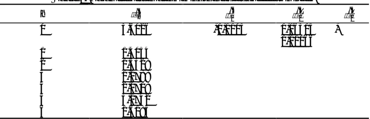
Table 1. Parameter estimation in only individual effects model.

i ˆi ˆ1 ˆ2 ˆ3 1 4,7137 -0,0014 0,07406 -0,02177 2 2,5165 3 2,6439 4 2,3899 5 3,1809 6 4,2853 7 2,7096

In Table 1. ˆ and  estimation is shown for individual effects model. Predicted of ˆˆ  is obtained as a large value on the ground that  has rather lower value.ˆ

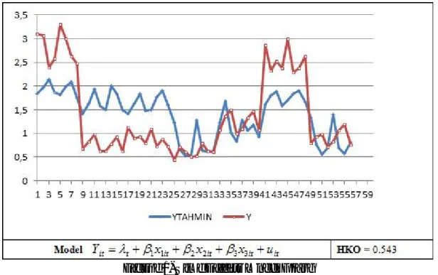
Figure 1. Graphs of individual effects model

The observed y and predicted values of y are shown in graph 1. Predicted value which is obtained from individual effects is close to observed y. Error mean square is 0.0286 for the individual effects model. F statistics equal to s 132.601 and it is greater than the critical value of F(6,46) =2,305. Consequently, null hypothesis is rejected so we decided

to there is a difference between units fixed effect model is significant

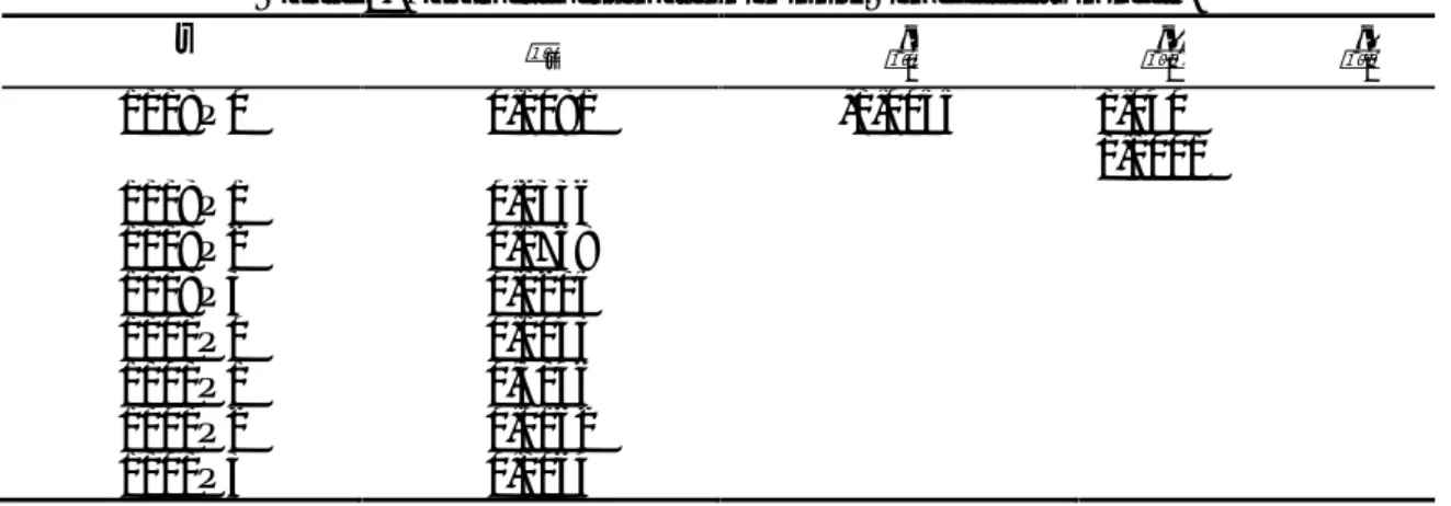
Table 2. Parameter estimation in only Time effects model.

t _{t }ˆ₁ 2 ˆ  ˆ₃ 2009Q1 1,2192 -0,1166 0,151 0,0112 2009Q2 1,3447 2009Q3 1,2879 2009Q4 1,0306 2010Q1 1,2154 2010Q2 1,4057 2010Q3 1,1273 2010Q4 1,0175

The estimate of t and ˆk estimators is shown in table 2. Critical level of F is greater than the F, null hypothesis is accepted and it means that there is no differences between time period over the units.

Figure 2. Time Effects Model Graph

In Fig.2 observations of Y and predicted values of y are given together. In time effect model, mean error square is 0.543 and it’s greater than the individual effect model. Random effect model is written as ,

1 1 2 2 3 3 1, ,7 1, ,8

it it it it

Y x  x  x  i  t   (22)

Table 3. Random effect models estimation

1

ˆ

 ˆ₂ ˆ₃

-0,099 0,1374 0,0248

Lagrange Multiple (LM)=145.744

Table 3. contain LM test statistics and the estimate of  . Critical level of _2 _{with 1}

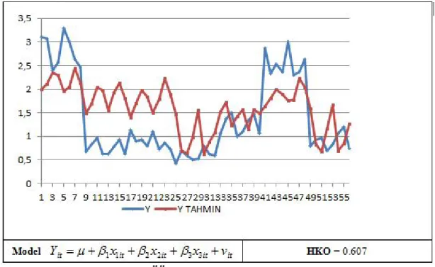
Random effects model is significant. Observations of Y and graphs of predicted values of Y shown in fig.3. For random effects model predicted values are not as good as prediction values of Y in fixed effect.

Figure 3. Random Effects Model Graphs 4. CONCLUSION

Panel data is common used method for economic data but it is rarely used for the meteorological data. This study aims at predicting average wind speed during the years 2009-2010 in the cities of Sinop, Samsun, Ordu, Kastamonu, Bartın, Zonguldak and Karabük of Blacksea Region by using wind speed, the average of maximum temperature, the average of minim temperature and the average of humidity. For individual effects model, MSE is 0,0286 and FE model is statistically significant. MSE is 0,543 in time effects model. In consequence of F test, one concludes that there are differences across the individual but not any differences over time period. The result

analyzing these data. Constant term which represented to individual is significant hence individuals are important to modelling for wind speed.

In this paper we showed that, panel data analysis can be used for meteorological data sets which include unit and time relation as an alternative method.

REFERENCES

Baltagi, H. Badi 2005. Econometric Analysis of Panel Data. John Wiley&Sons Ltd Greene, W.H. 2002, Econometric Analysis, Prentice Hall

Gujarati,D. Basic Econometrics .2004. The McGraw−Hill Companies Hsiao Cheng.2003. Analysis of Panel Data.Cambridge University Press

Matyas, L. , Sevestre . P., The Econometrics Of Panel Data : Advanced Studies In Theoretical And Applied Econometrics Volume 46, Fundamentals and Recent Developments in Theory and Practise, 2008. Springer

Sayyan H., 2000 Dinamik Panel Veri Modelleri Ve OECD Ülkeleri Para Talebi Uygulaması Doktora Tezi Marmara Üniversitesi Sosyal Bilimler Enstitüsü Ekonometri Anabilim Dalı

Tüzüntürk, S., 2005, İşlem Sıklığı Ve Hacmi İle Fiyat Volatilitesi İlişkisi : İMKB Örneği Yüksek Lisans Tezi Uludağ Ünver sitesi Sosyal Bilimler Enstitüsü Ekonometri Anabilim Dalı

Roy, N. 1997, Nonparametric and Semiparametric Analysis of Panel Data Models: An Application to Calorie-Income Relation for Rural South India. Doctor of Philosophy, Graduate Program in Economics, University of California.