Cumulant based identification approaches for nonminimum phase FIR systems

(1)

I576 IEEE TRANSACTIONS ON SIGNAL PROCESSING. VOL. 41, NO. 4 , APRIL 1993

Cumulant Based Identification Approaches for

Nonminimum Phase FIR Systems

Saleh A. Alshebeili, Member, IEEE, A . N. Venetsanopoulos, Fellow, IEEE, and A. Enis Cetin, Member, IEEE

Abstract-In this paper, recursive and least squares methods for identification of nonminimum phase linear time-invariant (NMP-LTI) FIR systems are developed. The methods utilize the second- and third-order cumulants of the output of the FIR system whose input is an independent, identically distributed (i.i.d.) non-Gaussian process. Since knowledge of the system order is of utmost importance to many system identification al- gorithms, new procedures for determining the order of an FIR system using only the output cumulants are also presented. To illustrate the effectiveness of our methods, various simulation examples are presented.

I. INTRODUCTION

N this paper, we introduce new parametric approaches

I

to the identification of nonminimum phase linear time- invariant (NMP-LTI) systems. The parametric model that we consider is an MA model described by

Y

y ( n ) =

C

h ( i ) x ( n - i) (1)

where y ( n ) is the output of an FIR system whose input is x ( n ) . The system input x ( n ) is assumed to be non- Gaussian, i.i.d., random process with E { x ( n ) } = 0, E { x ( n ) x ( n

+

7)) = & 6 ( 7 ) , and E { x ( n ) x ( n

+

~ ~ ) x ( n

+

T ~ ) } = & 6 ( ~ ~ , Q). This model is a special case of the general ARMA model; however, it has been widely stud- ied not only for its own interest but also due to the exis- tence of some methods which use MA estimation techniques to identify ARMA models [7].

Most of the standard system identification algorithms available in the literature estimate only a spectrally equiv- alent minimum phase system because these techniques exploit only the second-order statistics which suppress all phase information of the underlying process; thus they are incapable of identifying the nonminimum phase structure of the system. A recent approach to the identification problem of NMP-LTI systems is the use of polyspectra or higher order spectra. This approach exploits the fact that

i = O

Manuscript received March 26. 1991; revised May 26, 1992. This work was supported by NSERC, Canada, and TUBITAK. Turkey. Parts of this paper were presented at the IEEE 1991 International Conference on ASSP. Toronto. Canada. and at the 1991 International Conference on DSP, Flor- ence, Italy.

S. A . Alshebeili is with the Department of Electrical Engineering. King Saud University, Riyadh I142 I , Saudi Arabia.

A . N . Venetsanopoulos is with the Department of Electrical Engineer- ing, University of Toronto. Toronto. Canada M5S IA4.

A . E. Cetin is with the Department of Electrical and Electronics Engi-

neering, Bilkent University, Bilkent 06533, Turkey. IEEE Log Number 9206889.

the ( k

+

l)st-order spectrum ( k

>

1) which is the spec- trum of the (k

+

1)st-order cumulant sequence contains information regarding both the phase and magnitude of the Fourier transform of the system; and thus it has an advantage over procedures relying solely on the power spectrum in that perfect reconstruction is possible even when the system is nonminimum phase [lo].

Several methods utilizing cumulant statistics for the identification of NMP-LTI systems have been proposed in the literature (see, for example, [9]). Recently, Gian- nakis and Mendel [ 5 ] , and Tugnait [ 121 developed recursive and least squares identification methods by using the second-order statistics and a 1-D slice of the output cumulants. In this paper, we present new cumulant based identification methods by exploiting a much larger data set of output statistics. First, we propose a method that uses all samples of the second- and third-order cumulants to reconstruct the unknown system impulse response h ( n ) . Second, we develop cumulant based identification methods using the power spectrum and a 1-D slice of the bispectrum.

The methods presented in this paper require solution of a system of linear equations. Identification methods that exploit all the relevant statistics and use nonlinear opti- mization techniques are developed in the literature; see [ 3 ] , [9], and [ 141. Nonlinear solutions are computation- ally expensive and may converge to a local minimum. However, the estimates obtained via nonlinear solutions are generally better than the estimates obtained via linear solutions provided that the first are properly initialized. A good linear method can provide such an initialization that not only may lead to global convergence but may reduce the computational complexity as well.

An important problem in system identification is the determination of the system order. In this paper, this problem is also considered. New procedures for determining the order of an FIR system using only the output cumulants are proposed. In order to demonstrate the effectiveness of our methods, various simulation examples are presented.

11. A FUNDAMENTAL RELATIONSHIP In this section, we derive a relationship between the second- and third-order spectra. This relationship is of fundamental importance because it is the basis of our system identification algorithms.

(2)

ALSHEBEILI cf o l . : IDENTlFlCATION APPROACHES FOR FIR SYSTEMS 1577 Let us assume that we are given the second- and third-

order cumulants of the output sequence (in practice they can be estimated), then we can reconstruct the following

2-D sequence

Let us define the sequence g ( 7 , , Q ) such that

where

*

denotes convolution operation. Equation (3) is

the key equation for reconstructing h ( n ) from the second- and third-order statistics. In the frequency domain, (3)

becomes

(4)

where C2(w) and

C3(w1,

w 2 ) are the power spectrum and bispectrum, respectively. It is well known that the bi- spectrum is related to the system transfer function H ( w )

( 5 ) and the power spectrum is related to the system transfer function by

by

C 3 ( W I , w2) = P 3 H ( w l ) H ( W 2 ) H ( - W I - w2)

C 2 ( 0 ) = P * H ( w ) H ( - w ) . (6) By substituting ( 5 ) and (6) into (4), G ( w l , w2) can be writ-

ten in terms of the system transfer function as

(7)

where E =

p 3 / p 2 .

Bearing in mind (4) and taking the inverse Fourier transform of both sides of (7), we obtain the relationship

U

q

=

c

Eh(i)h(T2 - T~

+

i)c2(71 -

i )

₍₈₎ which relates the system response coefficients to the second- and third-order cumulants. Equation (8) is not new.

It has been first derived in [3] and [12]. In the next sec-

tion, we develop a new approach that exploits all the relevant statistics i n the solution of (8); and in Section IV,

we use (7) in the development of new approaches for the identification of NMP-LTI systems using slices of higher order spectra.

The basic equations used in [5] and [12] can be ob-

tained from (8). Giannakis and Mendel’s method utilizes the second-order statistics and the diagonal slice c 3 ( 7 , 7)

of third-order cumulants. By setting 71 = r2 = 7 in (8),

we get

i = 0

4 4

i

C

= 0 h ( i ) c , ( ~ - i, 7 -

i >

= i = O

C

6h2(i)c2(7 - i). (9)

If we multiply both sides of (9) by 1 / ~ , the resulting equation is called Giannakis and Mendel’s equation or simply GM-equation.

Tugnait’s method, on the other hand, utilizes the second-order statistics and the 1-D slice c 3 ( q , 7) of third-

order cumulants. By setting T~ = q and r2 = 71

+

q in (8), we obtain Tugnait’s equation (also called T-equation), that is,

4

i = O

C

h ( i ) c , ( q , i - 7) = Eh(O)h(q)C2(7) (10)

where we have used the fact that c3(i, i

+

q) = c 3 ( - i ,

q ) = c 3 ( q , -i). It is of interest to note that while both methods utilize a l - D slice of third-order cumulants, (9)

makes use of more correlation information than (10) does.

Methods based on simultaneous use of both (9) and (10)

are considered in [ 131.

111. RECONSTRUCTION FROM THE SECOND- A N D THIRD- ORDER CUMULANTS

A . Least Squares (LS) Method

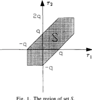
In this section, we develop least squares method for reconstructing the system impulse response coefficients ( h ( i ) } from the second- and third-order statistics of the output sequence y ( n ) . The method is based on using (8). Concatenating (8) for 71, r2 E S , where S is a region shown in Fig. 1 , we obtain the following system of linear equa- tions: where r = d = dl = d2 = d =

Mr

(1 1)

(h(1)

.

* * h ( q ) E Eh(1) * * Eh(q) Eh2(1)

& ( l ) h ( q ) * * Eh2(qf - (q2

+

5q

+

2 ) / 2 col-

-

c3(0, q ) ) , (c3(l, - q

+

1) * * c3(1, q )

.

* * c3(q. 0) *

.

* c3(q, q ) 0

. .

* 0) * *

and M is a matrix of size (5q2 + 4q

+

1) X (q2

+

5q

+

2)/2 whose entries are determined according to (8). The

least squares solution of this overdetermined system of equations is

r = ( M T M ) - ’ M T d . (12)

In solving (1 l ) , we assume without loss of generality that

the impulse response has been scaled so that h ( 0 ) = 1 . The unknown coefficients h (l), h (2), * * , h ( q ) can then

be determined as the first q elements of the vector r . This would be the end of the matter when there are no mea- surement noise and estimation errors. If this is not the case, we propose an alternative approach which exploits all the available information provided by the vector r .

(3)

1578 IEEE TRANSACTIONS ON SIGNAL PROCESSING, VOL. 41, NO. 4, APRIL 1993 and

h,(n) = k 2 z I ( n ) 0 I n I q

+

1 (17)

where k , and k2 are constants. By scaling the singular vec-

tors

zI

and u I so that

zI

(0) = u i (0) = 1, the unknown parameters E , h ( l ) ,

.

-

, h ( q ) can be determined from (16) and (17) in a straightforward manner. Alternatively, we could use the following expressions (which follow from (14) and ( 1 5)) to avoid division by a small value:

I

Fig. I . The region of set S

First, we form the matrix R from the vector r as follows:

. . .

(13)

It is clear from the structure of R that its rank is one. R can be written in the following form:

R =

h,hT

h ( n ) =

z I

(0) V ( 0 , O ) u l ( n ) 0 I n I q ₍₁₈₎ h,(n) = u l ( 0 ) V ( O , O ) z l ( n ) 0 5 n I q

+

1 . (19) It is relevant at this point to mention that theoretically only one singular value of R is nonzero. In practice, due to noise and estimation errors, there may be many nonzero singular values, but only a single dominant one. In fact, when the number of realizations approaches infinity, this dominance will be more pronounced.

Extension of the above described method to the fourth- order cumulant is provided in the Appendix.

B. Uniqueness of the LS Solution

The least squares method described in the previous section yields a unique (least squares) solution if the matrix

M

has full rank. In this section, we show that the matrix M is of full rank. Towards this objective, we first show that the unknown parameters { h

(i

)} and {eh ( i ) h ( 7 2 - 71

+

i)}, elements of the vector r , can be uniquely determined from (8) using a recursive algorithm. By setting T~

- r2 = -q in (8), we obtain -

where we have used h ( 0 ) = 1 . Similarly, by setting T~ = -4, we obtain

The unknown impulse response sequence h ( n ) can now

7 2 = -9

+

1, * * * , 0

be identified from the matrix R using one of the elegant techniques in numerical algebra; the singular value de-

Eh(72 + q) = c,(-q, 7 2 )

c2(-q)

(21)

composition (SVD). That is, R = Z V U T

(15) and where V is a diagonal matrix, the diagonal elements of which are the singular values of R . The columns of the singular vectors of R , and the columns of the second unitary matrix U , that is, u i , u2, , u I + q , are the right

singular vectors of

R .

Since R is of rank one, it follows that there is only one nonzero singular value, whose corresponding singular vectors determine the impulse response. From the properties of the SVD, it can be shown

~ 3 ( - q , 72) - - c3(-q7 72)

ec2(-q) c3(-q, -4) h(72

+

4) =

unitary matrix Z , that is, ZI, z2,

-

.

, z2 + q , are the left

72 = -4

+

1, ' * , 0. (22)

*

The unknown Parameters (Eh(iIh(72

-

7 2 + i ) > can be obtained from (8) as follows. First, we compute Eh2 ( q ) by

7~ = 72 = 2q, that is,

.

-that [ 81

(4)

ALSHEBElLl (’I U / . : IDENTIFICATION APPROACHES FOR FIR SYSTEMS

Then, we use the following recursive formulas:

F o r n = 1 to Lq/2) fh(n)h(7*

+

4 ) 71 = -4

+

n and r2 = -q

+

n ,

-

C . Robustness to Additive Noise

In practical applications, the received signal is usually a noise corrupted version of the original one. In this section, we consider the signal model

where d ( n ) is the received signal, and w ( n ) is an additive Gaussian noise.

For Gaussian processes only, cumulants of order greater than two are identically zero. This property can be exploited in estimating the third-order cumulants of noisy observations. Under the assumption that w ( n ) is inde- pendent of y ( n ) , the third-order cumulants of d ( n ) are equal to the third-order cumulants of y ( n ) . Symbolically,

1.579

This indicates that c3, ( T ~ , 7 2 ) are not affected by additive

Gaussian noise. The second-order cumulants, on the other hand, appear to be affected by presence of noise, because

If the second-order cumulants of the additive noise are nonzero only for lags in the range 171

<

i j where

(q/2) - 1 if q is even

( q - 1)/2 if q is odd (29)

the recursive method developed in the previous section for reconstructing the unknown parameters { h

(i)}

and { ~ h ( i ) h ( ~ ~ - 71

+

i)} from the second- and third-order cumulants will not be affected by presence of noise since it uses samples of c2,,(7) for which

4 <

171 5 q. Conse- quently, uniqueness and consistency of the LS solution will remain unaffected if the rows of the matrix M which contain the samples of c2,, (7) are removed.

IV. RECONSTRUCTION FROM THE POWER SPECTRUM A N D A 1-D SLICE OF THE BISPECTRUM Another possible approach to reconstructing h (n) from the output data { y ( n ) } is to use slices of higher order spectra [ l ] , [2]. In this section, we present recursive and least squares methods for reconstructing h ( n ) from the power spectrum and a 1-D slice of the bispectrum. The methods utilize the 1-D slice corresponding to wI = w 2 .

By substituting wI = w2 = w in (7), the following relationship results:

Multiplying both sides of (30) by C2(2w)H(2w), we ob-

tain

(3 1)

H(2w)

c,

( U , w ) = EH2 (a)

c,

(2w). In the time domain, (31) takes the form

2u 20

- I

r

C

= o h l ( i ) c ’ ( 7 - i ) = r = O

c

th2(i)s’(7 - i) (32) where

Equation (32) is the basis for our recursive and least squares methods.

(5)

n -

i)

term 2 = ~ ~ : ~ , , ‘ h , ( i ) s ’ ( - 2 q

+

n - i ) h,(n) = (term 1 - term 2 ) / c ’ ( - 2 q ) h ( n ) = ( h 2 ( n ) - C : Z : h ( i ) h ( n - i ) ) / 2 e‘ ( - 2 4 (33) end E = -

where we have used h ( 0 ) = 1 . Once we obtain E , we can proceed to compute the first parameter h (1) by setting 7

= -2q

+

1 . By doing so, we obtain

The above algorithm is well conditioned in the sense that all divisions are done through c2 (-4) and c‘ ( - 2 q )

which are nonzero for an MA ( q ) model.

c ’ ( - 2 q

+

1 ) c ’ ( - 2 q

+

1)

.

(34) B. Least Squares (LS) Method -

- h , ( l ) =

ec,(-q) c’ ( - 2 4

The recursive method presented in the previous section Since we know that introduces propagating errors when the initial estimates of h (n) are inaccurate; in addition, it does not smooth out lems, we develop in this section a least squares solution for (32). Generally, ( 3 2 ) can be written in a matrix form 4

0

. .

-

Similarly, by setting 7 = -2q

+

2 , we can compute h 2 ( 2 )

from which we can get h ( 2 ) . In general, the unknown

parameters of the MA model described by (1) can be re-

The least squares solution of this overdetermined system of equations is

(6)

1581

ALSHEBEILI et al.: IDENTIFICATION APPROACHES FOR FIR SYSTEMS

Once we obtain 6 , the sequence h ( n ) can be recovered from the first q elements of 6 . That is, h ( n

+

1) = b ( n )

for 0 5 n 5 q - 1; or it can be recovered from the laser 2q

+

1 elements of b using recursive and nonrecursive methods. If we define z to be as follows:

and q = Eh(O)h(q). Combining (37) and (43) yields = ( 0 6 ? + I ) x l

D'

0,2q + 1 ) x (2q + I )

)

(;)

(45)

where

z = (1 b ( q

+

l)/b(q) * b(3q>/6(q))T (40) matrix whose entries are

OM - A' identically zeros. then

h ( n ) = 5

-'

[ 5

[z

( n ) ]

1;

z

(0) = 1 (41) The coefficient matrix of the above system of linear equations is a full rank matrix, since the elements: q , { h ( n ) } , and {eh2(n)) of the unknown vector of (45) can be recursively determined from (10) and (32) as shown below.

T = q in (lo), respectively: or recursively

(46) First, we compute 7 and h ( q ) by setting 7 = - 4 and

(47) c3(q, 4 ) c2 ( 4 ) vc2 ( 4 ) h ( q ) = ~ c3(0, 4 ) '

r = -

(42)

may lead to numerically unstable solution (very high magnitude of the estimated coefficients) if Ib(q)l ( = It/)

I1 - 1

h ( n ) =

(

z(n> -

.C

h ( i ) h ( n - i ) 2 1 5 n 5 q r = l

where h ( 0 ) = 1. Let us, however, note that using (40)

is to be severely underestimated.

Once q is determined, the unknown MA coefficients { h ( n ) } can be recovered from (10) as follows [12]:

F o r n = 1 to Lq/2J

n - , C. Modijied LS Solution

The uniqueness of the LS solution of (39) is guaranteed

h ( n ) = ( q c 2 ( q - n ) -

C

h ( i ) c , ( i + q

provided that the matrix

D

has full rank. However, it is , = n

s:,.(7 - i)} (51)

where we have used (26)-(28). To obtain consistent parameter estimation, (51) should not be used for 0 I 7 5

2q if w ( n ) is a white Gaussian noise, and for -2q 5 7 5

2q

+

2q if w ( n ) is a colored Gaussian noise with

Similarly, (52) should not be used for 7 = 0 if w ( n ) is a white Gaussian noise, and for 171 I Zj if w ( n ) is a colored Gaussian noise whose second-order cumulant is given by (53).

The recursive method developed in Section IV-A utilizes (32) for lags in the range -2q 5 7 I -9. And the recursive method developed in Section IV-C utilizes (10) for lags in the range 171

>

q,

and (32) for lags in the range -2q I 7 I -q and 3q 5 7 5 4 q . Therefore, they are

not affected by presence of a Gaussian noise with a sec- ond-order cumulant as in (53). As a consequence, the LS solution of ( 4 5 ) will also remain unaffected if the rows of B that contain the samples of ~ ~ ~are removed. In con- ( 7 )

trary, the LS solution of (37) is affected by presence of a colored Gaussian noise. It can only handle a white Gaussian noise, and that is by removing 2q

+

1 rows of the matrix D which contain the sample c2,,,(0).

V. PROPERTIES OF THE NEW METHODS

In this section, we present the properties of the NMP

system reconstruction methods described in Sections I11 and IV.

1 ) There is a close relationship between the LS solution of Sections I11 and IV. Specifically the matrix R can be decomposed into two matrices as shown below:

* . .

. . .

( 5 4 ) ( 5 5 )

(8)

ALSHEBEILI e / U / . : IDENTIFICATION APPROACHES FOR FIR SYSTEMS By projecting the elements of the matrix R2 onto its diagonal, we can form the following vector:

U = ( E 2 ~ h ( l ) e ( h 2 ( 1 )

+

.

* * _{2 ~ h ( q} - l ) h ( q ) Examining ( 5 6 ) , it is clear that

n v ( n ) =

C

~ ~ ( i ,

n - i) = E ( h ( n )

*

h ( n ) ) = i = O where v ( 0 ) = R2(0, 0) = E , and u ( 2 q ) = R 2 ( q , q) = Eh2 ( 4 ) .

2) Instead of applying the SVD to the matrix R given by (13), we could have applied it to the matrix R2 given by (55). R2 has rank one and can always be written as

R2 = h,ha

In theory, n ) } , { k @ ) / h , ( O ) ) , and { h , ( n ) ) are identical. In practice, due to noise and estimation errors, they are different; and as such, we have three candidates to the unknown coefficients ( h ( n ) } . They are

h'"(n) = R ( 0 , n )

h'2'(n) = h,(n)

h'3'(n) = h , ( n ) / h , ( O ) 0 5 n 5 q. (59)

To choose one candidate out of the others, we select h(')(i

= 1, 2, 3 ) which minimizes the squared differences between the observed cumulants and the cumulants of the proposed model.

3) It is possible to remove the redundancy present in the unknown parameters of (1 1 ) and (37). Consider, for

instance, the LS method of Section 111. Multiplying both

sides of (7) by H ( w ,

+

w 2 ) and taking the inverse Fourier transform, we obtain

9

i = O h ( i ) g ( T I - i, 7 2 - i) = ~ h ( ~ I ) h ( 7 2 ) (60)

where g(71, 7 2 ) = 5-l[G(wl, w 2 ) ] . The right-hand side of (60) is nonzero only in the region 0

cc

71, 7 2 5 q. If 71, T~

<

0 or 71, 7 2

>

q , (60) reduces to

4

h ( i ) g ( 7 , - i , 7 2

-

i) = -g(71, T ~ ) (61)

where we have used h ( 0 ) = 1. The above equation can be written in a matrix form and then be solved for the unknown parameters h ( l ) , h ( 2 ) , * *

.

, h ( q ) . Let

us,

however, note that the solution so obtained is affected by presence of additive Gaussian noise since it uses all sam-

i = I

1583

ples of the second-order cumulants. In addition, H ( z ) should not have zero(s) on the unit circle.

4) The RC and LS methods in Section IV can be ex-

tended in a straightforward manner to the fourth-order spectra. If C4(w, w , w) is the l-D slice of the fourth-order spectrum, G(w) will be related in this case to the system transfer function H ( w ) by

where G(w) = C4(w, w, w)/C2(3w), and C2(3w) is the Fourier transform of the sequence

c2 (7/3) if

7

= integer otherwise. (63) 3 39

L

s'(7) =

In the time domain, (62) takes the form

3q i = O

C

h , ( i ) c ' ( 7 - i) = i - 0

c

e h 2 ( i ) s ' ( 7 -

i)

(64)

where h l ( n ) = 5 - I [H(3w)] h2 ( n ) = 5 - I [ H 3 (a)] c'(7) = 5

-'

[C4(0, 0 , a)].

Equation (64) resembles ( 3 2 ) . Therefore, it can be solved in a procedure similar to that in Section IV using recursive

and least squares methods. Extension of (IO) to the fourth- order cumulants is straightforward and is given by [ 121

9

h ( i ) c , ( q , q, i

-

7 ) +'c2(7). (65)

I = o

VI. SYSTEM ORDER DETERMINATION

In this section, we address the problem of system order determination using cumulant statistics. Knowledge of the system order is of utmost importance to many system identification algorithms. In [6], two methods were sug-

gested for determining the order of an FIR system using

exp (-c2/2a2) dc = 1 - eo (66)

for a given probability of error eo, where a 2 is the variance of the random variable c 3 ( q

+

1, 0) and t, is a threshold. Obviously, the first method is impractical, while the second is dependent on statistics of a single random variable

-

37 s-,.

(9)

IEEE TRANSACTIONS ON SIGNAL PROCESSING, VOL. 41, NO. 4 , APRIL 1993 I584

In the following, we propose a new procedure for determining the order of an FIR system using the second- and third-order cumulants of the output sequence. The method presented depends neither on visual inspection nor on statistical tests. In addition, it utilizes a much larger data set of output statistics than does (66).

It is well known that the third-order cumulants of an FIR system are identically zero for lags outside the region defined by -q I T ~ , r2 I q (see Fig. 2 for an exact definition). From (lo), the unknown impulse response h ( n ) of an FIR system is related to the second-order cumulants c2 (7) and the 1-D slice c3 (4, 7 2 ) of the third-order cumulants ~ ~ ( 7 1 , 72) by

4

h ( i ) c 3 ( i - 7, q ) = v c 2 ( 7 ) . (67) i = O

Equation (67) can be rewritten in a matrix form as (68) d ‘ = D ’ b ’

where d ’ , D ‘ , and b‘ are defined as in (43). cumulants can be computed as follows [9]:

If

p3

= 1 and q is the true system order, the third-order

4

r = O

C;(71, r 2 , q) =

,E

h ( i ) h ( i

+ ~ ~ ) h ( i

+

72) (69) where C ; ( T ~ , r2; q) denotes the third-order cumulants

computed by using the estimated impulse response coefficients h(1) * h ( q ) obtained from solving (68).

Let us now define the function e ( T ~ , r2; q’) as follows:

e(71, 7 2 ; 4’) = c3(71, 7 2 ) - c;(71, 7 2 ; 4’). (70)

Theoretically, e ( T 1 , 7 2 ; q’) should be zero when q’ = q. The system order determination algorithm that we propose is based on the following steps:

1) From the given data, compute the second-order cu- mulants c2 (7; p ) in the region defined by 0 I 7 I p where

P

>

4.

2) From the given data, compute the third-order cu- mulants c3(71, 7 2 ; p ) in the region bounded by the lines 7 l = 0, and 71 = T ~ ; 0 I T ~ , r2 I p .

3) From (68), compute the unknown coefficients h(1)

h ( q ’ ) assuming the order of the system is 4’; 1 I q’ 4) Find the value of q’ which minimizes the following

I p . performance measure: D 71 a’ 7 1 r, 71 1 I q’ I p . (71)

Note that C ; ( T ~ , r2; q’) = 0 for T~

>

q’. Theoretically,

t

T 2

a /

F i g . 2 . The region of support of third-order cumulant of an M A ( y )

s y s t e m .

E ( q ’ , p ) = 0 when q‘ = q. In practice, due to noise and estimation errors, E ( q , p ) # 0 but of minimum value. In deriving the above algorithm, we have used

p3

= h ( 0 ) = 1. If h ( 0 ) # 1 (or

p2

# l ) , the sequences c3(71, 72) and

C ; ( T ~ , 7 2 ) should be properly scaled to ensure that e ( 7 1 ,

r2; q ) = 0 when C ~ ( T ~ , T ~ ) is the true cumulant sequence.

One possible approach to doing this is to normalize c3 ( T ~ , T ~ ) and c; ( T ~ , 72) by their zero samples at the origin. The samples c 3 ( 0 , 0) and c i ( 0 , 0) should not in this case be equal to zero.

The above described algorithm is affected by presence of additive Gaussian noise since it utilizes the second- order cumulants. However, if the second-order cumulants of the additive noise are nonzero only for lags in the range (71 5 Zj, the effect of the noise can be eliminated by de- leting the rows of the matrix D corresponding to 171 I

9.

The matrix D so modified remains of full rank [ 121. Instead of computing c; ( T ~ , r2; q ) using the second- and

third cumulants, we could have computed it using the third-order cumulants only. In [4], a relationship between the system impulse response h ( n ) and the 1-D slice c 3 ( q , 72) has been derived. This relationship is given by

By substituting (72) into (69), we obtain

(73) Equation (73) is useful when the output data is contami- nated by additive, colored Gaussian noise with unknown statistics.

It is relevant at this point to mention that the system order determination algorithm described above can be applied to AR(q)-type processes, as well. If { y ( n ) ) corre- sponds to an AR(q) model of order q , then its inverse statistics correspond to an MA ( q ) process. To see this, let

(10)

ALSHEBEILI PI U / . : IDENTIFICATION APPROACHES FOR FIR SYSTEMS 15x5

B(w,, w 2 ) denote the bispectrum of an AR(q) process described by

Then

where H ( w l , w 2 ) is the bispectrum of h ( n ) . The inverse

bispectrum of y ( n ) is the bispectrum of h ( n ) scaled by y = 1 / & . That is,

By computing the finite extent third-order cumulants of h ( n ) which is the inverse Fourier transform of H ( w l , w z ) ,

the algorithm of this section can be applied to determining the unknown order q. It is relevant at this point to notice that the third-order cumulants of h ( n ) can also be com- puted from the third-order cumulants of y ( n ) using a set of linear equations [ 1 1 ] :

(77)

where (77) is derived by computing the inverse Fourier transform of both sides of the equation B ( w l , w 2 ) H ( a I ,

w2) =

&.

Equation (77) can be written in a matrix form and then solved for the unknown cumulant samples of h ( n ) for lags in the region 0 I r l , r2 5 q and r , 5 r2.

VII. SIMULATION EXAMPLES A . System IdentiJcation

generated by the signal model [ 121 :

In this simulation example, the available data { d ( n ) } is

+

3.02x(n - 3)

- 1 . 4 3 5 . ~ ( ~ - 4)

+

0 . 4 9 ~ ( n - 5 ) + ~ ( n )

where the input signal x ( n ) is zero-mean exponentially distributed i.i.d. noise generated by the GGEXN subroutine of the IMSL library with

f13

= 1 . The zeros of the unknown system transfer function H ( z ) are located at - 2 ,

0.7 j0.7, and 0.25 +_ j0.433. The signal w ( n ) is an additive noise which is zero-mean white Gaussian process generated by the GGNML subroutine of the IMSL library.

Three different lengths of output data was used in this study: N = 1024, 2048, and 4096. The impulse response coefficients of the unknown system were computed for 100 output realizations at signal-to-noise ratio (SNR) = 03

(noise-free case) where SNR = E{ y

* ( n )

]

/ E

{ w ( n )

1.

Besides the noise-free case, the impulse response coefficients were also computed for N = 4096 at SNR = 100 and I O . The second- and third-order cumulant sequences were computed using the indirect estimation method described in [ 101. For each run, we also calculated the mean squared error (MSE) defined as

where h ( n ) and h,(n) are the true and reconstructed impulse responses, respectively. Tables 1-111 show the mean values and standard deviations of the various parameters when the LS solutions of Section 111-A (LS-I), Section IV-C (LS-U), and Tugnait’s method [I31 (LS-T) are em- ployed. For the noisy cases, rows of the coefficient matrix that contain the sample c Z d ( 0 ) are removed. Based on the results obtained, we observe that: i) LS-I1 has lower MSE than LS-T, and ii) the estimates obtained via LS-I are generally better (in terms of variance and MSE) than the estimates obtained via LS-I1 and LS-T. This is, however, expected since the data set of output statistics exploited by LS-I is much larger than the data set of output statistics exploited by LS-I1 or LS-T; for example, LS-I utilizes all slices of third-order cumulant whereas LS-T utilizes only two slices of it.

B. Order Determinution

In this section, we present an example demonstrating the use of the order determination algorithm described in Section VI. Seven independent realizations were gener- ated using the signal model [6]:

d ( n ) = X ( H )

+

0 . 9 , ~ ( ~ - 1)

+

0 . 3 8 5 ~ ( n - 2)

where x ( n ) and w ( n ) are defined as in (78). Table IV shows the value of E ( q ’ , p ) computed at q’ = 1, 2,

. . .

, 5 ; with p = 5 , SNR = 10, and N = 1024. Based on the results obtained, it is clear that E ( @ , p ) attains its mini- mum when q’ = q = 3.

In order to illustrate the effectiveness of our algorithm, 100 Monte Carlo runs for determining the order of the system described in (80) were performed at SNR = 10

and N = 512, 1024, 2048, and 4096. Table V shows the number of successful selections of the MA order when the algorithm of Section VI was implemented using (69) and

(73). For comparison, the Giannakis-Mendel’s algorithm [6] was also tested using the same data. The parameter E”

(11)

15x6 IEEE TRANSACTIONS ON SIGNAL PROCESSING, VOL. 41, NO. 4 . APRIL 1993 TABLE I

T H E RECONSTRUCI-ED IMPULSE RESPONSE OF T H E S I M U L A T I O N E X A M P L E U S I N G LS-I A N D 100 MON.I t, C A R L O RLss ( p = MEAN. U = S TA ND A R D

DEVIA.TION, A N D MSE = M E A N S Q I J A R B I ) ERROR)

SNR = m N = 4096 N = 1024 N = 2048 True Value P U P U 0.100 -0.0196 0.2407 -0.1294 0.2284 - 1.870 -0.7005 0.4349 -0.9627 0.4099 3.020 1.3730 0.6648 1.8499 0.5575 0.490 0.2182 0.1137 0.2950 0. I043 - 1.435 -0.7510 0.3224 -0.9748 0.2430 N = 4096 P U -0.1251 0.2259 - 1.2402 0.3934 2.2705 0.4670 0.3455 0.0820 -1.1461 0.1641 SNR = 100 SNR = 10 P U P U -0.1025 0.1688 -0.0873 0.1973 -0.8926 0.4207 -0.8150 0.4255 1.2265 0.5742 1.0992 0.5530 0.1137 0.0994 0.0943 0.0930 0.4930 0.3096 -0.4281 0.2741

MSE 0.3431 0.2246 0. I940 0. I677 0.0984 0.1004 0.3690 0.2159 0.4151 0.2168

TABLE I1

T H F RECONSrRLlCrED IMPULSE RFSPONSF O F T H F SIMULATION E X A M P L E U T I N G LS-11 A N D 100 MOhTF CAR1 0 R U N T ( p = MFAN. U = S I 4 h D A R D DEVIATlOh, A N D MSE 1 MFAN S Q l J A R F D ERROR)

SNR = m N = 4096 N = 1024 True Value P U 0.100 0.2839 0.7190 3.020 1.7987 0.6245 0.490 0.0031 0.4167 -1.870 -1.3817 0.7001 - 1.435 -0.4836 0.5523 N = 2048 N = 4096 SNR = 100 SNR = 10 P U 0.2453 0.6807 2.1656 0.5477 0.0999 0.3813 - I 3 7 7 0.5620 -0.7231 0.5478 P U 0.2578 0.621 1 2.5424 0.3890 0.2215 0.3487 - 1.7870 0.4328 -0.9542 0 4992 P U 1.2010 0.7356 1.3117 0.0395 0.1908 0.2047 -0.5068 0.9958 -0.5989 0.5070 P U I . I615 0.7285 1.2876 0.9961 0.1780 0.2238 -0.5222 0.9731 -0.5564 0.5083 MSE 0.2991 0.2143 0.1883 0.1682 0.1034 0.1163 0.6066 0.4086 0.6005 0.3785 TABLE I11

THE RECONSTRUCTED IMPULSE RESPONSE OF T H ~ S I M U L A T I O N E X A M P L ~ USING LS-T A N D 100 M O N I I C A R L O RUNS ( p = M E A N , U = STANDARL) D E V I A ~ - I O N , A N D MSE = MEAN S Q U A R ~ D ERROR)

_ _ _ _ _ _ _ _ _ _ _ ~ SNR = CO N = 4096 N = 1024 N = 2048 N = 4096 SNR = 100 SNR = 10 True Value P U I* U P U P U P U 0.100 -0.2909 0.5064 -0.1873 0.5773 0.0027 0.5502 0.6468 0.6362 0.5328 0.5381 3.020 0.8711 0.6721 1.2669 0.7381 1.7313 0.6618 0.8240 1.0982 0.7267 1.3145 0.490 0.0342 0.2639 0.1012 0.3018 0.1437 0.2724 0.2223 0.2169 0.2127 0.1845 MSE 0.6095 0.3519 0.4681 0.3351 0.2956 0.2823 0.7107 0.4646 0.7569 0.4912 -1.870 -0.5784 0.6101 -0.8704 0.6552 -1.2176 0.6145 -0.3376 0.9576 -0.3988 1.0141 -1.435 -0.1518 0.5276 -0.2877 0.6739 -0.4393 0.5687 -0.491 I 0.5839 -0.431 I 0.5603 TABLE IV

SYSTEM ORDER DETERhllNATlON USING SEVEN INDEPENDENT REALIZATIONS WITH p = 5. SNR = 10. A N D N = 1024

E ( 4 ' . p )

TABLE V

P E R b O R M A N C t E V A L U A rlON O b SYSThM O R D E R DETFRMINATION ALGORITHMS W I T H P = 5 , SNR = 10. A N D 100 MONTE CARLO RUNS 4' Run-I Run-2 Run-3 Run-4 Run-5 Run-6 Run-7 Number of Successful Selections

1 1.4200 1.0365 1.5786 1.6723 1.6873 2.7133 1.9147 2 2.7602 1.6311 2.7367 3.9544 3.0917 4.3189 3.2453 3 0.3767 0.3671 0.1238 0.3711 0.1375 0.5422 0.3347 4 2.2084 1.5434 2.8321 1.0652 2.8356 2.3786 3.1369 5 2.3805 2.8165 1.5221 1.9823 0.3146 3.8384 5.2588 Approach N = 512 N = 1024 N = 2048 N = 4096 Eq. (69) 83 85 96 100 Eq. (73) 84 91 93 99 161 I I 30 52 74

(12)

In this paper, new methods for the identification of non- Gaussian white-noise-driven NMP-LTI FIR systems are proposed. Recent developments on NMP-LTI FIR system identification include works by Giannakis and Mendel [5], and Tugnait [12], [I31 who considered FIR parameter estimation using the second- and one-dimensional (1-D) slices of output cumulants. In this paper, we show how to solve this problem using the second-order and all samples of third-order cumulants in an appropriate domain of support. Identification methods using the second-order cumulants and the diagonal slice of bispectrum are also developed. It is shown that the methods presented yield consistent parameter estimation in a class of colored

APPENDIX

The least squares method presented in Section 111-A can be extended to the fourth-order cumulant. The function

G(wl, 0 2 , w 3 ) can be expressed in terms of the system transfer function as follows:

c4(w1, w 2 ? w 3 ) G(wi, ~ 2~, 3 = ) C 2 ( W I + U2

+

w3) H(w1

+

U2 + w3) E H ( W 1 ) H(a2) H ( W 3 ) (82) - -

where E =

p4/&

and C 4 ( ~ 1 , w 2 , w 3 ) is the trispectrum of

(h,

WO h ( l ) r l

.

* * h ( q ) r J T (84)

where

ho = h ( 2 ) * h ( q ) ) ,

r, = (Eh2(i) Eh(i)h(i

+

I ) E h ( i ) h ( q )

eh2(i

+

1) ch(i

+

l)h(q)

-

* Eh2(q)),

h ( 0 ) = 1 and i = 0, 1, 2,

-

* , 4.

Once the vector r is determined, the matrix R is formed as follows:

1

Eh(1) E h ( l ) h ( l )

. . .

& ( l ) h ( q ) Eh(1)h2(1) dZ2(1)h(q) * * & ( l ) h 2 ( q )

R =

. .

\

:

. .

The matrix R has rank one, and can be written as Gaussian noise. Both recursive closed form and batch least

squares versions of the parameter estimators are presented. Extension of these methods to the fourth-order cumulants is also addressed.

A relevant problem in parametric modeling of higher order statistics is the determination of system order. In this paper, two new methods for determining the order of an FIR system using only output cumulants are also pre-

sented. The first method utilizes the second- and third- * * h ( l ) h ( q )

.

* * h 2 ( q ) ) . (86)

order cumulants, whereas the second method utilizes the

third-order cumulants only. It is shown by computer sim- The vectors hl and i can be determined from R using the ulation that our system order determination algorithms SVD.

outperform the existing cumulant based algorithms [6]. A matrix

R

can also be formed from the elements of the (1 h(1)

. .

* h ( q ) h2(1)

R = h 1 3 =

(13)

1588 IEEE TRANSACTIONS ON SIGNAL PROCESSING, VOL. 41, NO. 4 , APRIL 1993 [ I I] M. Rangoussi and G B Giannakis. “On the use of second- and higher

order inverse statistics,” in Proc Workshop Higher Order Spectral

Analysis, Vail, CO, pp 7-12, June 1989

[I21 J K Tugnait, “Approaches to FIR system identification with noisy data using higher order Statistics,” IEEE Trans Acoust., Speech, Signal Processing, vol 38, no. 7, pp 1307-1317, 1990.

[ 131 J K Tugnait. “New results on FIR system identification using higher order statistics,” in Proc Fifth ASSP Workshop Spectrum Estimation

Modeling, Rochester, NY. Oct. 1990, pp. 212-216; also in IEEE Trans Signal Processing, vol 39, no. 10, pp 2216-2221, 1991 [14] J K Tugnait, “Identification of linear stochastic systems via second-

and fourth-order cumulant matching.” IEEE Trans. Inform Theon’, vol 33, no 3. pp 393-407, 1987 vector i as follows: h2 ( 4 ) (87) h r

1.

1 h ( l ) h ( 2 )

.

* * R = ( h ( 1 )

:

h2(1) h ( l ) h ( 2 )

.

* * h ( l ) h ( q ) h ( q ) h ( q ) h ( l ) h ( q ) h ( 2 ) * * *

By applying the SVD to the matrix R , we find

( 1 h(1) * * h(q)). (88) Saleh A. Alshebeili (S’89-M’91) received the Ph D. degree from the Uni- He is currently with King Saud University, versity of Toronto in 1991

Saudi Arabia

R = h2h3 =

(+)

h (4)

Therefore, by using the fourth-order cumulant, four can- didates to the unknown system impulse response { h ( n ) } are obtained. They are: { h o ( n ) } , { h , ( n ) / h l (O)}, { h 2 ( n ) } ,

and { h , ( n ) } . With the exact knowledge of second- and

fourth-order cumulant samples, all the candidates are identical. The uniqueness of the (least squares) solution is guaranteed, since the coefficient matrix of (83) is of full

rank. This follows from the fact that the unknown parameters { h ( n ) } and ( ~ h ( i ) h ( 7 ~ - T~

+

i ) h ( T 2 - 71

+

i)} can be uniquely determined from (83) using procedures

analogous to those of the third-order cumulant described in Section 111-C.

Anastasios N. Venetsanopoulos (S’66-M’69- SM’79-F’88) received the B.S. degree from the National Technical University of Athens (NTU), Greece, i n 1965, and the M S . , M Phil , and Ph.D. degrees i n electrical engineering, all from Yale University. in 1966, 1968, and 1969, respectively.

He joined the University of Toronto, Canada, in September 1968, where he is now Professor in the Department of Electrical Engineering. He also served as Chairman of the Communications Group (1974 to 1978 and 1981 to 1986). and as Associate Chairman of the De- partment o f Electrical Engineering (1978 to 1979) He was on research REFERENCES

S . A. Alshebeili and A. E. Cetin, “A phase reconstruction algorithm

from bispectrum,” IEEE Trans. Geosci. Remote Sensing, vol. 28, no. 2, pp. 166-170. 1990.

A. E. Cetin, “Algorithm for signal reconstruction from bispectrum,” in Proc. 14th Biennial Symp. Commun. Signal Processing. Kingston, Ontario, Canada, May 1988, pp. D.2.5-8.

B. Friedlander and B. Porat, “Asymptotically optimal estimation of MA and ARMA parameters of non-Gaussian processes from higher order moments,” IEEE Trans. Automat. C o n f r . , vol. 3 5 , no. I , pp. 27-35, 1990.

G. B. Giannakis, “Cumulants: A powerful tool in signal process- ing,” Proc. IEEE, vol. 75, no. 9 , pp. 1333-1334, 1987.

G. B. Giannakis and J. M. Mendel, “Identification of nonminimum phase systems using higher order statistics,” IEEE Trans. Acoust.,

Speech, Signal Processing, vol. 37, no. 3 , pp. 360-377, 1989.

G. B. Giannakis and J . M. Mendel, “Cumulant-based order deter- mination of non-Gaussian ARMA models,” IEEE Trans. Acoust.,

Speech, Signal Processing, vol. 38, no. 8. pp. 141 1-1423. 1990. G . B. Giannakis and A. Swami, “On estimating noncausal non- minimum phase ARMA models of non-Gaussian processes,” IEEE

Trans. Acoust., Speech, Signal Processing. vol. 38. no. 3. pp. 478-

495. 1990.

G. H. Golub and C. F. Van Loan, Matri.r Computution. Baltimore, MD: Johns Hopkins University Press, 1983.

J. M. Mendel, “Tutorial on higher-order statistics (spectra) in signal processing and system theory: Theoretical results and some applica- tions,” Proc. IEEE, vol. 79, no. 3, pp. 278-305, 1991.

C. L. Nikias and M. R. Raghuveer, “Bispectrum estimation: A dig- ital signal processing framework,” Proc. IEEE, vol. 75, no. 7, pp. 869-891, 1987.

ieave at the Swiss Federalinstitute-of Technology, the University of Flor- ence, the Federal University of Rio de Janeiro, the National Technical Uni- versity of Athens, and the Imperial College of Science and Technology, and was Adjunct Professor at Concordia University. He served as Lecturer of numerous short courses to industry and continuing education programs; he is a contributor to eleven books and has published over 300 papers in digital signal and image processing, and digital communications; he also served as consultant to several organizations. and as Editor of the Canadian

Electrical Enginwring Journal (1981 to 1983).

Dr. Venetsanopoulos is a member of the New York Academy of Sci- ences, Sigma Xi, the lntemational Society for Optical Engineering, and the Technical Chamber of Greece; he is a Registered Professional Engineer in Ontario and Greece, a Fellow of the Engineering Institute of Canada, and a Fellow o f the Institute of Electrical and Electronics Engineers for con- tributions to digital signal and image processing.

A. Enis Cetin (S’85-’87) received the B.Sc. degree in electrical engineering from the Middle East Technical University, Ankara, Turkey, in 1984, and the M.S.E. and Ph.D. degrees in systems engineering from the Moore School of Electrical En- gineering, University of Pennsylvania, in 1986 and 1987, respectively.

From September 1987 to July 1989 he was As- sistant Professor of Electrical Engineering at the University of Toronto. During the summers of 1988 and 1991 he was a consultant and a resident visitor, respectively. at Bellcore, Morristown, NJ. He is presently Asso- ciate Professor of Electrical and Electronics Engineering at Bilkent Uni- versity, Ankara, Turkey.