Sosyal Ekonomik Araştırmalar Dergisi (The Journal of Social Economic Research) ISSN: 2148 – 3043 / Nisan 2015 / Yıl: 15 / Sayı: 29
TÜRKİYE’DE ENFLASYON HEDEFLEMESİ: VAR
ANALİZİ
Ceyhun Can ÖZCAN* Uğur ADIGÜZEL**
ÖZET
Enflsyon, 20 yüzyılın ikinci yarısından bu yana tüm ekonomilerin temel problemlerinden birini oluşturmaktadır. 90‟lı yılların başında bazı yükselen ekonomiler enflasyon hedeflemesini kullanarak enflasyon oranını düşürdü ve durağan hale getirdiler. Bir diğer yükselen ekonomi olan Türkiye 80‟lerden bu yana kronik enflasyon problemi yaşamaktadır ve birçok ekonomik kriz bunu kalıcı hale getirmiştir. Birçok ekonomik istikrar programı uygulanmasına rağmen kronik enflasyon sorunu 21. yüzyılın son 10 yılının ilk birkaç yılına kadar devam etmiştir. 2001 yılında, hükümet ve Türkiye Cumhuriyeti Merkez Bankası (TCMB) enflasyon hedeflemesi programı uygulamaya başlamıştır. Bu çalışmada açık bir ekonomi modelinde Taylor kuralı kullanarak enflasyon hedeflemesi programının test edilmesi amaçlanmaktadır. Bu anlamda çalışmada, Türkiye ekonomisi için 2002:M1-2009:M11 yılları arasındaki aylık verilere VAR analizi uygulanmıştır.
Sonuçlar, Türkiye‟de uygulanan enflasyon hedeflemesi programı için Taylor tipi para politikası reaksiyon fonksiyonun uygun olduğunu göstermektedir.
Anahtar Kelimeler: Tylor Kuralı, Enflsyon Hedeflemesi, Var
*Yrd. Doç. Dr., NEÜ Turizm Fakültesi Turizm İşletmeciliği Bölümü, [email protected]
Yrd. Doç. Dr., Cumhuriyet Üniversitesi İİBF Uluslararası Ticaret ve Lojistik Bölümü [email protected]
INFLATION TARGETING IN TURKEY: A VAR ANALYSIS ABSTRACT
Inflation has been one of the main problem for whole economies since the second half of 20th century. At the beginning of 90‟s some of emerging economies have choosed to target inflation rate to reduce inflation and to stabilise economy. Another emerging economy, Turkey has also lived chronical inflation problem since 80‟s and many economical crises made it permanent. In spite of several economical stabilization programs practiced, chronical inflation problem have continued several years until first decade of 21th century. In 2001, government and the CBRT have started to practice inflation targeting program for Turkish economy also.
In this study we aimed to examine such a program by using Taylor rule in an open economy model. In this context, we applied VAR analysis by using monthly data belonging Turkish economy which includes period between January of 2002 and November of 2009.
We found that Taylor type monetary policy reaction function fits for inflation targeting program which has been practiced for the Turkish economy in an open economy model.
Keywords: Taylor Rule, Inflation Targeting, VAR. Jel Classification: E52
1. Introduction
Haberler (1966) took inflation to mean a condition of rising prices in his book named “Inflation Its Causes and Cures”. Although there are some different definitions, Wilson (1982) defined it as a persistent rise in the general level of prices and emphasized importance of two terms in his definition. One of them was “persistent”; a temporary increase does not mean any sight for an economist who interested in inflation. Another term was “general price level” that an individual increase in any good does not mean exactly to an increase in inflation. Because general level of prices depends on a series of individual price changes and their relative importance (Wilson: 1982: 2).
The causes of inflation are popularly discussed in terms of “demand-pull” or “cost-push”. Demand-pull characterizes inflation when total demand exceeds total supply (Friedman: 1980: 23). According to Haberler (1966) rising demand faster than supply pulls up prices and wages and causes demand-pull inflation. In this situation general level of prices will rise until new equilibrium point is composed by intersection of supply and demand curves.
Haberler (1966) mentioned about another reason of demand-pull inflation called “government inflation”. A rise in government deficit can
cause an increase in demand and rise in inflation follows it. Also an expansion of bank credit for private investment, rising demand from abroad (imported inflation) or an increase in gold production (gold
inflation) are another sources of demand-pull inflation (Haberler: 1966: 61).
Second main factor is named cost-push that characterizes inflation when costs particularly wages, but also other factors like rent and interest loans rise, pushing up the sales price of products to meet rising costs (Friedman: 1980: 23).
By the first half of 70‟s, increasing in the general level of prices arised all over the world and inflation rate increased permanently. While inflation was 4,7% per year, it increased up to 10% per year in OECD countries. Increasing has continued for several years especially in developing countries. One of the main motivation for rising in inflation was collapse of Bretton Woods system in 1971. After collapsing of the system, there was no standart with money supply, so arbitrary applications in the supplement of money caused increasing in the level of general prices. Another important motivation of the rising in inflation rate is petroleum shocks lived in 1973 and 1979. Instantaneous and appreciable increasing in the price of petroleum that is one of the most important energy source moved production costs directly and caused cost-push inflation. Share of governments in the world economy had been arised because of Keynesian economical concept after post-war period. Because of this situation, efficiency in production had reduced despite of increasing demand and so some kind of demand-pull inflation rised in the following years.
As a result of these factors, reducing inflation has become one of the main intention of governments. When the time comes to 90‟s, liberally governments and central banks have choosed inflation targeting practice. Central banks of Australia, Canada, Finland, Israel, New Zaeland, Spain, Sweden and England are examples of countries have inflation oriented central banks. As can be seen, most of them are emerging economies and but some of them are industrialised economies.
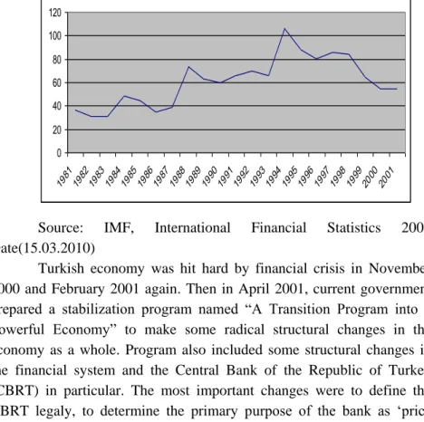
Turkey also lived energy and exchange crisis at the end of 70‟s and economical instability in the same era. Inflation rate reached 52,6% level in 1978 and it went beyond 100% level in 1980. Through the agency of economical crisis, inflation rate increased over 100% level in
1994 again. Because of full-fledged recessions, high inflation rates had become permanent for the Turkish economy. Movements of inflation in this period, between 1981 – 2001, can be seen in the following graphic number 1.
Graphic 1. Inflation Rate 1981-2001 Period
0 20 40 60 80 100 120 198119821983198419851986198719881989199019911992199319941995199619971998199920002001
Source: IMF, International Financial Statistics 2009 Date(15.03.2010)
Turkish economy was hit hard by financial crisis in November 2000 and February 2001 again. Then in April 2001, current government prepared a stabilization program named “A Transition Program into a Powerful Economy” to make some radical structural changes in the economy as a whole. Program also included some structural changes in the financial system and the Central Bank of the Republic of Turkey (CBRT) in particular. The most important changes were to define the CBRT legaly, to determine the primary purpose of the bank as „price stability‟ and to begin inflation targeting program. In this context exchange rates would be determined by competitive exchange market anyway.
After a short period from the beginning of stabilization program, early general elections was called and another government has came to office in november 2002. Although change in government and management of economy, present government announced that it would continue to practice stabilization program as strong as past government. So inflation targeting program has continued in the same path also.
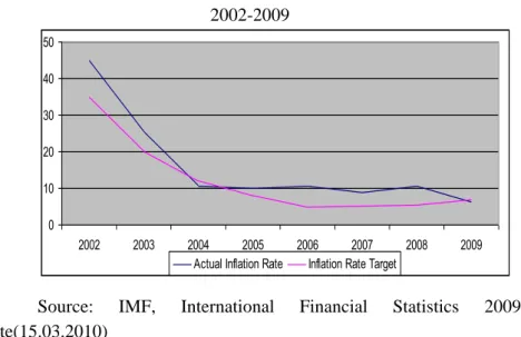
Inflation rate started to run low and it was only one digit rate after several decades in Turkish economy in 2004.
Graphic 2. Actual Inflation Rate and Inflation Target Period
2002-2009 0 10 20 30 40 50 2002 2003 2004 2005 2006 2007 2008 2009
Actual Inflation Rate Inflation Rate Target
Source: IMF, International Financial Statistics 2009 Date(15.03.2010)
The main goal of our paper is to understand whether short term interest rate which is used as an instrument of monetary policy, is effective instrument to success price stabilization during economical stabilization program and to examine importance of output in the program by using Taylor type monetary policy reaction function. Because studies about developed countries have had some suggestions about usefulness of short term interest rate, if it is used together with inflation targeting policy to achieve price stability and to establish stable production level and about that it is more effective than other monetary policy instruments (Money supply, exchange rate, etc.) (Kesriyeli; 1998).
We examine inflation targeting period to understand behaviour of short term interest. So time interval considered in this study differs from other studies about Turkish economy. Another important difference in this study that we take into account extended monetary policy reaction function by including exchange rate into the reaction function. Lastly although there are plenty of studies about Taylor rule, a few of them used VAR methodolgy to examine Taylor rule. By using VAR analysis, we will be able to consider possible simultaneous relationship among the endogenous variables and to avoid simultaneity bias.
In the second part of the study Taylor rule will be introduced in a nutshell. National and international literature will be overwieved in the third part. Information about data used in this study and model established through econometrical analysis will be investigated in the fourth part of the paper. Fifth part is about empirical results and at the end of our study we give useful insight about Turkish inflation targeting program and compare monetary policy reaction derived by econometrical application with original monetary policy reaction of Taylor represented his announcement in 1993.
2. Taylor Rule
John B. Taylor (1993a) offered a different monetary policy rule has dynamic pattern and put in a plan to practice monetary policy rules. That is why starting by examining his proposals about characteristics of a rule and about how it might be practiced will be plausible explanation, before we describe his monetary policy reaction function. According to Taylor monetary authority does not need to follow mechanically any algebraic formula to practice monetary policy rule. Also authority does not need to install a constant rule. It means instrumental variable does not cost certain value. Taylor (1993b) emphasized to not to confuse discretionary policy practice and his proposal because of these ideas. Because practicing a policy rule needs responsibility and judgement, so computers can not achieve it and so weigh of variables can change according to situation of economy. Last point is that if a policy rule is to have any meaning, it must be in place for a reasonably long period of time. For a policy rule, several business cycles would certainly be sufficient, but, for many purposes, several years would do just as well (Taylor; 1993b; 5).
According to Taylor, the term “policy rule” connotes either a fixed setting for the policy instruments or a simplistic mechanical procedure (Taylor; 1993a; 198). So an alternative terminology “systematic policy” was offered by Taylor has better explanation power which he try to imply.
Policy rule proposal of Taylor is that short term nominal interest rate react according to change in inflation rate from its target introduced by policy makers and actual GDP from potential GDP. If inflation rate deviates higher than target or GDP gap rises positively, short term nominal interest rates will increase and it will decrease if actual inflation
rate is below its target or actual GDP falls under its potential. So in equilibrium short term nominal interest rate inflation will be on target and all of sources possible for production in economy will be material in process of production. We can express relationship between variables by developing an equation. We can note variables as follows:
i
Short term interest rate
f
i
Real interest rate
Actual inflation rate
*
Target inflation rate
h
Inflation rate reaction coefficient
y
Actual GDP or GDP growth rate
*
y
Potantial GDP or potential GDP growth rate
g
GDP gap reaction coefficientAfter notation of variables used in policy reaction function, we can write equation as follows:
*
* * y y y g h i i f
(1)As can be seen in this equation, while actual inflation is equal to inflation target and output level is equal to its potential, short term nominal interest rate will be equal to sum of real interest rate and actual inflation. So there will be no importance of values of coefficients
g
andh
. If actual inflation rate rises, short term inflation rate will increase vice versa. Effect of increase in inflation will be determined according to size of coefficienth
. If it is between 0 and 1, increase in interest rate will be less than change in inflation and if it is more than 1, increase will be bigger than inflation change.g
coefficient size will determine reaction size of interest rate when output differs from its potential like coefficienth
.Sizes of coefficients h and
g
show preferences of policy makers about which goal is important for them. This is because they represent Monetarist and Keynesian policy proposals those contrast entirely. Namely if coefficientg
is valued zero and coefficienth
is valued high, it can named as pure Monetarist rule. So monetary authority takes only onboard deviations in inflation and neglect output gap. If coefficient
h
is zero and coefficientg
is valued high, it can be named as pure Keynesian rule. In such a case monetary authority only consider unemployment and neglects deviations in inflation (Akat; 2004; 7).Taylor‟s original analysis in his original paper in 1993 does not include exchange rate. Because he analysed U.S.A. economy in a closed economy model and Taylor (2001) pointed out that there are some indirect effects of exchange rate on interest rate. Because of this reason to determine response of interest rate to a shock in exchange rate is hard (Taylor; 2001; 264). But it is useful to include exchange rate into the reaction function especially for emerging economies which exchange rate has high pass through into prices. Ball (1999), Svensson (2000) and Taylor (2001) placed exchange rate into policy reaction function and found that exchange rate has significant coefficient. So it would be useful to include exchange rate variable for Turkey that has open economy and where exchange rates float into competitive market.
3. Literature
Taylor rule and estimating Taylor-type monetary policy reaction function were research bases for several studies for last decade and most of them took into account industrialized economies specially U.S.A., European Union and Japan. These studies estimated monetary policy reaction function by using different econometrical methodologies in different time periods and they added different variables into reaction function. Although there is a vast literature about Taylor rule, we mention some basic studies estimating Taylor-type monetary policy reaction function for industrialized economies in our study.
One of them belongs to Judd and Rudebusch (1998). They examined U.S.A. economy and parted period, between 1970 and 1997, according to chairmenship of Federal Reserve System and followed error correction model (ECM) for econometric analysis. At the end of the study they implied that behaviour of FED differs according to chairman of it. So, while Greenspan followed Taylor-type monetary policy, Volker and Burns did not consider Taylor rule.
Bernanke and Gertler (1999) added asset prices into Taylor‟s policy rule reaction function and examined U.S.A. and Japanese economies between 1979 and 1997. They built up Bernanke, Getrler and Gilchrist model and simulate economy by using the generalized methods
of moments (GMM) with correction for MA(12) autocorrelation. They implied useful framework for explaining U.S.A. monetary policy actions at the end of their studies.
Clarida, Gali and Gertler (1997) examined six countries into two different groups to estimate monetary policy reaction function for each group. First group consisted of Germany, Japan and U.S.A., another group consisted of United Kingdom, France and Italy. They estimated monetary policy reaction function for post-79 era by using the generalized methods of moments (GMM) and they concluded that first group countries take into account anticipated inflation in their monetary policy reaction function instead of lagged inflation like original study of Taylor. In another study of Clarida, Gali and Gertler (2000) modified Taylor rule by smoothing interest rate and estimate forward looking monetary policy reaction function for Volcker-Greenspan period. They used same methodology and they concluded that interest rate policy is more sensitive to changes in expected inflation than before Volcker period.
Levin, Wieland and Williams (1998) estimated monetary policy reaction function for U.S.A. economy also by using four different structural macroeconometric model and compared results of each model. They examined U.S.A. data belonging years between 1980-1996 by using a combination of OLS, 2SLS and GMM methodologies. They concluded that models include first difference of the federal fund rate work better. Because first difference of the rate responds to the current output gap and the deviation of the one year avarage inflation rate from target.
Florens, Jondeau and Bihan (2001) estimated monetary policy reaction function for Federal Reserve of U.S.A. (FED) in a different methodology. They estimated forward looking reaction function period including years between 1979 and 1998 and they used the maximum likelihood (ML) method instead of the generalized methods of moments (GMM) different from Clarida, Gali and Gertler (1998). Then, they compared results with GMM and two step GMM method results and implied that ML methodology gives more robust results than GMM methodology to estimate policy reaction function of FED.
Jamal and Hsing (2007) estimated policy reaction function for FED by using quarterly data belonging years between 1987 and 2005 including Greenspan period as a chairman of FED. They put real interest
rate, inflation target, output gap, inflation rate and federal fund rate into function and estimated by Newey-West methodology. They got results supporting significancy of Taylor rule and implying that coefficients of rule differ from Taylor‟s original rule. As a result they concluded that constant term and inflation term is not different from Taylor‟s original study and but coefficient of output gap is different from Taylor‟s finding. According to them FED gave less importance to changes in output gap.
Mehra and Minton (2007) estimated policy reaction function for Greenspan also. They estimated policy reacition function in a forward looking structure and assumed bank was smoothing interest rate. They took into account core inflation and estimated function by using the generalized methods of moments (GMM). They also compared data whether real time data gives more robust results rather than revised data. According to results of their analyse, Greenspan followed Taylor rule and reaction function responded changes in inflation strongly and weakly to output gap compare to inflation.
Leigh (2008) estimated Taylor type policy reaction function by using the maximum likelihood (ML) method to analyse 1979-2004 period including Volcker and Greenspan. They relaxed assumption that the inflation target is constant over the time and they assumed variation in implicit inflation target by using Kalman filter. He concluded that FED followed time varying implicit inflation targeting procedure significantly.
Cote et. al (2004) analysed Canada economy to examine performance and robustness of simple policy rules for the Canadian economy. They compared performances of seven different policy rule by using the vector autoregression (VAR) methodology. They found that adding exchange rate term to a simple policy rule often increases the value of policymaker‟s loss function and open economy rules do not perform well in many models. Although it was not robust, they found that a simple nominal Taylor type rule that has a coefficient of 2 on the inflation gap and 0,5 on the output gap performs better.
Carstensen (2006) put nominal and real exchange rates into original function of Taylor rule to examine behaviour European Central Bank (ECB) period between 1996 and 2006. He concluded that bank does not take into account inflation in its policy decisions and so it is not possible to construct Taylor type policy reaction function for it in these years. Gorter, Hacobs and de Haan (2008) included inflation and output
gap expectations into model and analysed period between 1991 and 2003. They applied the non-linear least squares and generalized methods of moments (GMM) and they compared results of each methodology. They found that ECB uses expected inflation and expected output growth in its interest rate decisions, also coefficient of realized inflation is not significant in conventional reaction function model.
Hsing (2004) estimated monetary policy reaction function of Bank of Japan in his study. He used overnight call rate as short term interest rate. Then he added financial variables, stock prices and exchange rate, into reaction function and used quarterly data belonging 1979 and 2002. He estimated policy reaction function by using the vector autoregressive (VAR) methodology. At the end of his empirical analysis he implied that overnight call rate reacts positively to a shock to the output gap, the inflation gap, yen depreciation, stock prices. The response of the overnight call rate to yen depreciation on stock prices lasts longer. Lastly, the reaction of the call rate to the inflation gap goes on longer than that of the overnight call rate to the output gap.
Although there is a vast literature concerning industrialized countries, number of studies investigating emerging countries were limited. But the number of these studies have started to rise in recent years. Turkish economy has been subject to studies about Taylor rule and estimating monetary policy reaction function also. In one of them Kesriyeli and Cihan (1998) estimated backward and forward looking monetary policy reaction function by using two stage least squares methodology. They took into account years between 1987 and 1998 and concluded that Taylor type policy reaction function is a useful guide for countries which has stable and low inflation rate instead of emerging countries have unstable economies and high inflation.
Us (2004) examined Turkish monetarial transmission mechanism in a small structural model and compared Taylor rule and monetary condition index (MCI) in her study. She estimated impulse response functions for each rule by the vector autoregressive (VAR) methodology. At the end of her study, she found that monetary condition index is effective to stabilize economy and reduce fluctuations in economy and so policymakers ought to use MCI while they decide policy actions.
Caglayan (2005) used the multinominal logit model to examine whether inflation rate and output gap are important indicator of short term interest
rate decisions. She used data belonging years between 1990 and 2004. As a result of this analysis, she implied that inflation rate is an important indicator and but output gap is not important for policymakers. Caglayan also suggested that lagged output gap might be used as an alternative component of interest rate decisions.
Aklan and Nargelecekenler (2008a) analysed period between 2002 and 2006 to see whether the CBRT followed Taylor rule in these years as a monetary policy benchmark. They estimated policy reaction function by using the generalized methods of moments (GMM). At the end of their study they implied that interest rate reacts inflation rate, output gap and also exchange rate in the context of Taylor rule. They examine the Turkish economy in another article (2008b) with the data belonging 2001-2006 years. They estimated Taylor type policy reaction function as backward and forward by using same methodology. At the end of their study, they found that Taylor rule is current for the Turkish economy and they implied that after 2001 crisis, coefficients of inflation rate and output gap are bigger than before.
4. Data, Model and Methodology 4.1. Data
Stabilization program has been started in april 2001 in Turkey and the CBRT has started to announce inflation targeting by 2002. Also positive results of program appeared in the first month of 2002 on inflation and other macroeconomic variables. For these reasons we started to examine inflation targeting era by the first month of 2002 and we used data covering the period 2002:01-2009:11 in order to see results of program.
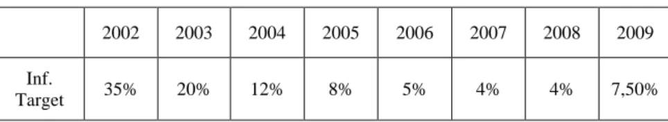
All of data used in analysis were obtained from publication of the International Money Fund named International Financial Statistics. We used interbank interest rate as short term nominal interest rate. Inflation rate was measured as the first difference of CPI (2005=100) and deseasonalized by using TRAMO/SEATS program. Then inflation gap was calculated as the difference between actual inflation and backward inflation target announcement of the CBRT‟s webiste. Inflation targets for each year can be seen in table 1.
Table 1. Inflation Target per year
2002 2003 2004 2005 2006 2007 2008 2009 Inf.
Target 35% 20% 12% 8% 5% 4% 4% 7,50%
Source: The CBRT. www.tcmb.gov.tr Date: 25.03.2010
We deseasonalized industrial production index by using TRAMO/SEATS program to derive potential output by HP filtre and we obtained output gap by calculating difference between potential output and actual output. We used SDR to measure exchange rate where the SDR is an international reserve asset, created by the IMF in 1969 to supplement its member countries‟ official reserves. Its value is based on a basket of four key international currencies are euro, U.S. Dollar, Pound Sterling and Japanese Yen, and SDRs can be exchanged for freely usable currencies (IMF; 2010; 1). Inflation rate and SDR data were used in logharitmic forms.
Table 2: The Data Set
Variables Explanations Resources INT Interbank Interest Rate IFS INFGAP Inflation Rate Gap Derived from CPI (2005=100) IFS GAP Output Gap (Derived by HP filtering process) IFS SDR Special Drawing Right IFS
4.2. Model and Methodology
We can write original Taylor rule function as below: INT=f(INF, GAP, GAP) (2)
We extend function as an open economy analysis by including SDR into function,
INT=f(INF, GAP, SDR) (3)
Some of these variables might have relationships. For instance, after the CBRT lowers on interest rates, consumption and investment would increase, thus aggregate demand would shift higher level and so GDP would increase. So it would change output gap positively. At the same time an increase in output would cause a decrease unemployment rates and inflation rate would increase. Because of the practicing VAR
methodology and all the right hand side variables are identical and lagged, simultaneity bias is not concerned. It is essentially a system of equations whose dependent variables are regressed on lagged observations of all the variables in the system (Ford: 1986: 2).
In VAR framework, there are no exogenous variables and no identifying restrictions. The only role for economic theory is in specifying the variables to be included (McCoy: 1997: 2). In VAR methodology, each time serie has to be stationary to include into analysis. Therefore, before including a variable into system, it is important to control stationarity.
We can write system of simultaneous equations in a vector form as follows.
t t
t
B
L
y
C
Ay
(
)
1
(4)This is a general representation where
y
t is a vector ofendogenous variables,
y
t1 is a vector of their lagged values, and
t is awhite noise vector of the disturbance terms for each variable.
A
is an
n
square matrix and n is the number of variables that contains the structural parameters of the contemporaneus endogenous variables.)
(L
B
is apth
degree matrix polynomial in the lag operator L, wherep
is the number of lagged periods used in the model. C is a square matrix sized nn, contains the contemporaneous response of the variables to the disturbances or innovations.
McCoy (1997) mentioned that there is a problem with presentation in eq 1., because the coefficients in the matrices are unknown and variables have contemporaneous effects on each other. So it is not possible to determine the values of the parameters in the model. To fully identify model, it is possible to transform into a reduced-form model to derive the standart VAR representation in the following equation.
t t t
D
L
y
e
y
(
)
1
(5)In this form, D(L)equals to
A
1B
(
L
)
ande
t equals to tC
A
1
. The last term in equation is serially uncorrelated (Ioannidis: 1995: 256). The matrix is the variance/covariance of the estimated residuals,e
t, of the standart VAR.2 2 1 2 2 2 2 1 1 1 2 2 1 ... ... ... ... ... ... ... ... ... ... ... ... ... ... ... ... n n n n n
In this matrix ,there are
(
n
2
n
)
/
2
number of restrictions requried to identify to system. Traditional VAR methodology proposes the identification restrictions based upon on a recursive structure known as Cholesky decomposition (Ioannidis: 1995: 256). Cholesky decomposition seperates the residualse
t into orthogonal shocks byrestrictions imposed on the basis of arbitrary ordering of the variables and implies that first variable responds only to its own exogenous shocks, second responds to first variable „s and its own exogenous shocks. So the structure of matrix will be lower triangular, where all elements above the principial diagonal are zero (McCoy: 1997: 5).
After the identification of restrictions impulse response function (IRF) is employeed to reflect the dynamic effect of each exogenous variable response to the individual unitary impulse from other variables. The IRF can explain the current and lagged effect over time of shocks in the error term (Liu: 2008: 243).
The variance decomposition is another test in the VAR analysis. Variance decomposition gives information about dynamic structure of system. The main pupose of variance decomposition is to introduce effects of each random shock on prediction error variance for future periods ( Ozgen and Guloglu: 2004: 9).
5. Empirical Results
A stationary time serie is significant to a regression analysis based on time series. A nonstationary time serie would lead to a spurious regression. For this reason series must be stationary to include into VAR analysis. To determine whether the series are stationary, the augmented Dickey-Fuller (1979) unit root tests are applied. Table below summarizes the results of ADF test for all the variables.
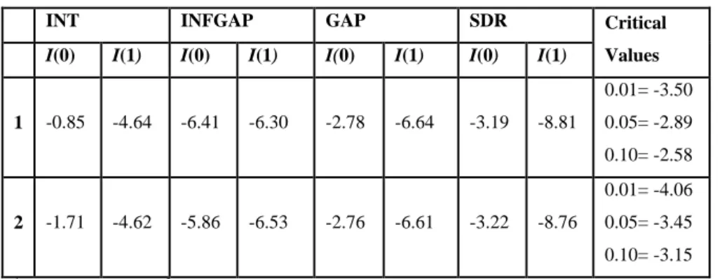
Table 3. ADF Unit Root Test of Results
INT INFGAP GAP SDR Critical
Values
I(0) I(1) I(0) I(1) I(0) I(1) I(0) I(1)
1 -0.85 -4.64 -6.41 -6.30 -2.78 -6.64 -3.19 -8.81 0.01= -3.50 0.05= -2.89 0.10= -2.58 2 -1.71 -4.62 -5.86 -6.53 -2.76 -6.61 -3.22 -8.76 0.01= -4.06 0.05= -3.45 0.10= -3.15 1
Intercept (c) term; 2 Trend (t) and intercept (c) term.
Note: MacKinnon (1996) critical values was used. All variables was made ADF test according to Schwarz information criterion.
Table 3 shows the unit root test results of variables by using the ADF unit root test. The null hypothesis of non-stationary was performed at the 1% significance levels. Results show that inflation gap variable is stationary at level. But interest rate, output gap rate and exchange rate variables have unit roots at level. These variables are found to be stationary only when tested at first difference. Output gap rate, interest rate and exchange rate variables are included into model with their first differences I(1), while inflation gap variable is included into model with its level I(0).
One of the important question in the VAR models is to select the optimal lag length. The most common and simple approach in selecting exact lag length is to re-estimate VAR model until the smallest Akaike Information criterion (AIC) value is found. Because comparing two or more models, the model with the lowest AIC is preffered (Gujarati: 2004: 537). According to Asteriou (2005) the judgement of the optimal length should still take other factors into account: For example autocorrelation, heteroskedasticity, possible ARCH effects and normality of residuals. In this study we choosed two lags based on Akaike information criterion and results can be seen in appendice A.
Another important question is the stability of the VAR model in order to get valid results from impulse response analysis. Stability would be achieved if the characteristic roots of the matrix coefficients have a modulus less than one. So we tested lag structure and stability of the number of lag length with autocorrelation test and had a look at unit root
graph. Graph showed that all roots are less than one and no roots are out of the unit circle. In autocorrelation test results imply that there is no autocorrelation. Autocorrelation test results and unit root graph are given in appendice B.
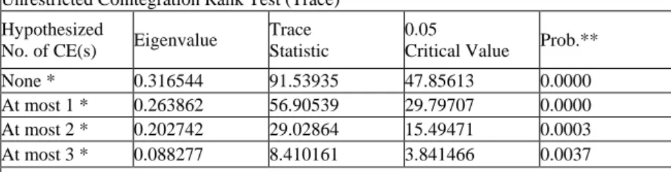
We practiced Johansen cointegration analysis to check long term relationship between variables. We found that there are four cointegrating relationship between variables according to Trace test and four cointegrating relationship according to maximum eigenvalue test. So the test rejected null hypothesis suggests there is no cointegrating relationship among variables at level 5%. This means VAR analysis fits best to analysis. Test results can be seen in table 4.
Impulse response function derived from the VAR analysis is useful to trace out response of one variable to a shock in the error term of another variable. It can explain current and lagged effect over time of shocks in the error term (Liu et. al: 2008: 243). For this reason impulse response function is one of the important element of the VAR analysis.
Table 4. Johansen Cointegration Analysis (Trace and Maximum
Eigenvalue Tests)
Unrestricted Cointegration Rank Test (Trace) Hypothesized
No. of CE(s) Eigenvalue
Trace Statistic
0.05
Critical Value Prob.** None * 0.316544 91.53935 47.85613 0.0000 At most 1 * 0.263862 56.90539 29.79707 0.0000 At most 2 * 0.202742 29.02864 15.49471 0.0003 At most 3 * 0.088277 8.410161 3.841466 0.0037 Trace test indicates 4 cointegrating eqn(s) at the 0.05 level
* denotes rejection of the hypothesis at the 0.05 level **MacKinnon-Haug-Michelis (1999) p-values
Unrestricted Cointegration Rank Test (Maximum Eigenvalue) Hypothesized
No. of CE(s) Eigenvalue
Max-Eigen Statistic
0.05
Critical Value Prob.** None * 0.316544 34.63396 27.58434 0.0002 At most 1 0.263862 27.87676 21.13162 0.0635 At most 2 0.202742 20.61848 14.26460 0.0737 At most 3 * 0.088277 8.410161 3.841466 0.0047 Max-eigenvalue test indicates 4 cointegrating eqn(s) at the 0.05 level
* denotes rejection of the hypothesis at the 0.05 level **MacKinnon-Haug-Michelis (1999) p-values
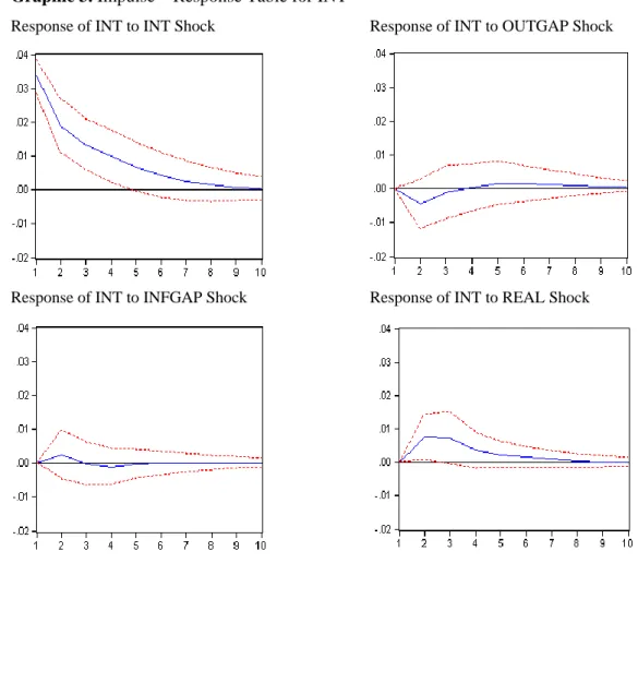
Graphic 1 presents the impulse response functions of the interest rate for a year. Within 95% confidence interval, INT has positive response to a shock to INFGAP, SDF and lagged INT significantly and negative response to a shock to OUTGAP significantly. This result can be interpreted as the CBRT would increase short term nominal interest rate if inflation rate goes beyond target level or exchange rate increases and would decrease it if actual output passes output target at the begining of the shock.
There are a number of point to deliberate. First of all short term nominal interest rate responses inflation gap positively in first three months, then effect turns negative and dies out in five months. Response of short term nominal interest rate to output gap rate is negative in first three months and then it turns to positive. It continues untill the end of the period examined. Response of short term nominal interest rate to exchange rate is positive and effective for more than six months. These mean that the CBRT reacts, if actual inflation passes inflation target and the bank increases short term nominal interest rate appropriately with the rule. Meanwhile a positive shock in output gap rate would affect interest rate negatively in first months and but it would turn to positive later. Behaviours of the CBRT differs from the rule at this point. This means short term nominal interest rate is more concerned with inflation targeting and less concerned with output gap rate. Positive response of the CBRT to SDR can be interpreted as fear of floating effect. Increasing exchange rate would cause an increase in actual inflation and it would affect inflation targeting regime.
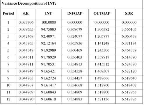
In order to extract effects of each variable on short term nominal interest rate, variance decomposition method was used. As can be seen in the table 6, lagged values of interbank interest rate are the most influental variable, it can explain more than 90% at the end of a year. Inflation gap can explain variation in interbank interest rate just a little portion of it and it is not more than1%. Output gap rate can explain up to 1,5% of variance. SDR‟s explanation capability is up to 6,5% also.
Graphic 3. Impulse – Response Table for INT
Response of INT to INT Shock Response of INT to OUTGAP Shock
Table 5. Variance Decomposition of Overnight Interest Rate Variance Decomposition of INT:
Period S.E. INT INFGAP OUTGAP SDR
1 0.033706 100.0000 0.000000 0.000000 0.000000 2 0.039655 94.75883 0.368679 1.306382 3.566105 3 0.042468 92.40971 0.324077 1.205777 6.060438 4 0.043763 92.12164 0.365936 1.141248 6.371174 5 0.044348 91.92989 0.360469 1.245306 6.464339 6 0.044611 91.78929 0.356403 1.339917 6.514390 7 0.044711 91.70531 0.354813 1.415512 6.524370 8 0.044749 91.65421 0.354358 1.469307 6.522120 9 0.044763 91.62724 0.354457 1.498666 6.519640 10 0.044767 91.61417 0.354668 1.512760 6.518402 11 0.044769 91.60843 0.354809 1.518800 6.517965 12 0.044770 91.60610 0.354883 1.521126 6.517895 6. Conclusion
In this study, we aim to extend Taylor rule and applied VAR methodology to examine the monetary policy reaction function of the CBRT. Results can be interpreted as follows. Short term nominal interest rate responses significantly to inflation gap, output gap rate and exchange rate. Response of short term nominal interest rate to exchange rate is positive and expected as in Taylor (2001), Ball (1999) and Svensson (2000) findings.
Response of short term interest rate to inflation gap is positive and but it continues for a little while. Direction of the response is as expected in original rule. Response of short term nominal interest rate to output gap rate is negative. It is in the opposite direction with the original rule. Although interest rate responses to shocks in these variables, variables could explain only a little portion of variance in interest rate. ıt is not more than 10% at the end of year.
According to impulse response analysis and variance decomposition process, monetary policy reaction function differs from Taylor‟s monetary policy reaction function and emphasizes on inflation gap. Output gap rate does not takes place in function as expected. This
also consistent with remarks and actions of the CBRT. Because the CBRT has announced its first goal as price stabilization after the beginning of stabilization program and made some regulations to provide bank‟s freedom and to prevent government‟s effects on price stabilization goal.
According to results captured from impulse response analysis and variance decomposition process, interbank interest rate responses shocks in inflation gap, exchange rate and output gap rate significantly. Also inflation gap, exchange rate and output gap rate can explain a little part of variance on interest rate. So we imply that Taylor type monetary policy reaction function might be a part of decision making process of the CBRT to adjust short term nominal interest rate. Also there might be some other instruments help inflation targeting. This implications support John B. Taylor‟s first advice about practicing systematic monetary policy that we have mentioned in introduction. Extending monetary policy reaction function might be research topic for further economic analysis.
REFERENCES
Aklan, N.A. and Nargelecekenler, M. (2008a) “Taylor Rule in Practice: Evidence from Turkey” International Advanced Economic Resources, 14, 156-166.
Aklan, N.A. and Nargelecekenler, M. (2008b). “Taylor Kurali: Turkiye Uzerine Bir Degerlendirme” Ankara Universitesi SBF Dergisi, 63(2), 21-40.
Asteriou, D. (2005). “Applied Econometrics: A Modern Approach Using Eviews and Microfi“ Palgrave Macmillan, New York.
Ball, L. (1999).“Policy Rules for Open Economies” in John B. Taylor ed., Monetary Policy Rules, University of Chicago Pres, Chicago, pp. 127-144.
Bernanke, B. and Gertler, M. (1999). “Monetary Policy and Asset Price Volatility” Federal Reserve Bank of Kansas City Economic Review, 16-50.
Caglayan, E. (2005). “Turkiye‟de Taylor Kurali‟nin Gecerliliginin Ekonometrik Analizi” Marmara Universitesi I.I.B.F. Dergisi, 20(1).
Carstensen, K. (2006). “Estimating the ECB Policy Reaction Function” German Economic Review, 7(1), 1-34.
Clarida, R., Gali, J., Gertler, M. (1997). “Monetary Policy Rules in Practice: Some International Evidence” National Bureau of Economic Research Working Paper, no. 6254.
Clarida, R., Gali, J., Gertler, M. (2000). “Monetary Policy Rules and Macroeconomic Stability Evidence and Some Theory” The Quarterly Journal of Economics, 115(1), 147-180.
Cote, D., Kuszczak, J., Lam, J.P., Liu, Y., Amant, S.P. (2002). “The Performance and Robustness of Simple Monetary Policy Rules in Models of the Canadian Economy” Canadian Journal of Economics, 37(4), 978-998.
Dickey, D.A., Fuller W.A. (1979). “Distribution of the Estimators for Autoregressive Time Series with a Unit Root”, Journal of The American Statistical Association, 74.
Florens, C., Jondeau, E., Bihan, H.L. (2001). “Assessing GMM Estimates of the Federal Reserve Reaction Function” Universite Paris XII Val de Marine Publications, Paris.
Ford, S. (1986). “A Beginner‟s Guide to Vector Autoregression” Staff Paper no. P86-28, University of Minnesota Institute of Agriculture, Forestry and Home Economics, St. Paul.
Friedman, I.S. (1980). “Inflation A World-wide Disaster” Houghton Mifflin Company, Boston.
Gujarati, D.N. “Basic Econometrics, Fourth Edition” McGraw-Hill Companies, New York.
Haberler, G. (1966). “Inflation, Its Causes and Cures; with a New Look Inflation in 1966” American Enterprise Institute for Public Policy Research, Washington.
Hsing, Y. (2004). “Estimating the Bank of Japan‟s Monetary Policy Reaction Function” Banca Nazionale Del Lavoro Quarterly Review, 57, 169-183.
Ioannidis, C., Laws, J., Matthews, K., Morgan, B. (1995). “Business Cycle Analysis and Forecasting with a Structural Vector Autoregression Model for Wales” Journal of Forecasting, 14, 251-265.
Jamal, A.M.M., Hsing, Y. (2007). “Test of The Taylor Rule and Policy Implications” International Atlantic Economic Society Journal, 35, 121-122.
IMF (2010). “Special Drawing Rights” International Money Fund Fact Sheet, Washington.
Judd, J.P., and Rudebusch, G.D. (1998). “Taylor‟s Rule and the Fed: 1970-1997” FRBSF Economic Review, no.3, 3-16.
Kesriyeli, M. and Yalcin, C. (1998). “Taylor Kurali ve Uygulamasi Uzerine Bir Not” CBRT Discussing Paper, no. 9802.
Leigh, D. (2008). “Estimation the Federal Reserve‟s Implicit Inflation Target: A State Spave Approach” Journal of Economic Dynamics & Control, 32, 2013-2030.
Levin, A., Wieland, V., Williams, J.C. (1998). “Robustness of Simple Monetary Policy Rules Under Model Uncertainity” Board of Governers of the Federal Reserve System, Washington.
Liu, C., Luo, Z.Q., Ma, L., Picken, D. (2008). “Identifying House Price Diffusion Patterns Among Australian State Capital Cities” International Journal of Strategic Propoerty Management, 12, 237-250.
McCoy, D., (1997). “How Useful is Structural VAR Analysis for Irish Economics” Eleventh Annual Conference of the Irish Economic Association, Athlone.
Mehra, Y.P., Minton, B.D. (2007). “A Taylor Rule and the Greenspan Era” Economic Quarterly, 93(3), 229-250.
Ozgen, F.B., Guloglu, B. (2004). “Analysis of Economic Effects of Domestic Debt in Turkey Using VAR Technique” METU Studies in Development, 31, 93-114.
Svensson, L.A.O. (2000). “Open Economy Inflation Targeting” Journal of International Economics, 50(1), 155-183.
Taylor, J.B. (1993). “Discretion Versus Policy Rules in Practice” Carnegie-Rochester Conference Series on Public Policy, 39, 195-214.
Taylor, J.B. (1993). “Macroeconomic Policy in a World Economy: From Econometric Design to Practical Operation” W.W. Norton & Company, New York.
Taylor, J.B. (2001). “The Role of The Exchange Rate in Monetary Policy Rules” The American Economic Review, 91(2), 263-268.
Us, V. (2004). “Monetary Transmission Mechanism in Turkey Under The Monetary Conditions Index: An Alternative Policy Rule” Applied Economics, 36, 967-976.
Wilson, G.W., (1982). “Inflation-Causes, Consequences and Cures” 1st edition, Indiana University Pres, Bloomington.
Appendices A
VAR Lag Order Selection Criteria
Lag LogL LR FPE AIC SC HQ
0 333.1390 NA 3.83e-09 -8.027781 -7.910380 -7.980646 1 442.9204 206.1749 3.90e-10* -10.31513 -9.728128* -10.07946* 2 458.9931 28.61724* 3.90e-10 -10.31691* -9.260297 -9.892694 3 465.8706 11.57422 4.91e-10 -10.09440 -8.568192 -9.481653 4 475.8950 15.89236 5.76e-10 -9.948658 -7.952842 -9.147369 5 481.8730 8.894063 7.51e-10 -9.704219 -7.238799 -8.714390 6 497.4992 21.72425 7.84e-10 -9.695102 -6.760078 -8.516735 7 509.7756 15.86949 9.00e-10 -9.604282 -6.199655 -8.237376 8 520.0157 12.23824 1.11e-09 -9.463798 -5.589567 -7.908354 9 526.1741 6.759173 1.53e-09 -9.223758 -4.879924 -7.479775 10 543.8882 17.71412 1.65e-09 -9.265566 -4.452128 -7.333044 11 558.3747 13.07316 1.99e-09 -9.228651 -3.945609 -7.107590 12 579.5279 17.02577 2.12e-09 -9.354339 -3.601693 -7.044740 * indicates lag order selected by the criterion
LR: sequential modified LR test statistic (each test at 5% level) FPE: Final prediction error
AIC: Akaike information criterion SC: Schwarz information criterion HQ: Hannan-Quinn information criterion
Appendices B -1.5 -1.0 -0.5 0.0 0.5 1.0 1.5 -1.5 -1.0 -0.5 0.0 0.5 1.0 1.5
Autocorrelation Test
Lag 1 Lag 2 Lag 3 Lag 4
LM-Stat Prob LM-Stat Prob LM-Stat Prob LM-Stat Prob 30.774 0.0144 15.787 0.4679 13.738 0.6182 7.6273 0.9592 19.262 0.2553 18.035 0.3218 15.326 0.5009 13.460 0.6388 14.392 0.5695 14.010 0.5979 10.622 0.8321 8.1459 0.9444 16.013 0.4520 17.137 0.3768 16.747 0.4021 9.4075 0.8957 7.5218 0.9618 10.930 0.8138 12.490 0.7096 10.838 0.8193 17.035 0.3833 22.781 0.1197 21.757 0.1512 19.023 0.2675 12.928 0.6780 12.358 0.7190 15.865 0.4624 13.915 0.6050 4.5219 0.9977 4.4828 0.9978 2.8436 0.9999 4.7516 0.9969 19.170 0.2599 16.523 0.4171 8.1613 0.9439 11.242 0.7943 14.620 0.5526 9.5601 0.8886 11.910 0.7501 14.385 0.5700 11.330 0.7887 12.163 0.7326 10.108 0.8609 12.235 0.7276 39.083 0.0011 34.345 0.0049 34.029 0.0054 33.215 0.0069