2 71
13
A
N
I
NTEGRATED
R
EPLENISHMENT
AND
T
RANSPORTATION
M
ODEL
Computational Performance Assessment
R A M E Z K I A N, E M R E BER K , A N D
Ü LK Ü GÜ R L ER
13.1 Introduction
Transformation processes with multiple inputs typically exhibit non-linearities in their output with respect to input usages. They have been traditionally modeled via production functions in the microeconomics literature (Heathfield and Wibe, 1987). One of the most common pro-duction functions is the Cobb–Douglas (C–D) propro-duction function. This production function assumes that multiple (n) inputs (also called factors or resources) are needed for output, Q, and they may be substi-tuted to take advantage of the marginal cost differentials. In general, it has the form Q A xi
i n i , = ⎡⎣ ( )⎤⎦ =
∏
α1 where A represents the total factor
productivity of the process given the technology level, x(i) denotes the
amount of input i used, and αi > 0 is the input elasticity. The total
Contents 13.1 Introduction 271 13.2 Model 274 13.2.1 Assumptions 274 13.2.2 Formulations 276 13.3 Numerical Study 279 13.3.1 Overall Assessment 280 13.3.2 ANOVA Assessment 282 Acknowledgment 287 References 287
elasticity parameter r i m i = ⎛ ⎝ ⎜ ⎜ ⎜ ⎞ ⎠ ⎟ ⎟ ⎟ =
∑
1 1αmay be greater than (smaller than) or equal to 1 depending on whether there is diminishing (increasing) returns to resources, resulting in convex (concave) operational costs. The C–D production function was first introduced to model the labor and capital substitution effects for the US manufacturing industries in the early twentieth century (Cobb and Douglas, 1928). Despite its macroeconomic origins, since then, it has been widely applied to indi-vidual transformation processes at the microeconomic level, as well. For example, the C–D production function was employed to model production processes in the steel and oil industries by Shadbegian and Gray (2005) and in agriculture by Hatirli et al. (2006). Logistics activi-ties associated with shipment preparation, transportation/delivery, and cargo handling also use, directly and/or indirectly, multiple resources such as labor, capital, machinery, materials, energy, and information technology. Therefore, it is not surprising that there is a growing lit-erature on the successful applications of the C–D-type production functions to model the operations in the logistics and supply chain management context. Chang’s (1978) work seems to be the earliest to construct a C–D production function to analyze the productivity and capacity expansion options of a seaport. Rekers et al. (1990) esti-mate a C–D production function for port terminals and specifically model cargo handling service. In a similar vein, Tongzon (1993) and Lightfoot et al. (2012) consider cargo handling processes at container terminals for their production functions. In a recent work, Cheung and Yip (2011) analyze the overall port output via a C–D production function. Studies on technical efficiency in cargo handling and port operations provide additional support for the C–D-type functional relationships, where output is typically measured in volume of traf-fic (in terms of twenty-foot equivalent unit—TEUs) and inputs may be as diverse as number or net usage time of cranes, types of cranes, number of tug boats, number of workers or gangs, length and surface of the terminals, berth usage, volume carried by land per berth, and energy (e.g., Notteboom et al. 2000, Cullinane 2002, Estache et al. 2002, Cullinane et al. 2002, 2006, Cullinane and Song 2003, 2006, Tongzon and Heng 2005). Comprehensive surveys can be found in
Maria Manuela Gonzalez and Lourdes Trujillo (2009), Trujillo and Diaz (2003), Tovar et al. (2007), and Gonzalez and Trujillo (2009). For land transportation, we may cite the evidence from Williams (1979) and for supply chain management, Ingene and Lusch (1999) and Kogan and Tapiero (2009).
Although multi-input activities in the area of logistics have received the attention of researchers for economic modeling and effi-ciency measurements, this body of knowledge has been only partially incorporated into decision making at the operational level. As Lee and Fu (2014) observed, the most commonly used transportation cost structures are tapering rates, proportional rates, and blanket rates (Lederer 1994, Taaffe et al. 1996, Ballou 2003, Coyle et al. 2008). Hence, scale economies are the most frequently made assumption. (See also Xu [2013] in a location context.) However, we believe that this assumption ignores the fundamental economic fact that output is typically nonincreasing in the input usage. That is, a C–D produc-tion funcproduc-tion with total input elasticities being less than unity results in optimal input usage with usage costs being convex in the output level. Our work has been motivated by that the existing literature on the dynamic joint replenishment and transportation models lacks incorporation of the economic production functions. Incorporation of such functions of transportation/delivery activities into the exist-ing logistics management models yields interestexist-ing theoretical and practical insights. First, these empirically supported functions, typi-cally, result in the models to be nonlinear and convex in the deci-sion variables for certain parameter settings. For such settings, the theoretical findings of the classical models do not hold any longer. Hence, these new settings are of theoretical interest. Second, the solution methodologies suitable and satisfactory for the classical models become less useful and, in some cases, even unusable. This necessitates the development of novel heuristics. (For a detailed dis-cussion of both aspects in a dynamic lot-sizing framework, see Kian et al. 2014.) In this work, we focus on the suitability of the existing generic solvers and their computational performance for a logistics model with convex costs.
We envision a firm that produces a single product and delivers the production quantity to its vendor-managed inventory warehouse. We consider the dynamic joint replenishment and transportation
problem for this integrated two-stage inventory system where the delivery times of the items from the production site to the ware-house and from the wareware-house to a customer’s site are negligible, but the logistical operations associated with shipment prepara-tion, transportation/delivery, and cargo handling are nonlinear in the shipment quantity. In particular, we assume that the quantity transported requires multiple inputs whose usage is expressed by a C–D-type production function so that the resulting transportation costs are convex. Therefore, our work differs greatly from the existing models on replenishment and inbound/outbound logistics. Among the significant works in this area, we may cite Lippman (1969), Lee (1989), Pochet and Wolsey (1993), Lee et al. (2003), Jaruphongsa et al. (2005), Berman and Wang (2006), Van Vyve (2007), Hwang (2009), and Hwang (2010). Integrated replenishment and transporta-tion problems have close similarity with the dynamic lot-sizing mod-els in mathematical structure and analytical properties. A dynamic lot-sizing model with convex cost functions of a power form has been studied recently by Kian et al. (2014). It was shown that replenish-ment is possible even with positive on-hand inventory (contrary to the classical Wagner–Whitin model in Wagner and Whitin [1958]), and thereby, a forward solution algorithm does not exist. In lieu of the optimal solution, heuristics were designed and approximate solu-tions were investigated. For the related literature and the analytical intricacies of the particular lot-sizing model, we refer the reader to the aforementioned work.
The rest of the chapter is organized as follows. In Section 13.2, we present the assumptions of the model and provide three formula-tions. In Section 13.3, we provide a numerical study and discuss our findings.
13.2 Model
13.2.1 Assumptions
We consider a single item. The problem is of finite horizon length, T. The demand amount in period t is denoted by dt(t = 1,…,T). All
demands are nonnegative and known, but may be different over the planning horizon. No shortages are allowed. The amount of
replenishment (production) in period t is denoted by qt and is
unca-pacitated. Replenishment in any period t incurs a fixed cost (of setup)
Kt (≥0) and unit variable cost, pt. All units replenished in a period are
transported to the warehouse; that is, dispatch quantity in a period is the same as the production quantity. Fixed costs associated with shipments are assumed negligible (or, equivalently may be viewed as subsumed in the fixed replenishment cost under the assumed dispatch policy). Each unit shipped in period t incurs a cost of τt. Additionally,
the transportation and delivery use m (≥1) inputs with unit acquisi-tion cost of input i in period t being at( )i for 1 ≤ i ≤ m. It is assumed
that there are no economies of scale in the acquisition of the inputs and that unit acquisition costs are nonspeculative over the problem horizon. These assumptions dictate that a lot-for-lot acquisition pol-icy is optimal for the inputs needed. (A similar set of assumptions are implicitly made for the ingredients/raw materials needed for the replenishment that involves actual manufacturing.) The input usage for transporting qt units of the item in period t is determined through a stationary C–D function as qt xti i m i = ⎡⎣ ( )⎤⎦ =
∏
α1 with αi ≥ 0 for all i.
The stationarity of the function parameters are realistic in that the planning problem considered herein would be of very short term com-pared to the timeframe required for technological changes that would impact the values of the elasticity and total factor productivity param-eters. The inventory on hand at the end of period t at the warehouse is denoted by It; each unit of ending inventory in the period is charged
a unit holding cost of ht. Without loss of generality, the initial
inven-tory level, I0, is assumed to be zero. Given that the short-term nature
of the decisions, no discounting is assumed over the horizon although it can easily be incorporated into the model. The objective is to find a joint replenishment and transportation plan that determines the tim-ing and amount of production and delivery (qt) such that total costs
over the horizon are minimized.
Before we proceed with the formulations of the problem, a few remarks are in order about the particulars of our problem setting. (1) In the presence of zero fixed costs of shipment, the assumed dis-patch policy is optimal. However, with nonzero fixed costs, it would be suboptimal. This particular fixed cost structure has been studied by Jaruphongsa et al. (2005) with zero unit variable costs. Under
nonspeculative (fixed and unit) costs, it has been established that the replenishment quantity in any period k needs to be either zero or equal to the sum of a number of future dispatch quantities. In our setting, we chose fixed shipment costs to be zero for the impact of the special nature of the variable costs to be brought to the foreground. (2) Since Lippman (1969), the shipments have taken into account cargo capacity of individual vehicles and considered stepwise cost structures. Again, for better exposition of the special cost function we assume herein, we ignore this aspect. Thus, our results may be viewed as a relaxation of this cargo capacity constraint. (3) The dynamic lot-sizing problems are special cases of the joint replenishment and transportation prob-lems and, thereby, show close affinity with them under certain cost structures and policies. This is true in our setting, as well. The charac-teristics of the model herein are similar to those of Kian et al. (2014), and the two-echelon inventory system may be reduced to the single location lot-sizing model studied in the mentioned work. Therefore, in this work, we focus on the computational issues.
13.2.2 Formulations
We first formulate the problem as a mixed-integer nonlinear program-ming (MINLP) problem. We will consider two equivalent variants. In the first formulation, PT1, the decision variables are the replenishment
(and shipment) quantities qt, the binary variables yt for replenishment
setup, the input quantities xt( )i for i = 1, … ,m with the intermediate
inventory variables It for 1 ≤ t ≤ T. The objective function is linear
in the variables, but the constraints contain the nonlinear produc-tion funcproduc-tion that relates the inputs to the replenishment/shipment quantity. In the second formulation, PT2, we first determine the
opti-mal input usage for any replenishment/shipment quantity (which may be viewed as preprocessing) and incorporate the production function relationship into the objective function rendering the problem into a form with a nonlinear objective function with only linear constraints. In PT2, the decision variables are the replenishment (and shipment)
quantities qt, the binary variables yt for replenishment setup with the
intermediate inventory variables It for 1 ≤ t ≤ T.
We state the first formulation PT1, which acts as a building block for
min t T t y t t t i m ti ti t t K y p q a x h I = = ( ) ( )
∑
⎡ +(
+)
+∑
(
)
+ ⎣ ⎢ ⎢ ⎤ ⎦ ⎥ ⎥ 1 1 τ s.t.. (13.1a) Myt ≥qt t∈ { , , }1 …T (13.1b) It =It−1+qt −dt t∈{ , , }1…T (13.1c) qt A x t T i m ti i = ⎡⎣ ⎤⎦ ∈ = ( )∏
1 α { , , }1… (13.1d) yt ∈{ }
0 1, ,xt( )i ≥0, qt ≥0, i∈{
1, ,… m t}
, ∈{ , , }1…T (13.1e) where M is a sufficiently large positive number. The first set of con-straints (13.1b) ensures that setups are performed only in the periods in which replenishment is positive, (13.1c) gives the evolution of on-hand inventories, (13.1d) represents the production function relating the inputs and the transported quantity, and (13.1e) are binary and nonnegativity constraints. We assume that the initial inventory is zero and these demands are net demands. The second formulation PT2 isobtained from PT1 by first deriving the optimal input allocations for a
given shipment quantity. To this end, consider the subproblem where the input acquisition costs in period t are minimized given qt = Q. As
the input usage is uncapacitated, the first-order conditions imply that, for any i and j, j ∈ {1, … ,m},
x Q a a x Q ti i t j j ti tj ( ) ( ) ( ) ( )
( )
*= α( )
* α (13.2)where xt( )i
( )
Q * is the optimal usage of input i to transport Q units of the item. Hence, for 1 ≤ i ≤ m,x Q a A a Q ti i ti r j m tj j j r r ( ) ( ) − =
( )
= ⎛ ⎝ ⎜ ⎞ ⎠ ⎟∏
* α ( ) α α 1 (13.3) (For details, see Heathfield and Wibe 1987.) Correspondingly, for a shipment quantity Q, the minimum transportation cost in period t, C Qt*( ), becomesC Qt*
( )
=w Qt r+ τtQ (13.4) where w r A a t r j m tj j r j = ⎛ ⎝ ⎜ ⎞ ⎠ ⎟ ⎛ ⎝ ⎜⎜ ⎞ ⎠ ⎟⎟ − = ( )∏
1 1 α αThe expression of C*(Q) enables us to rewrite the MINLP formula-tion as PT2 as follows: min *( ) t T t t t t t t t t K y p q C q h I =
∑
⎡ + + + ⎣⎢ ⎤⎦⎥ 1 s.t. (13.5a) Myt ≥qt t∈ { , , }1 …T (13.5b) It =It−1+qt −dt t∈{ , , }1…T (13.5c) yt ∈{ }
0 1, , qt ≥0, i∈{
1, ,…m}
, t∈{ , , }1…T (13.5d) where M is as defined before. The constraints (13.5b), (13.5c), and (13.5d) perform the same function as in PT1, but we have been ableto eliminate the input variables and to render all constraints linear at the expense of nonlinearizing the objective function. Clearly, the sec-ond formulation is more compact and has computational advantages as demonstrated in our numerical study. We can also formulate the problem as a dynamic programming (DP) problem. Define JtT
( )
Itas the minimum total cost under an optimal joint replenishment and transportation plan for periods t through T, where It is the ending
inventory as defined before in the recursions (13.1c) or (13.5c). Then,
JtT It K h I p q C q qt d It t t qt t t t t t t − − ≥ −
(
)
= + + +(
− > 1 1 0 1 1 0 min max( , ) { } *))
+( )
{
}
∈ J I t T tT t { , , }1 … (13.6)where 1{qt >0} indicates the existence of a setup in period t, with the
boundary condition in period T being JTT
( )
IT = 0 for any IT ≥ 0.The optimal solution is found using the earlier recursion, and JT
0( )0
The main difficulty with this formulation is its high dimensionality. The memory requirements and the system state size become prohibitively large, and the solution times are too long. It is not suitable for problems of large sizes in terms of horizon lengths and/or demand values. For our work, this formulation is important in that it provides a guaranteed optimal solution and serves as the benchmark in our numerical study.
13.3 Numerical Study
For our numerical study, we constructed our experiment set in line with Kian et al. (2014).
We considered a problem horizon of T = 100 periods. Period demands are generated randomly from three normal distributions with respective coefficients of variation, cov = 0.8, 0.4, and 0.2 and standard deviation σ (=40) where negative demand values have been replaced with zero demands. We denote the three demand patterns by D1, D2, and D3, respectively. All other system parameters are stationary. Noting that unit replenishment cost pt and unit
trans-portation cost τt can be subsumed into ht by simple transformations
through inventory recursions, we assume them to be negligible over the entire problem horizon. We set unit holding cost rate, ht = h = 1,
and setup cost is selected as a function of the mean demand rate,
Kt = K = [ J2/2]μ, where J may be viewed as a proxy for the average
size of a replenishment quantity under the simple EOQ formula. We have J ∈ {2, 3, 4, 5}. We considered r = 1.5. This corresponds to the C–D-type economic production function with convex costs. To select the parameters for the nonlinear transportation/delivery com-ponent, we used the formulation PT
2 as the base. For this
formula-tion, we set wt = w and considered the variable cost of transportation
per unit when a dispatched quantity equals the average demand per period, w where w = [wμr]/μ = wμr−1. Letting a h w,= / we have w = hμ/(aμr) with a ∈ {0.02,0.05,0.1} so that the resulting variable cost
for a shipment quantity of q units is given by [hμ/a](q/μ)r. Note that w is decreasing in a. The same sets of 10 demand realizations gen-erated for each demand distribution were used for all experiment instances throughout the study. Overall, we have 120 = (4 × 3 × 10) experiment instances for PT2. As part of our study, we also tested the
For consistency, we selected the parameters for this formulation as follows. We considered three values of number of iso-elastic inputs,
m = 1, 2, 5 and αi = α for 1 ≤ i ≤ m with mα = 1/r. (All other parameters
were selected as for PT2.) Overall, we have 360 = (3 × 4 × 3 × 10)
experi-ment instances for PT2. The optimal plan has been obtained by the DP
algorithm discussed earlier. We tested the solvers AlphaECP, Baron, Bonmin, Couenne, LINDOGlobal, and KNITRO available online at the NEOS server (http://www.neos-server.org/neos/solvers/index. html). The server’s goal has been described as specifying and solving optimization problems with minimal user input (Dolan et al. 2002). The solver defaults/options were set at their defaults except that the time limits on all have been set to 1500 s since lower time resources resulted in too many interrupts in preliminary tests.
In our numerical study, (1) we considered an overall assessment of the computational performances of the two formulations with respect to the demand patterns and the number of inputs using different opti-mizers, and (2) focusing on the formulation PT2, we used the ANalysis
Of VAriance (ANOVA) to identify the factors that have statistically significant impact on the solution quality.
13.3.1 Overall Assessment
The performance measures are (1) the number of instances in which a feasible solution has been obtained by a solver, and (2) the percentage deviation from the optimal solution for the obtained solutions aver-aged over all 120 experiment instances for a particular demand distri-bution. Note that in the latter computation, the experiment instances in which a solver failed have been excluded.
We begin our analysis with our findings on formulation PT1. The
overall performance summary with m = 1, 2, 5 for the entire experi-ment set for this formulation is presented in Table 13.1, where # denotes the first performance measure and % denotes the second. For the cases when no feasible solution was obtained, an m-dash (—) has been used to denote the unavailable second measure.
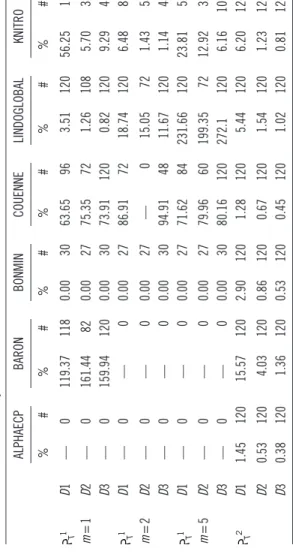
AlphaECP failed to obtain a solution in all experiment instances, whereas LINDOGlobal was able to obtain a solution in all experiment instances except for the demand distribution D2. However, for that pattern, it also resulted in a solution in the most number of instances.
Ta bl e 1 3. 1 Ov er all S um ma ry o f P er fo rm an ce M ea su re s ALPHAECP BARON BONMIN COUENNE LINDOGLOBAL KNITRO % # % # % # % # % # % # PT 1 D1 — 0 119.37 118 0.00 30 63.65 96 3.51 120 56.25 19 m = 1 D2 — 0 161.44 82 0.00 27 75.35 72 1.26 108 5.70 38 D3 — 0 159.94 120 0.00 30 73.91 120 0.82 120 9.29 45 PT 1 D1 — 0 — 0 0.00 27 86.91 72 18.74 120 6.48 87 m = 2 D2 — 0 — 0 0.00 27 — 0 15.05 72 1.43 53 D3 — 0 — 0 0.00 30 94.91 48 11.67 120 1.14 48 PT 1 D1 — 0 — 0 0.00 27 71.62 84 231.66 120 23.81 52 m = 5 D2 — 0 — 0 0.00 27 79.96 60 199.35 72 12.92 32 D3 — 0 — 0 0.00 30 80.16 120 272.1 120 6.16 106 PT 2 D1 1.45 120 15.57 120 2.90 120 1.28 120 5.44 120 6.20 120 D2 0.53 120 4.03 120 0.86 120 0.67 120 1.54 120 1.23 120 D3 0.38 120 1.36 120 0.53 120 0.45 120 1.02 120 0.81 120
Bonmin has low performance in obtaining a solution, but the qual-ity of the obtained solution is very good (optimal in many instances). Regardless of the number of inputs in the system, it was able to get a near-optimal solution for D1. The distribution D2 seems to present the most difficulty for given m and other parameters except for Bonmin.
For LINDOGlobal, the number of inputs in the problem setting has a negative impact on the quality of the obtained solutions. For other solvers, the behavior may not be monotone (e.g., KNITRO, Bonmin). However, in a very general qualitative sense, we get the impression that solver performance (in both criteria) tends to worsen as the number of inputs increases in the problem setting. This obser-vation has motivated us to construct the second formulation, PT2. For
PT2, the performances of all solvers have improved significantly in
terms of the number of instances for which a feasible solution was obtained; none of the solvers failed across the entire experimental bed. Also, the solution quality for all solvers except LINDOGlobal (for m = 1 case) has increased. These indicate that the formulation PT2
is more amenable to use on the available solvers. 13.3.2 ANOVA Assessment
The overall assessment presented earlier was based on the perfor-mances of the two formulations and the solvers in an aggregate sense. Next, we focus on the formulation PT2 and use the formal statistical
tool ANOVA to identify the factors that impact the solution quality significantly in a statistical sense.
We considered a three-way ANOVA where the factors are (1) K (representing the fixed replenishment cost) considered in four levels Ki, i = 1,…, 4; (2) W (representing the transportation cost coefficient, w)
considered in three levels, Wj, j = 1, 2, 3 as given earlier in the
experi-mental bed; and (3) the different solvers denoted by S with six levels,
Sk, k = 1,…,6 corresponding to the solvers in the order given earlier
with n = 10 replications (corresponding to the demand realizations) at each experimental instance. The response variables yijkl, i = 1,…,4; j =
1,2,3; k = 1,…,6; and l = 1,…,10 are taken as the percentage devia-tions of the soludevia-tions provided by the solvers from the optimal solu-tion, which is obtained by DP. The ANOVA study was conducted for each demand distribution separately.
The ANOVA tables for the three distributions are given in Tables 13.2 through 13.4. The performance statistics for each factor level computed across the other experiment parameters are tabulated in Table 13.5 for each demand distribution. Finally, the interaction effects of the factor levels are provided in Figures 13.1 through 13.3 for the each distribution, respectively. The inspection of these results reveals the following findings.
Firstly, all the factors and the interactions have significant impact on the solution quality, which is indicated by very large F values and correspondingly very small P-values, implying that the hypothesis that states that all factor levels have the same effect on the response variable is rejected for all three distributions. A closer inspection of the results provides further information regarding (1) the relative impact of the factors, (2) direction of the factor-level impact, and (3) the interaction effect. We treat each demand distribution separately.
Table 13.3 ANOVA for D2
SOURCE DF SEQ SS ADJ SS ADJ MS F P
K 3 640.025 640.025 213.342 754.86 0 W 2 542.101 542.101 271.051 959.05 0 S 5 1020.997 1020.997 204.199 722.52 0 K *W 6 1163.260 1163.26 193.877 685.99 0 K *S 15 134.743 134.743 8.983 31.78 0 W *S 10 120.064 120.064 12.006 42.48 0 K *W *S 30 347.503 347.503 11.583 40.99 0 Error 648 183.140 183.14 0.283 Total 719 4151.832
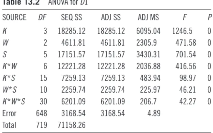
Table 13.2 ANOVA for D1
SOURCE DF SEQ SS ADJ SS ADJ MS F P
K 3 18285.12 18285.12 6095.04 1246.5 0 W 2 4611.81 4611.81 2305.9 471.58 0 S 5 17151.57 17151.57 3430.31 701.54 0 K *W 6 12221.28 12221.28 2036.88 416.56 0 K *S 15 7259.13 7259.13 483.94 98.97 0 W *S 10 2259.74 2259.74 225.97 46.21 0 K *W *S 30 6201.09 6201.09 206.7 42.27 0 Error 648 3168.54 3168.54 4.89 Total 719 71158.26
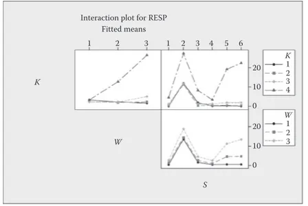
Consider Table 13.2. Comparing the F values, we observe that the most important factors are, respectively, K, S, W, and the two-way KW interaction. From Table 13.5, we see that K4, W3, and S2 (Solver Baron) result in the worst solution quality on average. Next, inspecting the impact of average effect of different levels of factors from Table 13.5, we see that the largest deviation from the optimal results is observed when fixed cost is highest at K4 level, when W is at the W3 level, and the solver S2 is used. From Figure 13.1, we observe that the differential effect as K increases depends on the level of W implying a significant interaction of K and W with the worst performance occurring at K4W3 combination. Although not as significant, there is also some interaction of K with the solvers. As K level changes from 3 to 4, the performance deteriorates sig-nificantly with solvers S5 (LINDOGlobal) and S6 (KNITRO). A similar relation also holds regarding the interaction between W and the solvers.
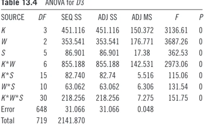
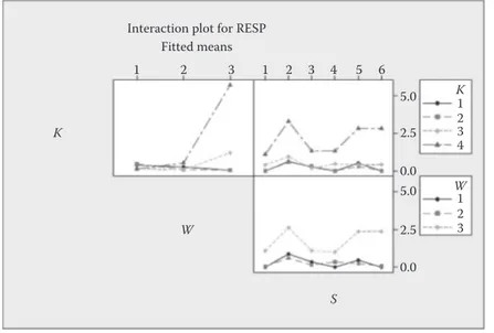
Similar analysis for D2 and D3 reveals the following. For D2, the factors with the highest F values are ordered as W, K, S, and the two-way interaction KW. Table 13.5 shows that there are less dras-tic differences between the average solution quality corresponding to different levels of the factors. Figure 13.2 shows that the KW inter-action is still significant, and the difference between the levels of K is highest for W3, where the interaction of solvers with K and W is reduced. The ordering of solver performances is similar to that of D1. For D3, we note that the factors with the highest F values are ordered as W, K, KW, and S. We again observe that the average solution qual-ity corresponding to different factor levels generally becomes closer
Table 13.4 ANOVA for D3
SOURCE DF SEQ SS ADJ SS ADJ MS F P
K 3 451.116 451.116 150.372 3136.61 0 W 2 353.541 353.541 176.771 3687.26 0 S 5 86.901 86.901 17.38 362.53 0 K *W 6 855.188 855.188 142.531 2973.06 0 K *S 15 82.740 82.74 5.516 115.06 0 W *S 10 63.062 63.062 6.306 131.54 0 K *W *S 30 218.256 218.256 7.275 151.75 0 Error 648 31.066 31.066 0.048 Total 719 2141.870
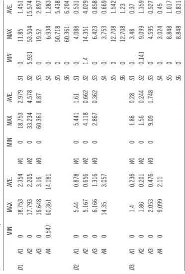
Ta bl e 13 .5 Re sp on se V ar ia ble S ta tis tic s f or D iff er en t F ac to rs MIN MAX AVE. MIN MAX AVE. MIN MAX AVE. D1 K1 0 18.753 2.354 W 1 0 18.753 2.979 S1 0 11.85 1.451 K2 0 17.793 2.205 W 2 0 33.234 4.578 S2 5.931 53.504 15.574 K3 0 16.648 3.16 W 3 0 60.361 8.87 S3 0 19.52 2.897 K4 0.547 60.361 14.181 S4 0 6.934 1.283 S5 0 50.718 5.438 S6 0 60.361 6.204 D2 K1 0 5.44 0.878 W 1 0 5.441 1.61 S1 0 4.088 0.531 K2 0 5.167 0.656 W 2 0 4.118 0.662 S2 1.4 14.351 4.029 K3 0 6.166 1.316 W 3 0 2.867 0.362 S3 0 6.423 0.858 K4 0 14.35 3.057 S4 0 3.753 0.669 S5 0 12.708 1.542 S6 0 12.708 1.23 D3 K1 0 1.4 0.236 W 1 0 1.86 0.28 S1 0 3.48 0.37 K2 0 1.86 0.201 W 2 0 1.56 0.244 S2 0.141 9.099 1.359 K3 0 2.053 0.476 W 3 0 9.09 1.748 S3 0 4.595 0.527 K4 0 9.099 2.11 S4 0 3.024 0.45 S5 0 8.848 1.017 S6 0 8.848 0.811
to each other, while the KW interaction is still emphasized and the interactions with the solvers become less emphasized.
From the earlier analysis, we see that the solvers’ performances get more and more closer to each other as the coefficient of variation of the demand distribution gets smaller and the worst performances
Interaction plot for RESP 1 K W S 1 2 3 4 5 6 8 K W 1 2 3 4 1 2 3 4 4 0 8 0 2 3 Fitted means
Figure 13.2 Factor interaction for D2.
Interaction plot for RESP 1 K W S 1 2 3 4 5 6 20 K W 1 2 3 4 1 2 3 20 10 10 0 0 2 3 Fitted means
are observed for the K4W3 large fixed cost and low transportation cost coefficient combination. Furthermore, S1, S3, and S4 (Solvers AlphaECP, Bonmin, and Couenne, respectively) are always among the best three performing solvers (although their ordering may change), whereas the worst performer is S2 in all three demand distributions. We observe that solver performances depend dras-tically on problem formulations as well as cost parameters. We should also mention that they may as well depend on possible user interventions such as initial point selections that were not imposed in our study.
Acknowledgment
The work of Ramez Kian is partially supported by TUBİTAK (The Scientific and Technological Research Council of Turkey).
References
Ballou, R.H. (2003). Business Logistics/Supply Chain Management, 5th edn. Prentice Hall, Upper Saddle River, NJ.
Berman, O. and Q., Wang. (2006). Inbound logistic planning: Minimizing transportation and inventory cost. Transportation Science 40(3): 287–299.
Interaction plot for RESP 1 K W S 1 2 3 4 5 6 5.0 K W 1 2 3 4 1 2 3 5.0 2.5 2.5 0.0 0.0 2 3 Fitted means
Chang, S. (1978). Production function and capacity utilization of the port of mobile. Maritime Policy and Management 5: 297–305.
Cheung, S.M.S. and T.L. Yip. (2011). Port city factors and port production: Analysis of Chinese ports. Transportation Journal 50(2): 162–175. Cobb, C.W. and P.H. Douglas. (1928). A theory of production. American
Economic Review 8(1): 139–165.
Coyle, J.J., C.J. Langley, B.J. Gibson, R.A. Novack, and E.J. Bardi. (2008).
Supply Chain Management: A Logistics Perspective, 8th edn. South-Western
College Publication, Cincinnati, OH.
Cullinane, K., T.-F. Wang, D.-W. Song, and P. Ji. (2006). The technical effi-ciency of container ports: Comparing data envelopment analysis and sto-chastic Frontier analysis. Transportation Research Part A 40(4): 354–374. Cullinane, K.P.B. (2002). The productivity and efficiency of ports and
termi-nals: Methods and applications. In C.T. Grammenos (Ed.), The Handbook
of Maritime Economics and Business, Informa Professional, London, U.K.,
pp. 803–831.
Cullinane, K.P.B. and D.-W. Song. (2003). A stochastic Frontier model of the productive efficiency of Korean container terminals. Applied Economics 35: 251–267.
Cullinane, K.P.B. and D.-W. Song. (2006). Estimating the relative effi-ciency of European container ports: A stochastic Frontier analysis. In K.P.B. Cullinane and W.K. Talley (Eds.), Port Economics, Research
in Transportation Economics, Vol. XVI. Elsevier, Amsterdam, the
Netherlands, pp. 85–115.
Cullinane, K.P.B., D.-W. Song, and R. Gray. (2002). A stochastic frontier model of the efficiency of major container terminals in Asia: Assessing the influence of administrative and ownership structures. Transportation
Research A: Policy and Practice 36: 743–762.
Dolan, E., R. Fourer, J.J. Mor, and T.S. Munson. (2002). Optimization on the NEOS server. SIAM News 35(6), 1–5.
Douglas, P.H. (1976). The Cobb–Douglas production function once again: Its history, its testing, and some new empirical values. Journal of Political
Economy 84(5): 903–916.
Estache, A., M. Gonzalez, and L. Trujillo. (2002). Efficiency gains from port reform and the potential for yardstick competition: Lessons from Mexico.
World Development 30(4): 545–560.
Gonzalez, M.M. and L. Trujillo. (2009). Efficiency measurement in the port industry: A survey of the empirical evidence. Journal of Transport
Economics and Policy 43(Part 2): 157–192.
Hatirli, S.A., B. Ozkan, and C. Fert. (2006). Energy inputs and crop yield relationship in greenhouse tomato production. Renewable Energy 31(4): 427–438.
Heathfield, D. and S. Wibe. (1987). An Introduction to Cost and Production
Functions. Humanities Press International, New Jersey, NJ.
Hwang, H.C. (2009). Inventory replenishment and inbound shipment sched-uling under a minimum replenishment policy. Transportation Science 43(2): 244–264.
Hwang, H.C. (2010). Economic lot-sizing for integrated production and transportation. Operations Research 58(2): 428–444.
Ingene, C.A. and R.F. Lusch. (1999). Estimation of a department store pro-duction function. International Journal of Physical Distribution & Logistics
Management 29(7/8): 453–464.
Jaruphongsa, W., S. Cetinkaya, and C.-Y. Lee. (2005). A dynamic lot siz-ing model with multi-mode replenishments: Polynomial algorithms for special cases with dual and multiple modes. IIE Transactions 37: 453–467.
Kian, R., Ü. Gürler, and E. Berk. (2014). The dynamic lot-sizing problem with convex economic production costs and setups. International Journal of
Production Economics 155: 361–379.
Kogan, K. and C.S. Tapiero. (2009). Optimal co-investment in supply chain infrastructure. European Journal of Operational Research 192(1): 265–276. Lederer, P.J. (1994). Competitive delivered pricing and production. Regional
Science and Urban Economics 24(2): 229–252.
Lee, C.-Y. (1989). A solution to the multiple set-up problem with dynamic demand. IIE Transactions 21: 266–270.
Lee, C.-Y., S. Cetinkaya, and W. Jaruphongsa. (2003). A dynamic model for inventory lot sizing and outbound shipment scheduling at a third-party warehouse. Operations Research 51(5): 735–747.
Lee, S.-D. and Y.-C. Fu. (2014). Joint production and delivery lot sizing for a make-to-order producer-buyer supply chain with transportation cost.
Transportation Research Part E 66: 23–35.
Lightfoot, A., G. Lubulwa, and A. Malarz. (2012). An analysis of container handling at Australian ports, 35th ATRF Conference 2012, Perth, Western Australia, Australia.
Lippman, S.A. (1969). Optimal inventory policy with multiple set-up costs.
Management Science 16: 118–138.
Notteboom, T.E., C. Coeck, and J. Van den Broeck. (2000). Measuring and explaining relative efficiency of container terminals by means of Bayesian stochastic Frontier models. International Journal of Maritime Economics 2(2): 83–106.
Pochet, Y. and L.A. Wolsey. (1993). Lot-sizing with constant batches: Formulations and valid inequalities. Mathematics of Operations Research 18(4): 767–785.
Rekers, R.A., D. Connell, and D.I. Ross. (1990). The development of a produc-tion funcproduc-tion for a container terminal in the port of Melbourne. Papers of
the Australiasian Transport Research Forum 15: 209–218.
Shadbegian, R.J. and W.B. Gray. (2005). Pollution abatement expenditures and plant level productivity: A production function approach. Ecological
Economics 54(2): 196–208.
Taaffe, E.J., H.L. Gauthier, and M.E. OKelly. (1996). Geography of
Transportation, 2nd edn. Prentice-Hall, Inc., Upper Saddle River, NJ.
Tongzon, J. and W. Heng. (2005). Port privatization, efficiency and competi-tiveness: Some empirical evidence from container ports (Terminals).
Tongzon, J.L. (1993). The Port of Melbourne Authority’s pricing policy: Its efficiency and distribution implications. Maritime Policy and Management 20(3): 197–203.
Tovar, B., S. Jara-Daz, and L. Trujillo. (2007). Econometric estimation of scale and scope economies within the Port Sector: A review. Maritime Policy &
Management 34(3): 203–223.
Trujillo, L. and S. Jara-Daz. (2003). Production and Cost Functions and their
Application to the Port Sector: A Literature Survey, Vol. 3123. World Bank
Publications, http://dx.doi.org/10.1596/1813-9450-3123.
Van Vyve, M. (2007). Algorithms for single-item lot-sizing problems with constant batch size. Mathematics of Operations Research 32: 594–613. Wagner, H.M. and T.M. Whitin. (1958). Dynamic version of the economic lot
size model. Management Science 5(1): 89–96.
Williams, M. (1979). Firm size and operating costs in urban bus transporta-tion. The Journal of Industrial Economics 28(2): 209–218.
Xu, S. (2013). Transport economies of scale and firm location. Mathematical