Final phase inventory management of spare parts under nonhomogeneous poisson demand rate

(1)

FINAL PHASE INVENTORY MANAGEMENT OF SPARE

PARTS UNDER NONHOMOGENEOUS POISSON DEMAND

RATE

A THESIS

SUBMITTED TO THE DEPARTMENT OF INDUSTRIAL ENGINEERING

AND THE GRADUATE SCHOOL OF ENGINEERING AND SCIENCE OF BILKENT UNIVERSITY

IN PARTIAL FULFILLMENT OF THE REQUIREMENTS FOR THE DEGREE OF

MASTER OF SCIENCE

by

Sertalp Bilal Çay

June 2013

(2)

ii

I certify that I have read this thesis and that in my opinion it is full adequate, in scope and in quality, as a dissertation for the degree of Master of Science.

___________________________________ Prof. Nesim Erkip (Advisor)

___________________________________ Asst. Prof. Zeynep Pelin Bayındır

______________________________________ Asst. Prof. İsmail Serdar Bakal

Approved for the Graduate School of Engineering and Science

____________________________________ Prof. Levent Onural

(3)

iii

ABSTRACT

FINAL PHASE INVENTORY MANAGEMENT OF SPARE PARTS UNDER NONHOMOGENEOUS POISSON DEMAND RATE

Sertalp Bilal Çay M.S. in Industrial Engineering Supervisor: Prof. Nesim Erkip

June 2013

In product lifecycle, there are three phases, initial phase, normal phase and final phase. Final phase begins when the product is out of production, and ends when the last contract expires. It is generally the longest period in the lifecycle. Although the product is not manufactured any more, spare parts of the product need to be supplied to the market. Firms need to provide these parts at the retailer level until the end of the phase due to legal responsibilities. Because of lack of historical data and unavailability of forecasting, retailers need a systematic policy to decide replenishment quantity and time to prevent excessive holding, backordering, unit and setup costs. In our problem, we assume that demand of the spare part is a non-homogeneous Poisson process where the rate parameter is a non-increasing function of time. We consider all costs and lead time are fixed and known. Due to characteristics of the final phase, the planning horizon is taken as finite and known.

In this study, we developed two alternative heuristics for retailer’s problem to minimize total cost during the final phase. First heuristic is a continuous-review policy based on estimation of future replenishments by solving series of deterministic demand sub-problems. Second heuristic is a periodic-review policy with variable period lengths, which solves myopic problems, by selecting subsequent time points to check inventory

(4)

iv

position. We also developed a simulation model to evaluate performances of the heuristics.

This study provides an efficient way to decide on replenishment quantity and time. Limited numerical results show that heuristics provide near-optimal results for homogeneous cases studied in the literature. Moreover, this is one of the initial studies that considers final phase with non-homogeneous demand rate. In that sense, it makes a contribution to the literature of final phase problems and provides a systematic way of replenishment decisions for the retailers.

(5)

v

ÖZET

HOMOJEN OLMAYAN POISSON TALEP DAĞILIMLI YEDEK PARÇALARIN SON AŞAMADA ENVANTER YÖNETİMİ

Sertalp Bilal Çay

Endüstri Mühendisliği Yüksek Lisans Tez Yöneticisi: Prof. Dr. Nesim Erkip

Haziran 2013

Bir ürünün yaşam döngüsü üç aşamadan oluşmaktadır; ilk aşama, normal aşama ve son aşama. Son aşama, ürünün üretimden kaldırıldığı anda başlayıp, son müşteri sözleşmesi bitene kadar devam eder. Genel olarak bu süreç ürünün yaşam döngüsündeki en uzun aşamadır. Bu aşamada ürün üretilmemesine karşın yedek parçaları sağlanmaya devam edilmelidir. Bu yedek parçalar perakendeci seviyesinde, yasal zorunluluklar bitene kadar tutulmalıdır. Talep geçmişi ve tahminin yapılamamasından ötürü doğabilecek aşırı bekletme, ısmarlama, ürün ve sipariş maliyetlerini engellemek için perakendeciler sistematik bir yaklaşıma ihtiyaç duymaktadır. Bu problemde, talebin homojen olmayan Poisson dağılımla geldiği ve talep kurunun artış göstermeyen zamana bağlı bir fonksiyon olduğu varsayılmıştır. Problemdeki tüm maliyet parametrelerinin sabit ve bilindiği varsayımı altında sınırlı bir zaman aralığı için çözüm geliştirilmiştir.

Bu çalışmada, perakendecinin problemini çözmek için iki adet sezgisel yaklaşım geliştirilmiştir. İlk yaklaşım bir sürekli envanter yöntemi olup, gelecek zamana ait talebin değerlendirmesine ve bir dizi deterministik probleminin çözümüne dayanmaktadır. İkinci yaklaşım bir aralıklı envanter yöntemi olup, aralık uzunluğu miyop olarak çözülen küçük problemlerin sonucuna göre değişiklik göstermektedir. Geliştirmil olduğumuz bir simülasyon aracıyla bu çözümler test edilmiştir.

(6)

vi

Bu çalışma, perakendecinin sipariş zamanı ve büyüklüğü konusunda etkili bir çözüm önermektedir. Yapmış olduğumuz sınırlı sayıdaki sayısal sonuçlara göre homojen talep dağılımı için optimal çözüme yakın sonuçlar vermektedir. Ayrıca bu çalışma, son aşamada homojen olmayan talep dağılımını kullanan ilk çalışmalardan biridir. Bu açıdan son aşama problemleri literatürüne bir katkıda bulunup, perakendeciler için sistematik bir sipariş yönetimi önermiştir.

(7)

vii

ACKNOWLEDGEMENT

I would like to offer my sincerest gratitude to my advisor, Prof. Nesim K. Erkip, who has guided and supported me with his patience, motivation and vast knowledge. He provided many insightful ideas and discussions about the problem. I am deeply grateful to my committee, Asst. Prof. Zeynep Pelin Bayındır and Asst. Prof. İsmail Serdar Bakal for their helpful suggestions and hard questions which illuminated me.

I am thankful to my former research advisor during my undergraduate, Assoc. Prof. Murat Fadıloğlu for being with me during my first steps to research world. I owe a very important debt to Prof. Barbaros Tansel for his effect on my research career. I will always remember him. I also would like to thank all staff and faculty members of Industrial Engineering Department for their support.

Without support of Emre Haliloğlu, Enes Bilgin, Emre Kara and Hüseyin Duman, earning an MS degree would be difficult and challenging. Thank you all for your valuable friendship, which makes this time period special.

I owe a lot to my parents, Mustafa Çay and Fatma Çay, my in-laws H. Barış Diren and Ceyla Diren and my sister Mehtap Hilal Çabuk for their endless love and support. They presented their help in every stage of my master and this thesis.

Most importantly, my heartfelt and deepest gratitude and thanks go to my dear wife, Pelin Çay, for her endless love, motivation, support, encouragement and patience. It is a blessing to finish my master with you. You are my guiding light in my life.

I am grateful to TÜBİTAK-BİDEB for awarding me with their graduate scholarship 2210. Their support always motivated me to focus on my research.

(8)

viii

LIST OF FIGURES

Figure 2.1 Planning horizon of the problem ... 8

Figure 3.1 Relation between replenishment quantity decision and its effects. ... 28

Figure 3.2 Behavior of Reorder Level during Final Phase when Demand Rate is Non-Increasing Function of Time ... 35

Figure 3.3 Order Statistics of Arrival Times of Demands ... 38

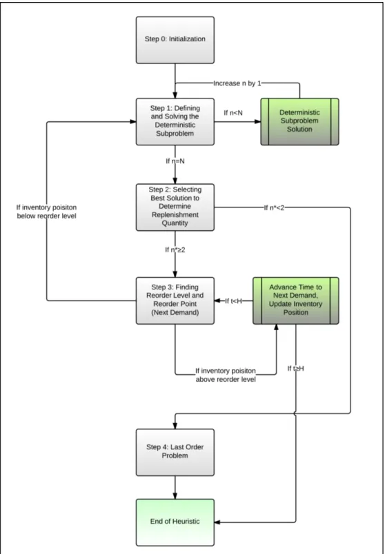
Figure 3.4 Flow chart of the 1st Heuristic ... 41

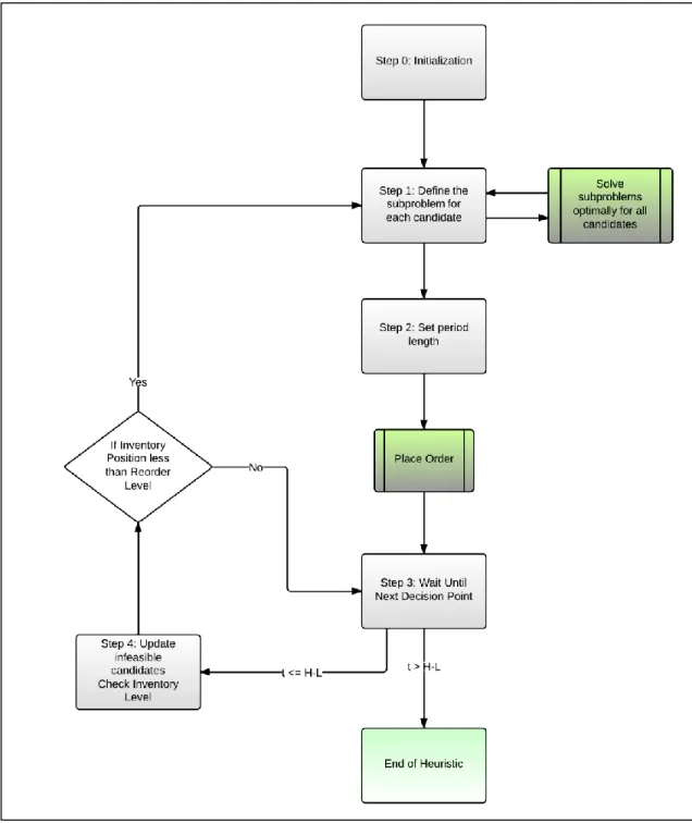
Figure 3.5 Steps of the 2nd heuristic ... 46

Figure 3.6 Effect of constant demand rate on reorder level ... 51

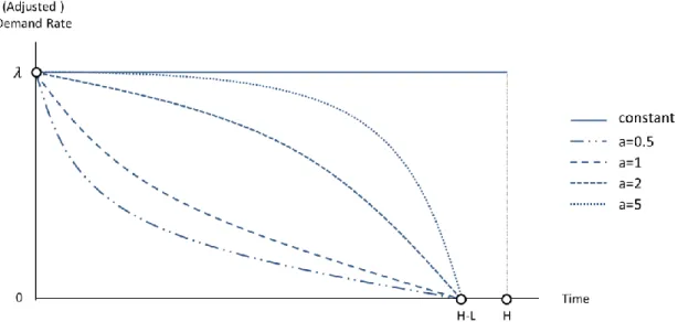
Figure 3.7 Behavior of Adjusted Demand Rates for Various Selection of the Parameter ... 52

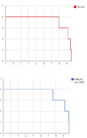
Figure 3.8 Order-up-to level by THM for Teunter and Haneveld’s problem ... 54

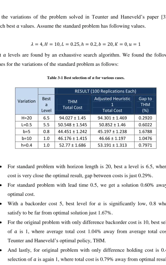
Figure 3.9 Order-up-to level by First Heuristic for Homogeneous Case ... 54

Figure 3.10 Side by side comparison of THM and First Policy’s Order-Up-To Level with Adjusted Demand Rate ... 55

Figure 4.1 User Interface of Insys Simulation Tool ... 66

Figure 4.2 Insys is simulating a case, where demand rate is a decreasing linear function of time. ... 67

Figure 4.3 A sample output file of Insys. ... 68

Figure 4.4 Inventory Position-Level vs. Time Graph for Standard Problem by using 1st Heuristic (Appendix 3) ... 69

(10)

x

LIST OF TABLES

Table 3-1 Best selection of for various cases. ... 57

Table 3-2 Best selection of adjustment parameter ... 58

Table 3-3 Regression Results for Power Approximation ... 59

Table 3-4 Comparison of Best and Approximated Adjustment Parameter... 61

Table 4-1 Setups for Problem Parameters ... 71

Table 4-2 Comparison of Simulation Results for 1st Heuristic Different Setups, ... 72

Table 4-3 Comparison of Simulation Results for 1st Heuristic Different Setups, ... 72

Table 4-4 Comparison of THM and 1st Heuristic with Different Adjustment Parameter on Standard Problem ... 73

Table 4-5 Comparison of THM and 1st Heuristic with Different Adjustment Parameter for ... 74

Table 4-6 Effect of Adjustment on Different Setup Cost Settings ... 75

Table 4-7 Change in Total Cost for Different Demand Rates ... 76

Table 4-8 Comparison of THM, 1st and 2nd Heuristics for Standard Problem ... 76

Table 4-9 Comparison of 1st and 2nd Heuristics for on Standard Problem ... 77

(11)

1

Chapter 1

Introduction

In manufacturing and logistics, spare part management (SPM) is an important component to achieve desired service level at minimum cost. Besides their usage for repairing, spare parts can also be used to replace failed components, thus extending lifetime of the products. Decision in SPM includes different aspects from forecasting to inspection. Due to its large range of decisions, in industry more than 50% of the maintenance costs are due to spare parts. Moreover in some sectors more than half of the down times are due to unavailability of adequate spare parts [24]. In 2011 press release, Technology Services Industry Association (TSIA) stated that average value of spare parts inventory is 17% of total service revenue and spare parts are critical to delivering prompt quality service [29]. Obviously, SPM is a vital factor for success in manufacturing and business today.

(12)

2

Spare part management consists of different phases throughout the production process. In each phase, supply and demand structure changes and often these phases are studied separately. A major one of these life periods is called Final Phase, which is also known as End-of-life (EOL) phase in the spare part management literature. This phase starts when the product is out of production line and continues until last costumer contract or warranty expires. In this phase, although part is no longer manufactured, the service requirements still continue, hence the spare parts should be supplied until the end. There are also some legal stipulates to firms to provide spare parts until last customer contract expires. Therefore, unavailability of sufficient spare parts inventory can lead some penalty costs which could be more than product value (due to replacement). On the other hand, excessive inventory can lead huge disposal costs at the end of the final phase. Final Phase is known to be the longest period in a product life-cycle in general [32]. For instance in European Union every goods need to have two-years of guarantee at minimum [9]. Moreover, based on Supply of Goods and Services Act 1982, spare parts for motor companies should be provided at least for 10 years [24]. These instances prove that inventory control of spare parts during final phase is a vital decision for enterprises. Spare parts can be stored in different levels in a multi-echelon inventory system. Based on the industry, parts may be needed to be available at retailer level to provide fast response and lower backordering cost. Especially if production of spare parts is costly for the company, they may want to produce spare parts in large batches, as in the case of serial production. Therefore, retailers need to order spare parts to keep their inventory at a reasonable level.

As described above, this thesis focuses on retailer-level inventory management of spare parts during final phase. This problem is originally discussed through a forecasting-based approach by Moore [19] in 1971, where they define all-time requirements of consumable spare parts for motor-car industry. In his thesis, Pourakbar [21] provides a comprehensive analysis on problem, discussing different approaches.

(13)

3

This study evaluates problem on retailer’s behalf. Therefore, our objective is minimizing total cost of the retailer in a decentralized system. The total cost is consisting of unit, setup, holding, and backorder costs. Since we study on a decentralized system, retailer need to decide own replenishment times and quantities, which are our decision variables. Since inventory management varies much based on product type, industry type and other conditions, we decided to focus on the following setting:

 Time horizon is finite and known. This is a common setting in final phase studies because expiration of last contract is known beforehand. Time is considered as a continuous variable over planning horizon.

 At the end of the planning horizon, all backordered demands should be satisfied with a single last order. This one is a part of legal requirements.

On top of this setting, we made the following assumptions to work on a clearer problem:  Unit, setup, holding and backorder costs are constant and known at time zero.  Lead time is constant and known.

 Unit demands are unit-sized.

 Demand is a Non-Homogeneous Poisson Process with a non-increasing demand rate over time.

In this study we proposed two heuristics from different perspectives to solve the retailers’ inventory management problem.

Following sections in this thesis as follows; in second chapter, problem definition and literature review about spare parts inventory management and final phase is given. In

(14)

4

third chapter, our proposed solution methodology is presented. Paper follows with computations in fourth chapter and conclusion in fifth chapter.

(15)

5

Chapter 2

Problem Definition and Literature

Review

2.1. Problem Definition

Spare part management consists of different echelon levels in general. Each level requires strategic, tactical and operational decisions. These decisions could be made either by a single decision maker or each level may have its own. In this thesis, we focused on a decentralized system with a focus on single retailer. Problem is based on retailer’s controlling spare part inventory in the final phase. As stated before, retailer is the only decision maker and so the purpose of this study is minimizing its total cost in a finite horizon.

(16)

6

In management of the spare part inventory, retailer faces with some challenges. One of the biggest challenges in this management is unavailability of data for forecasting the future demand. This is generally the case in the final phase. Since retailer has limited or inadequate data for forecasting and demand is unknown, retailer should estimate the future demand which makes inventory management much more difficult. On top of that, a certain customer service level may be desired for either cost minimization or customer satisfaction. Service level is especially vital in case of non-zero lead time. Little tardiness in replenishment decision time may lead unexpected high costs for the retailer. Yet another vital decision appears on replenishment quantity. Underestimation of the future demand leads smaller replenishment quantities which may increase the total number of the setups, thus total setup costs. On the other hand overestimation of the demand may lead higher holding costs and moreover, excess inventory could be available at the end of the final phase.

In this thesis, we defined the retailer’s problem with the following assumptions;

 Planning horizon is finite and known. This assumption is based on the fact that expiration of the last customer contract and legal responsibilities are known by the retailer.

 Unit, setup, holding and backorder cost parameters are fixed and known.

 Lead time for the supplier is fixed and known. Lead time is independent from replenishment quantity and time. Thus we assume supplier does not spend time for production; there is always adequate inventory at supplier level.

 Demand is a Non-Homogeneous Poisson process with a time-dependent rate. This rate is assumed to be a non-increasing function of time. In some cases, we also assume that rate of the NHPP reaches zero at the end of the planning horizon.

(17)

7  All demands are unit-sized.

 Backordering is allowed. Demands are met whenever inventory is available.  If horizon ends with some backorders, a last order is given to meet all

backordered demands.

 There is no salvage cost at the end of the horizon. Therefore, if inventory position is positive at the end of the horizon, all items are disposed.

In this thesis we focused on a retailer’s problem within a single echelon system and there is single type of product. Hence our objective is minimizing total cost of the retailer. Before going into details, we know that retailer has two different extreme solutions. First extreme solution is backordering all demand during final phase and meets all these orders at the end of horizon. Second extreme solution is placing a huge replenishment order at the beginning of the phase.

Assume that retailer applies the first extreme solution and backorders all the demand during time horizon. Due to legal responsibilities, he needs to meet all these demands in a single order and he pays backordering (penalty) costs. If penalty cost is sufficiently small, this extreme solution could be the best choice for the retailer. Otherwise, systematic planning of the replenishments may balance the holding, setup and backordering costs.

There are two decisions need to be taken by the retailer. First one of these decisions is “When I need to place a replenishment order?” Second question is “How much I need to order for each replenishment order?” Correct answers to these two decisions are affected by total cost components: setup, unit, holding and backorder costs. Moreover, these questions needed to be answered throughout the horizon. So our policies should be capable of answering these questions at any time during the horizon.

(18)

8

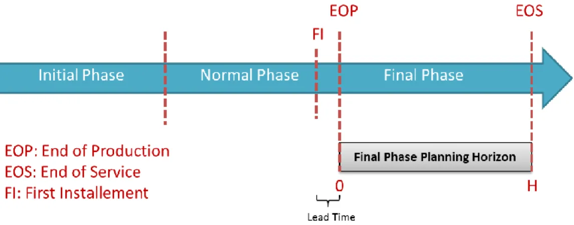
Due to nature of the final phase, our planning horizon is the time between End of Production (EOP) and End of Service (EOS) where last customer contract expires. In this thesis, the problem starts just before EOP to start horizon with a sufficiently large inventory. Therefore both heuristics starts at First Installment (FI) point, which is lead time length before EOP.

Figure 2.1 Planning horizon of the problem

In order to find satisfying answers to retailer’s problem we developed two heuristics. These heuristics answers these questions in a systematic way for the retailer. We detailed these heuristics in the Chapter 3.

2.2. Literature Review

The problem considered in this thesis can be classified under different stream of literature of inventory management, such as Spare Part, Obsolescence, Product Life-Cycle and Final Phase. In this subsection, there are numerous studies that are related with more than one topic among these streams. We try to show the importance of this study in these streams while defining the problems and classifying previous studies, in given order.

(19)

9 Spare Part Management

Spare Part Inventory Management (SPIM) is a broad topic that includes various aspects. The more relevant studies in SPIM are conducted by Fortuin [11, 10] in 1980 and 1981, which define all-time requirements (final order) of spare part inventories. He studies on management of spare parts of a product that have risk of failure, such as electronic products, for the “service after sales” department. He defines the product life-cycle consist of three phases. There are initial, repeat and the final phases. He assumes exponentially decreasing demand in his study.

Another relevant study in SPIM literature is presented by Geurts and Moonen [13] in 1992. In their paper, they analyze and present how ‘insurance type’ spare parts are needed to be keep. They use Dynamic Programming (Markov Programming) approach in this paper, which is also supported by numerical examples. While deciding on uncertainty parameters, they also utilize their approach to measure how good the decision strategy is.

Obsolescence

The main stream of our thesis, Final Phase studies are also related with finite horizon inventory problems with obsolescence. Hadley and Whitin [14] provides the classical obsolescence problem in 1963. In this study demand is a random variable and occurs in time periods independently. Obsolescence time is known or a finite number of possible obsolescence times are given with their respective probabilities. They solve this problem with a dynamic programming approach.

In 1997, David et al. [5] provides the continuous version of the classical obsolescence problem defined by Hadley Whitin. They provide a dynamic programming model for the finite horizon problem, where demand rate is fixed while lifetime of the items follows a known random distribution. In this problem, they observe that there must be a time

(20)

10

where ordering to the end is the optimal option. This corresponds to “last-order problem” in our heuristic. This study is also provides structural properties of the problem.

Life Cycle

Elements such as demand direction, length of horizon and stochasticity of the parameters lead different problem definitions in inventory studies. Hence, even for the very same product, we need to apply different inventory policies for the different phases during its life cycle. Often, inventory studies encapsulate a certain time interval in the product life. Such as, our heuristics described in this thesis are useful for a specific time interval in the product life-cycle due to its features and assumptions. There are numerous studies that emphasize these differences. For instance, Solomon et al. [27] showed the life-cycle phases and their distinct features of electronic equipment. They divided electronic product’s life-cycle in six phases. There are defined as introduction, growth, maturity, decline, phase-out and obsolescence phases. In this study, they mention on last-buy decision in the obsolescence phase, which is relevant to time-period we interest in this thesis and it will be discussed later in detail. One of the earliest studies that focus on the time interval we interest is performed by Cohen and Whang [4] in 1997. Similar to our study, they focus on the service after sales operations. On top of the management of spare parts, they consider an independent service operator which leads competition. Hence they used a ‘game-theoretic’ approach in their study. Their decision variables are completely different from ours, they decide product price, after-sales service quality and after-sales price in their problem.

Another interesting research that focuses on product life-cycle is performed by Bradley and Guerrero [2] in 2008. This paper focuses on product design to a better utilization of life-cycle mismatch of the components in a product. In this paper, one of the alternatives that are used to manage life-cycle mismatch is called “life-time buy” or “last-time buy”

(21)

11

which corresponds the final decision of inventory operations. This is exactly the same topic that we cover in this thesis.

Another study of Bradley and Guerrero [1] published in 2009 deals with lifetime buy (last-time buy) decision for multiple obsolete parts. Lifetime buy policy is argued to be the necessary when product life-cycle mismatch occurs on spare parts of a product. They prove the existence and the uniqueness of the solution to the problem, however since the solution cannot be expressed in closed-form, they suggest two heuristics which gives upper and lower bounds on the solution. They show results for stationary and non-stationary demand, and suggest that the heuristics give accurate results for the non-stationary demand case.

In their 2011 paper, Dekker et al. [6] inspect the various aspects of life-cycle phases of spare part management. They mention about unique and difficult cases on managing the spare part inventory and focus on forecasting strategies. Life-cycle phases mentioned above are also available in this study, while they give an importance on the life-cycle of spare part demand. Interested readers may look for the case studies in Fokker Services, IBM, IHC Merwede and Voestalpine Railpro companies, presented in this paper.

Spengler and Schröter [28] developed tools for information management on a closed-loop supply chain at the End-of-Life service period. They model the management of production and recovery system of spare parts and emphasize the importance of several strategies. This study is important since it combines end-of-life service period with product design with a different view. In their paper, they show the difficulties to manage spare part inventory during end-of-life service period. It is known that final phase lasts for many years for electronic equipment [30]. These are the loss of economies of scale since the product is no longer manufactured, possible differences between product generations (hence spare parts may differ), limited flexibility of the spare parts and

(22)

12

possible problems on providing materials for spare parts. On a case study, they provide the output of their “system-dynamics” model for spare parts.

Final Phase

Now, we will focus on more relevant studies to our work which focus on spare part inventory management in the final phase. Final phase is also called with different definitions such as “end-of-life service”, “post-product life” and “after-sales service period”. The problem considers the inventory in the Final Phase period is also known as Life Inventory Problem” (EOL), “Final Buy Problem” (FBP) and the “End-of-Production Problem” (EOP) [23]. In this part we will review these relevant studies and emphasize the similarities and differences of our work with them. Note that the terms describing final phase are used interchangeably.

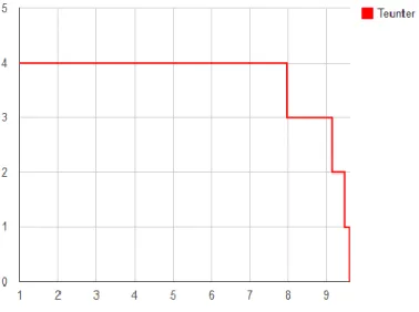
In their paper dated 1998, Teunter and Haneveld [33] described the final order problem. They solve the problem of “last-order” for the client, who will give a final order of spare parts from manufacturer due to discontinuity of spare part supply of the manufacturer. Client is assumed to have a machine which needs these critical spare parts to operate. Client wants to use this machine at least for a certain amount of time. Therefore, client should keep a sufficient inventory of these critical spare parts. They suggest an order-up-to level policy for this last order quantity. They found it by minimizing the order-up-total discounted cost. On 3 different examples they show that their model provides near-optimal results. There are some features of their problem, which is significantly different from the problem considered in this thesis. Teunter and Haneveld consider the time-period where service agreement ends, while we consider time between End-of-Production and End-of-Service (Final Phase) period. Moreover, they solve this problem for only one final order, while we allow replenishments during the time horizon which leads different assumptions.

(23)

13

In another study of Teunter and Fortuin [30], they study on the same problem with supplier’s perspective. In this case the decision maker is the service department of the supplier. However, the ordering structure is the same as Teunter and Haneveld’s study: only one last order is allowed to make for decision maker [33]. For given cost parameters, they reach near to optimal solutions of the quantity of the last order. They both provide ‘optimal’ final order by using stochastic dynamic programming and a ‘near-optimal’ final order level by using an explicit cost formulation. They show that the explicitly defined final order level is near to optimal final order level, which is practical to compute. Moreover, in this study they suggest a “remove-down-to” level, where they defined discrete time intervals and remove some spare parts from the stock if the inventory level is above the “remove-down-to” level. This study is important, because they take decisions after final phase started due to “remove policy”. Although they only remove items from the stock instead of replenish it as we cover in this thesis, this paper is closely related with ours since they allow actions during the time horizon.

In their 1999 paper, Fortuin and Martin [12] define phases of the spare part life-cycle. It’s one of the earliest study that use term “final phase” by referencing Teunter and Fortuin’s definition of End-of-Life service (EOL) [31]. This is a comprehensive study that shows different aspects of management of spare part inventory. It covers logistics, demand and delivery, management concepts of spare parts and also devotes a section to show differences between spare part inventory management with traditional approaches. They emphasize the distinction between phases of the spare part life-cycle, which are defined as initial, normal and final phase. In the following paragraphs, we will also review the work of Teunter and Haneveld [32] in 2002, which use the same final phase definition as in this paper.

Cattani and Souza [3] consider the effect of delaying the end of life buy in their 2002 paper. Their study is slightly different from Teunter and Haneveld’s research in terms of time of the final order (end-of-life buy) [33]. By using the information obtained by

(24)

14

delaying the final order decision, they argue that the underage and overage costs can be reduced. For different settings they show that the cost benefit of delaying the decision is non-decreasing function of time and concave. This is a remarkable result for the manufacturers who can delay their final order decision. They used the newsvendor problem as a basis to calculate costs of initial problem. On numerical experiments they provide how effective their model is.

Draper and Suanet’s work in 2005 includes various and detailed information about IBM’s inventory operations [7]. They stated that IBM divided inventory life-cycle into three phases: Early-Life, Mid-Life and End-of-Life. Their definition of End-of-Life phase is precisely the same as we define final phase. They note that this phase takes 7 years on average, although it varies a lot for different PC parts. They also stated that Service Parts Logistics organization is responsible for the actions in the end-of-life phase and used a ‘last-order’ at the beginning of this phase. This is precisely the problem that we mentioned above. They indicate that specialized algorithms are being used for this decision where historical data and demand forecast play a significant role. They refer the paper of Teunter and Haneveld for more information on last-buy problem [32]. Inderfurth and Mukherjee [17] consider different approaches in the final phase in their paper dated 2008. They differentiate the different phases of the product life-cycle similar to studies mentioned above. They stated that the managing the spare part inventory between end-of-production (EOP) to end-of-service (EOS) is especially challenging for many industries. This time period corresponds to final phase (or post-product life cycle) in our study. Assumptions and observations in this paper are very close to our problem. They show how the problem can be modeled as a Decision Tree and can be solved by Stochastic Dynamic Programming procedure. Moreover, they propose a relatively simpler heuristic by inspired by the solution of the dynamic programming.

(25)

15

Another study on the spare parts inventory management in the final phase is conducted by van Kooten and Tan [34] on parts under condemnation. Their model includes repairs of the spare parts. They suggest a continuous-time transient Markovian Model with certain repair probability and repair lead time.

Pinçe and Dekker [20] deal with the inventory of slow moving items subject to obsolescence in their paper dated 2011. They consider a continuous review inventory system and works in a similar environment to this problem. They assume that the demand rate drops a lower rate in a known time during the horizon. In this study, policy changing is proposed and an approximate solution of time to shift to new control policy is given. Advantages of such a shift are also described in the paper. During all horizon demand is assumed to follow Poisson Process with a constant rate, which drops to another constant rate at a known time. In that sense, their demand definition is one of the studies that are close to our problem. The policy used in the paper is one-for-one replenishment policy for both policies (initial policy and new policy) with different parameters. Our problem is slightly different from their definition and includes setup cost, which makes one-for-one replenishment policy an undesired alternative. For the problem they consider, they achieve satisfying numerical results that show the superiority of the switching.

There are also some studies that cover the different aspects of the final phase problem. Pourakbar et al. [23] suggests alternative decisions in the final phase such as offering a new product. They discuss the effects of such alternatives and show how they are more cost-efficient than keeping spare parts inventory at some point in the final phase. Hence, their study examines the cost trade-offs of such policies and give an exact expression represents expected total cost. They also show that such an expression leads the solution of last-order quantity and time to switch policies simultaneously. Their study is based on a real-life study of a major consumer electronic goods manufacturer, which is common in final phase studies. They developed two models, first, an alternative service policy

(26)

16

and second, a more sophisticated model for the cost function which is closer to real-life cases. In the study, demand is assumed to follow non-stationary Poisson process, which is also an assumption in this thesis. Moreover, horizon is finite and cost parameters are fixed and known similar to ours. However, they consider only “one-time buy” policies with review and scrapping options. Since we allow multiple orders during the final phase and associate a setup cost for this operation, the total cost structure and the behavior of the solutions to the problems are different from each other, respectively. In 2012, Pourakbar and Dekker [22] combine customer differentiation with the final phase inventory problem. Note that their study is different from other studies in the final phase literature, where procurement (replenishment) is an available option as we assume and they also use non-stationary demand rate. They show that their model reaches remarkable cost improvements on the problem.

Now, we will cover two researches that are very close to our problem, in detail.

In the study of Inderfurth and Kleber [16] in 2013, alternative management of spare part inventory in End-of-Production phase is studied. Due to challenges in managing the spare part inventory at this phase, they argue that options such as extra production and remanufacturing provide flexibility to the manufacturer. For this problem, they provide order-up-to levels for extra production and remanufacturing options, very similar to our model in this thesis. The decisions are told to be simple compared the complexity of the problem. They show that the problem can be modeled as a stochastic dynamic optimization problem. However, the policy to minimize average total cost is found to be too complex. Therefore, they suggest simple order-up-to policies, which are shown to be worked well for most of the cases when policy parameters are chosen appropriately. Their research is a great contribution to the literature, considering the number of studies about the final phase that considers extra production.

(27)

17

Note that, our study has similarities to the problem they worked. First of all, in both studies the time horizon is defined as the final phase (end-of-production phase) and assumed to be finite and known. Second, cost parameters are assumed to be fixed and known. Third, demand is assumed to be stochastic. Fourth, extra production is possible with a major setup cost. And lastly, the objective is to minimize total cost. Although the working environment is defined very similar, our approaches differentiate in the modeling phase. First of all, they discretize the time intervals into periods; hence their model suggests a periodic review policy. As we will see in following sections, our heuristics are continuous-review policies, indeed. Second, they update the estimation of the demand along the horizon while we assume that the distribution of the demand is known due to historical data beforehand. Third, their application area is automotive sector; hence they benefit from easiness of remanufacturing which does not take major setup time and setup cost. Our study focus on general cases hence remanufacturing is not an option. Lastly, they stated that extra production is only available with a minimum order quantity. We allow extra production for any quantity during the final phase. The other research that is close to our work in the literature is conducted by Teunter and Haneveld [32] in 2002. Actually our study is inspired by the problem they defined in their paper. Hence, we will extensively cover the details of this study in here and describe the similarities and differences with ours. We also used this study as a benchmark in our numerical experiments.

They study on manufacturer’s spare part inventory problem in the final phase. Since the expiration of last contract is known, they assume that the planning horizon is finite and known. There is no setup cost in the study; hence the replenishments are unit sized. Note that, they allow replenishments after the beginning of the final phase, but with a higher price. Demand is assumed to be stationary Poisson process. They propose an initial order-up-to level for the initial order, which is also known as the “last-order”, “final buy” and “lifetime buy” in the literature, and then provide order-up-to levels for the

(28)

18

remaining horizon. Since there is no setup cost, it is an ( ) inventory policy, where “S-1” is considered as a reorder level. Manufacturer should place unit-sized replenishment orders whenever the inventory position drops below the order-up-to level of the current time. They solved this problem optimally and provide a method which gives (1) initial order quantity and (2) time period length where order-up-to level is constant. By using this information, one can calculate the order-up-to level for any given time.

The problem we consider shows similarities to theirs in the following aspects. (1) The planning horizon is finite and known. (2) The cost parameters are known and fixed (holding, backorder). (3) Replenishments are allowed during the final phase. (4) Demand follows Poisson process. (5) A reorder level-order up to level policy is suggested.

We can also list the different aspects of our solution method as follows. (1) Setup cost exists and fixed. (2) Lead time is non-zero and fixed. (3) Poisson demand rate can be defined as non-stationary. (4) Unit cost is fixed and same during planning horizon. Note that among they suggest (1) and (3) as an extension to their model. In our problem, we assume that demand of the spare part is a nonhomogeneous Poisson process where the rate parameter is a non-increasing function of time.

In this study, we developed two heuristics for retailer’s problem to minimize total cost during the final phase. One of these heuristics is a continuous-review policy while the second one is a periodic-review policy. Due to complexity of the problem, we provide near-optimal results with these heuristics. This is one of the initial studies that considers final phase with non-homogeneous demand rate with replenishment option. In that sense, it makes a contribution to the literature of final phase problems and provides a systematic way of replenishment decisions for the retailers.

(29)

19

Chapter 3

Solution Methods

To solve a finite horizon problem, there are two types of policies based on the time of the decision. First type of approach is providing a static policy, where the problem is solved at the beginning of the horizon and applied thoroughly. For instance, in their paper, Teunter and Haneveld find the optimal order-up-to levels before the time horizon is started and these decisions are applied throughout the horizon [32]. All orders are given based on these optimal order-up-to levels. Second approach is constructing a rolling policy, where the decisions are given in continuous time. Such rolling policies are usually applied when the system changes over time. An order-up-to level can be used if applicable.

This problem, due to its very nature, is hard to solve optimally. Scarf showed that finite horizon problems can be solved with an optimal ( ) inventory policy by using

(30)

20

dynamic programming [25]. To the best of author’s knowledge, there is no optimal solution to our problem in the literature.

In this study, two heuristics are provided to solve retailer’s problem. Both of these heuristics are rolling policies with an approximation to the unknown optimal solution. There are two decisions variables in this problem, reorder level and order-up to level. Both policies use same reorder level mechanism however their selection of order-up-to level varies.

Our first heuristics provides a continuous review policy with look-ahead capability into remaining time horizon. Replenishment decisions are independent from past decisions and affected by the residual time. For each decision, a deterministic subproblem, between current time and end of horizon, is solved to estimate future orders. Solution to the deterministic subproblem is obtained by using Johnson and Montgomery’s notes on the “Continuous Review Lot Size Problem” [18]. Deterministic subproblems will be explained in detail in section 3.2.2. This estimation helps us to decide on replenishment quantity because when the number of remaining orders is known (or fixed), then the deterministic demand subproblem problem can be solved optimally (Lot Size Problem) [18]. Therefore, based on the best possible choice of , one can choose a replenishment quantity to minimize expected total cost until end of horizon. Therefore, solution of deterministic subproblem is solely the effective parameter on ordering quantity. On the other hand, replenishment time is chosen based on the inventory position. By using a reorder level, decision points can be found easily. Different reorder levels can be used based on the structure of the system. In this thesis we used both Type-1 and Type-2 service level. Notice that, since demand is a non-increasing function of time, reorder level ( ) is also formulated as a non-increasing function of time. This definition comes with a benefit that retailers can avoid unnecessary and costly operations and review inventory only at discrete times.

(31)

21

Second heuristic can be categorized as a periodic review policy with variable period lengths. Instead of considering residual time horizon, this policy has a myopic look over the problem. Hence, instead of estimating all remaining orders as we do in 1st policy, we are only looking for the next expected replenishment time. The objective in each decision point is minimizing the total cost per unit time. It uses same reorder level definition as in first heuristic. However, ordering quantity is determined to minimize total holding and backordering cost for small steps. In each decision point we need to select a period length, which gives minimum cost per unit time. Since such a search can be exhaustive, it is assumed that a set of possible candidates for next replenishment time is provided. So the selection is based on the minimization of total cost between

and estimated next order point which resembles applications in real

life. Then, ordering quantity is found as the expected demand during next phase. Inventory is checked only at the end of each period.

To sum up, first policy is a variant of well-known reorder level – order up to level ( ) policy, while second one is a variant of reorder point – reorder level – order up to level ( ) policy. Different from classical approaches, the parameters of these policies change throughout the time horizon.

3.1. Notations and Parameters

Following notations are used in this study: : planning horizon

: continuous time variable, where : setup cost per replenishment

(32)

22

: demand rate : , which is a random variable;

Nonhomogeneous Poisson( ) : expected demand between , where;

∫ : Inventory position at time t

As described in 2nd Chapter, horizon length , cost parameters and lead time are fixed and known before the horizon.

We denote and as the time and order quantity of th replenishment respectively. These are our decision variables. Decision parameters; reorder level and order up to level are denoted as and , respectively.

3.2. Decision Variables and Levels

Without loss of generality, retailer needs to decide on two variables: time and quantity for replenishment . Defining a reorder level helps us to decide about replenishment times. Similarly, an order-up-to level may be beneficial to decide about replenishment quantity. In that sense, we define reorder and order-up-to levels for both policies. However, since our horizon is finite and demand follows a non-increasing rate over time, we need update parameters and levels for these decisions frequently. Best selection of these levels for a decision point may be different from previous decision.

(33)

23

Reorder level is defined same for both policies. Therefore we will start with selection of reorder level and then, selection of order-up-to level will be discussed.

3.2.1. Replenishment Time and Reorder Level

For the selection of replenishment types, we used a reorder level definition which helps to prevent unnecessary setups and loss of service level. An order is placed if inventory position drops below reorder level. Since inventory structure can differ among different business types, it is possible to select this reorder level in several ways. However, for the rest of this study we restrict ourselves to two types of reorder levels for the sake of simplicity: Type-1 ( ) and Type-2 ( ) service levels during lead time. Here, we used a different Type-1 and Type-2 service level than their traditional definition. We denote

respectively for Type-1 and Type-2 service measure during lead time.

Reorder levels can be easily calculated by using given parameters as provided in the following subsections.

3.2.1.1. Reorder Level with Type-1 Service Measure

By definition, Type-1 ( service level) leads a reorder level, which satisfies the probability of not seeing any stock-out. Here we use a different service measure and focus only demands during replenishment lead time. Here, at any time , our reorder level is the smallest integer, whose probability of no stock-out is higher than known and fixed probability level .

{ } ₍₁₎

Lead time and demand rate can dropped from the parameters of reorder level function since these are fixed throughout the study. Let ∫ is the expected demand during lead time. Then, probability of no stock-out during replenishment lead time is;

(34)

24 ∑ (2)

So we can simply use the following inequality;

{ ∑ ∫ } (3)

3.2.1.2. Reorder Level with Type-2 Service Measure

Type-2 ( service level) is often called as fill-rate alias fraction of demand met on time. For this service measure, probability of not backordering a demand (satisfied demand) should be more than . In other words, fraction of demand not met on time during lead time should be less than . Again, we restrict ourselves to demand during lead time to apply this service level.

By using same definition, we can define as;

{ } ₍₄₎

(35)

25 ∑ ∑ ∑ ∑ ∑ (5)

where is expected demand during lead time ∫ as used above. Therefore, similar to Type-1 reorder level, is the smallest integer where fraction of demand not met on time is less than .

3.2.1.3. Change in Reorder Level

In this subsection, we will introduce a useful observation, which leads tracking the inventory position only when a demand occurs become sufficient instead of tracking it continuously.

In first type of service level (Type-1), for any time , we have a reorder level as;

{ ∑

} (6)

Here, if we increase time , then decreases. We can prove it for any where , then;

(36)

26 ₍₇₎ this follows, ∫ ∫ (8)

Since , it directly follows that

(9)

Same can be applied for Type-2 service measure. Taking same and we can easily show for same , fraction of demand not met on time will be respectively for and . Then we get;

(10)

This condition is useful in terms of applying the policies. Because, obviously and both are non-increasing functions of time. Therefore, necessary condition for a replenishment, where inventory position is below any of service level could only happen when a demand arrives. Therefore, checking reorder levels only when a demand arrives will be sufficient.

(37)

27

3.2.2. Replenishment Quantity and Order-up-to Levels

Based on the selection of replenishment time which is obtained by using the reorder level, retailer needs to decide about quantity of replenishment. This replenishment quantity is a major decision for retailer which affects remaining horizon heavily. If replenishment is overestimated, then holding cost increases. On the other hand if it is underestimated then retailer may need additional replenishment which may increase total setup cost.

There are some measures which is extremely important for selection of replenishment quantity. These are residual time , holding, backorder and setup costs and demand rate. Although cost parameters are fixed and known, changes in residual time and demand rate affects replenishment quantity. Since replenishment quantity decision is independent from past decisions, we can evaluate the remaining time horizon and demand rate and provide a level which helps to determine the replenishment quantity. Therefore, we used two order-up-to level definitions which are used to decide replenishment quantity.

Replenishment quantity and next replenishment time affects each other. Therefore, one can select an estimated time for next replenishment and then calculate order-up-to level. Our heuristics are differentiated at this point. In order to provide an estimate time for next replenishment we can make an exhaustive search in a continuous interval and find the best candidate. Instead, we can limit ourselves to a finite set consists of various time periods and select the best one among them, which is time-efficient.

As described above, first alternative takes residual time into consideration while second alternative concerns only with the given time period. Our first heuristic uses the first method described above while second heuristic applies the other one. Therefore we can say that our first heuristic takes the remaining time horizon into consideration and thus it is a policy with look-ahead capability. Our second heuristic, in that sense, is a myopic

(38)

28

policy. In here, we would like to describe how these two different structures are applied. First we will describe how first policy consider residual time to select replenishment quantity. We will present a subtopic, deterministic subproblem, which is used for this task. Then quantity decision of our myopic policy, second heuristic, will be explained. 3.2.2.1. Order-up-to Level Decision with Look Ahead Capability

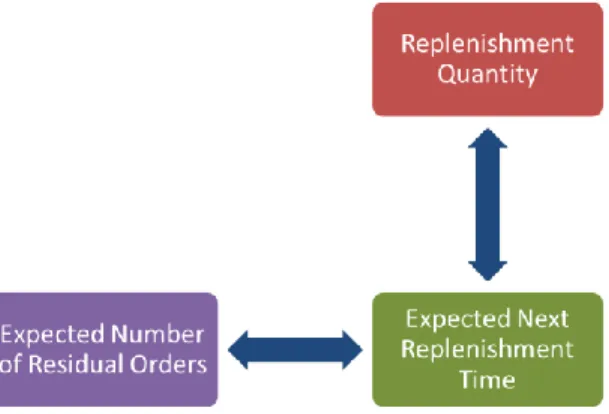
We know that our selection of replenishment quantity will affect the expected next replenishment time and expected number of residual orders. The relation is shown at Figure 3.1.

Figure 3.1 Relation between replenishment quantity decision and its effects.

Every replenishment order affects the remaining replenishments, hence to find replenishment quantity for only one interval needs to solve the consecutive problems as well. Hence decision to replenishment quantity needs the residual time into consideration. As we see every decision to replenishment quantity needs solving the subproblem between and .

Note that the replenishment quantity belongs to a large set and the expected next replenishment time is continuous, hence we can find and set the expected number of residual orders to find others.

(39)

29

Note that subproblem between and is a smaller version of the original problem, where we are deciding demand at time 0, when the time horizon is between and .

Solving this subproblem optimally has same complexity to solve the real problem. Therefore, we simplified the subproblems as follows: If we assume that the demand during residual time is deterministic and equal to demand rate , we can

solve the subproblem. Hence for an arbitrary time interval , the demand is known and fixed to ∫ . We know that the deterministic subproblem (DS) can be solved optimally if the total number of remaining replenishment is fixed. Therefore, starting from to a sufficiently large number , we can calculate the total cost for deterministic subproblem and then select the one which gives minimum total cost. This approach is suggested by Johnson and Montgomery [18] to solve Continuous Review Lot Size Problem. Trying various values is also suggested in their study. Note that, we are looking for the best selection of “expected number of residual orders” and then finding the expected time of next replenishment and finally the replenishment quantity. Deterministic Subproblem

Assume that total number of remaining orders is .

In this step, we will find the optimal solution to the deterministic subproblem (DS) between to with deterministic demand rate. Define represents time.

We denote is the total cost of optimal selection of replenishment times for deterministic subproblem, starting from . For any selection of replenishment times { } the total cost is denoted as where superscript

D represents deterministic problem. By using expectation on demand rate, expected total cost between and becomes;

(40)

30 ∑ ( ( ) ( )) ( ) ∑ ( ) ( ) ∫ ∫ (11)

Taking partial derivatives of this term with respect to ’s where { } gives optimality conditions. In optimal solution of ordering times the resulting terms must be equal to zero. This gives nonlinear conditions.

For

( ) ( ) ( ) ( ) (12)

For

( ) ( ) ( ) (13)

There are unknowns with equality conditions since we set for

(41)

31

found by using mathematical software. Johnson and Montgomery suggest setting a value for and then solving all remaining variables. If last condition does not satisfy equality another value of should be selected [18]. These conditions can be solved by

using mathematical software.

Since we know the optimal solution for the deterministic subproblem with orders, we can simplify the total cost term. Now, best total cost for deterministic subproblem with n orders can be defined as;

{

} ₍₁₄₎

Determining Replenishment Quantity based on DS Solutions

As discussed before, we can solve DS optimally for any given . Iterating from to a sufficiently large upper bound N gives the optimal number of orders, which is denoted by . A lousy selection of N can be calculated as follows:

( ) (15)

where we compare total setup cost with the total backordering cost of extreme solution where all residual orders are backordered.

We can write;

(42)

32

After selecting best solution to expected number of residual orders, one can calculate the ordering quantity. For optimal , we have . Then replenishment quantity for order is;

(17)

which corresponds to expected demand until expected next immediate replenishment time.

3.2.2.2. Myopic Order-up-to Level Decision

As discussed before, we can select the review period length among a set of finite candidates. This alternative may represent real-life conditions better since most of business applies periodic replenishments.

For each period length in the candidate set, we will define and solve a subproblem. Since these subproblems are considerably smaller than the subproblems we solved before, we don’t need to assume deterministic demand for these problems. We denote for the candidate set. For each candidate , define the subproblem between . Order-up-to level for any will be the smallest integer, which satisfies

the service level derived by holding and backordering cost parameters. Denote

∫

as the expected demand during review period. We will assume that the inventory position at the beginning of the period is equivalent to smallest integer, that satisfies service level derived by holding and backorder cost parameters. Let is the jth

(43)

33

candidate in the set . Let, is the replenishment quantity for candidate at time . Then,

{ ∑

} (18)

which is the same solution to newsvendor problem assuming demand follows Poisson distribution with rate . After solving all subproblems we will select the one give the minimum cost per unit time. Then, for we can find expected total cost by using following equation.

( ) ∑ ( ( ) ) ( )

(19)

where is the expected holding and backordering cost between and where starting inventory level is . This cost can be calculated by using order statistics of the Non-homogeneous Poisson Process.

Then total cost per unit time is simply

( ) ( ) (20)

For each element in the candidate set , we get . Here, we will select the best as which satisfies

(44)

34

{ ( ) } (21)

Now, we have the best solution for the myopic subproblem. Let is the index of selected period length. Then the order-up-to level is,

₍₂₂₎

After finding our order-up-to level, now we can define the real replenishment quantity, such as:

(23)

3.2.3. Last Order Problem

In section 3.2.2.1, we see how replenishment quantity can be chosen by solving deterministic subproblem for the residual time horizon. Remember that, we were solving deterministic subproblems for fixed number of residual orders. When we are sufficiently close to end-of-horizon , we can solve the stochastic subproblem without simplifying the stochasticity. We will call this problem as “Last Order Problem” (LOP).

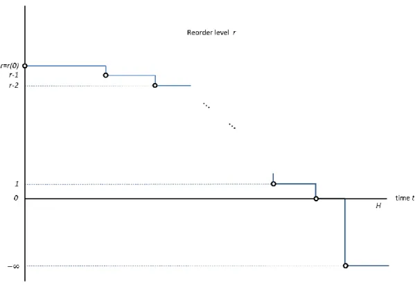
As we prove in section 3.2.1.3, reorder levels are non-increasing function of time. On top of that, if we assume that demand rate is a continuous, non-increasing function of time, then these reorder levels are step functions with certain break points.

(45)

35

Figure 3.2 Behavior of Reorder Level during Final Phase when Demand Rate is Non-Increasing Function of Time

At time , the order up to level will become minus infinity with optimal number of estimated replenishments for sure. Therefore, instead of issuing an order, retailer may want to wait until the end of horizon and simply meet the all backordered demands with a single replenishment. Note that, the start of the last phase where may become earlier than H-L.

In their study, Teunter and Haneveld show a similar effect while describing the optimal policy [32]. He shows that optimal order-up-to level function will reach zero, and eventually become minus infinity, where not placing any order is the best option.

The reason for order up to level function takes minus infinity value can be reviewed as follows; assume that an arbitrary demand occurred in , which is smaller than .

(46)

36

Assume our inventory position drops to -1. Retailer has two alternatives. First one is not giving any order at time and pays the backordering cost until end of horizon, which corresponds;

(24)

The second option is giving an order at and meets the item at . Then, the cost becomes;

(25)

If then the best policy is not giving any replenishment order. Therefore, it is obvious that the optimal order up to level for is strictly below zero. In order to find optimal reorder level, let there is another demand arrives where inventory position drops to -2 at time . Since and , we get . Therefore best policy for this singular order is same as previous: do not issue a replenishment order. Clearly, it is same for all demand after here and it is easy to see that, procedure can continue until minus infinity. Therefore optimal reorder level is minus infinity. When the retailer approaches near to end of the planning horizon, best estimation for remaining orders will get closer to zero.

Based on this observation, when optimal number of estimated replenishment is less than 2, time until is sufficiently close for considering not giving any order until end of final phase. Moreover the residual stochastic subproblem can be solved.

(47)

37

In this step we will compare expected total cost of two alternatives. First one is placing any order at time . Without loss of generality, assume that we will place an order with size of . Then, expected total cost between and will be;

(26)

Denote the demand between and is

( ∫

)

Then we can expand total cost formulation as;

(( ) ) ( [( ) ])

( )

(27)

where represent between and with an inventory position at . We can expand as;

( )

∑

(48)

38

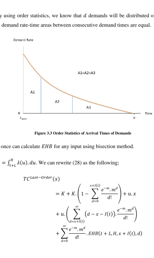
and by using order statistics, we know that demands will be distributed over horizon where demand rate-time areas between consecutive demand times are equal.

Figure 3.3 Order Statistics of Arrival Times of Demands

Then, once can calculate for any input using bisection method. Let ∫ . We can rewrite (28) as the following;

( ∑ ) ( ∑ ( ) ) ∑ (29)

(49)

39

As discussed above, our second alternative is not placing any order until . Modifying (30) we can write; _(∑ ) ∑ (30)

Note that, first term in the cost expression (31) represents the setup cost at the end of the horizon which is dependent to demand between and which follows Poisson Process with rate .

3.3. Heuristics

3.3.1. First Heuristic; Based on the Expected Number of Residual Orders

Since we are dealing with a finite horizon problem, replenishment times and quantities affect the remaining orders. In finite horizon inventory problems, generally, replenishments are correlated with each other. Logic behind this policy is based on this observation. In order to shape our policy, we are solving a deterministic subproblem for the remaining time horizon.

We know that deterministic demand variation of the problem can be solved optimally for fixed number of residual orders as discussed in section 3.2.2.1. If it is known that there will be ordering points, then it leads optimality conditions using first derivatives. These conditions have a unique solution. This observation constitutes a basis

(50)

40

for determining the replenishment quantity in our heuristic. Shortly, in our first heuristic, a deterministic subproblem at each ordering time is solved by using optimality conditions, and results of the problem used for determining ordering quantity.

We assume that, retailer start the final phase with sufficient (optimal) inventory level. In other words, assume the inventory is ordered at time ‘– ’.

As stated before, this heuristic is a continuous review policy, which is a variant of classical reorder level, order up to level inventory policy.

(51)

41