Sectoral informality in Turkey

(1)

SECTORAL INFORMALITY IN TURKEY

A Master’s Thesis by YASİN DALGIÇ Department of Economics Bilkent University Ankara February 2010

(2)

(3)

(4)

SECTORAL INFORMALITY IN TURKEY

The Institute of Economics and Social Sciences of

Bilkent University

by

YASİN DALGIÇ

In Partial Fulfillment of the Requirements for the Degree of MASTER OF ARTS in THE DEPARTMENT OF ECONOMICS BİLKENT UNIVERSITY ANKARA February 2010

(5)

I certify that I have read this thesis and have found that it is fully adequate, in scope and in quality, as a thesis for the degree of Master of Arts in Economics.

--- Asst. Prof. Selin Sayek Böke Supervisor

--- Asst. Prof. Ümit Özlale

Examining Committee Member

---

Asst. Prof. D. Şirin Saraçoğlu Examining Committee Member

Approval of the Institute of Economics and Social Sciences

--- Prof. Erdal Erel Director

(6)

ABSTRACT

SECTORAL INFORMALITY IN TURKEY

DALGIÇ, Yasin

M.A., Department of Economics

Supervisor: Asst. Prof. Selin SAYEK BÖKE

February 2010

This thesis evaluates the sectoral based probability of informal employment and its possible determinants. By decomposing the effects of workers’ characteristics and sectoral features on probability of informal employment, new measures of informality degrees of sectors are calculated. These new informality measures provide an easy and understandable interpretation and comparison across sectors. These new measures suggest that people who work in agriculture (includes agriculture, forestry and fishing) and construction sectors are more likely to be employed informally, while financial (financial intermediation, real estate, renting and business activities) and mining (mining and quarrying) sectors are relatively more formal in terms of employment. Additionally, among the determinants of differences in the probability of informal employment, the share of male workers and the amount of sectoral credits over GDP are found to be significant.

Keywords: Informality, Social Security, Informality Differentials, Linear Probability Model, Feasible Generalized Least Square Method.

(7)

ÖZET

TÜRKİYE’DE SEKTÖREL KAYITDIŞILIK

DALGIÇ, Yasin

Yüksek Lisans, İktisat Bölümü

Tez Yöneticisi: Yrd. Doç. Dr. Selin Sayek Böke

Şubat 2010

Bu tez, Türkiye’deki sektörel bazda kayıtdışı istihdam olasılığını ve bunun olası nedenlerini incelemektedir. İşçi karakteristiklerinin ve sektörel özelliklerin ayrıştırılmasından sonra sektörlerin yeni kayıtdışılık düzeyleri hesaplanmıştır. Bu yeni kayıtdışılık ölçüleri, sektörler arasında kolay ve anlaşılabilir yorumlar yapılmasına imkân vermektedir. Bu yeni ölçülere bakıldığında, tarım (tarım, ormancılık ve balıkçılık) ve inşaat sektörlerinde çalışan insanların kayıtdışı çalıştırılmaya daha yatkın oldukları bulunmuştur. Ayrıca, finansal (finansal aracılık, ev sahipliği, kiralama ve ticari faaliyetler) sektör ve madenciliğin (madencilik ve taşocakçılığı) kayıtdışı istihdam açısından göreceli olarak daha formal olduğu göze çarpmaktadır. Ek olarak, sektörlerde kayıtdışı istihdam olasılığı farklılıklarının nedenleri arasında sektörel banka kredilerinin Gayri Safi Milli Hâsıla’ya oranının ve sektörlerde çalışan erkek işçi oranının önemli olduğu bulunmuştur.

Anahtar Kelimeler: Kayıtdışılık, Sosyal Güvenlik, Kayıtdışılık Farklılıkları, Lineer Olasılık Modeli, Uygulanabilir Genelleştirilmiş En Küçük Kareler Metodu.

(8)

ACKNOWLEDGEMENTS

I would like to express my deepest thankfulness to Asst. Prof. Selin Sayek Böke not only for her supervision and guidance through the development of this thesis but also for unique helpfulness in times of need. I also would like to thank to Asst. Prof. Ümit Özlale and Asst. Prof. D. Şirin Saraçoğlu for their valuable comments on my thesis.

My thanks should also go for Assoc. Prof. Fatma Taşkın, Asst. Prof. Tarık Kara, Asst. Prof. Esra Durceylan-Kaygusuz and our secretary H. Meltem Sağtürk for their continuous support, encouragement and motivation during my Master’s degree.

I am especially grateful to all of my friends for their close friendship in the really hard times I lived through.

Finally, and most importantly, I would like to thank to my family for their endless love and support.

(9)

LIST OF TABLES

1. Table 4.1.1: Informal Employment Share of the Variables (%)……..……22 2. Table 4.2.1.1: Effects of Worker’s Characteristics and Working Sector on Probability of Being Informal……….26 3. Table 4.2.2.1: Marginal Probabilities…...………...33 4. Table 4.3.1: Normalized Informality Differentials for LPM and

Probit……….39 5. Table 4.3.2: Percentage Change in the Informality Differentials by Sector (2000 to 2008)………...……...42 6. Table 4.4.1.2: Regression Results with Feasible Generalized Least Square (FGLS)………...49 7. Table 4.4.1.3: Feasible Generalized Least Square Regressions with

additional variables of Real GDP Growth and Real Effective Exchange Rate ………51

(12)

LIST OF FIGURES

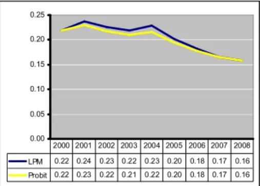
1. Figure 4.3.1: Employment Weighted Average Informality Differentials for LPM and Probit Regressions………..………38 2. Figure 4.3.2: Normalized Informality Differentials with LPM………40 3. Figure 4.3.3: Normalized Informality Differentials with LPM………40

(13)

CHAPTER I

INTRODUCTION

The term informality means different things to different people, but almost always with negative connotations: unprotected workers, excessive regulation, low efficiency and unfair competition, evasion of rule of law, underpayment or nonpayment of taxes and work underground or in the shadows1. Having no common description has given rise to usage of many terms in informality definition by scholars.

Feige (1990) defines informality as follows: “…when economic agent’s actions fail to adhere to the established rules or are denied their protection, the agent is regarded as a member of the informal sector of the economy”. Assaad (1987) and Portes (1994) state that the important characteristic of informality is the noncompliance with legal and administrative regulations rather than the social regulations. Maloney (2004) characterizes the informal sector as consisting of “small-scale, semi-legal, often low-productivity, and frequently family-based, perhaps pre-capitalistic enterprises”.

Schneider and Enste (2000) use the term “shadow economy” instead of informality and they broaden the definition as all market based legal production of

1

See the report Informality, Exit and Exclusion by Perry et al. (2007) which was published by the World Bank. The report concentrates on the countries in Latin America and Caribbean.

(14)

goods and services that are deliberately concealed from public authorities to avoid payment of income or value added taxes, to avoid payment of social security contributions, to avoid having to meet certain legal market standards, such as minimum wages, maximum working hours, safety standards, etc. and to avoid complying with certain administrative procedures such as completing statistical questionnaires or other administrative forms.

The International Labor Organization (1993) describes the informal sector consisting of economic units “with low level of organization with little or no division of labor and capital as factors of production on a small scale and mostly based on personal and social relations rather than contractual arrangements”2. In our study we will focus on the “noncompliance with the legal and administrative regulations” view of informality and use social security non-registration of workers as a measure which complies with the definitions that Asaad (1997) and Portes (1994) use.

Since informal activities are seen as a drag on productivity and growth of the economy and may lead to erosion of the functioning and the legitimacy of market and equity enhancing institutions, evaluation and measurement is important for policy implications and in turn for the well-being of the economy. Moreover, the social part of the incidence is also a central issue since jobs in the informal sector lack a sheltering mechanism to families from adverse shocks, loss of jobs, illness or calamity3.

2_{This definition belongs to the International Labor Organization (ILO) Resolutions Concerning} Statistics of Employment in the Informal Sector Adopted by the 15th International Conference of Labor Statisticians in January 1993.

3

(15)

This thesis is organized as follows: Chapter 2 provides information about methods for estimating informality. In Chapter 3, the thesis will present the literature review about informality. Chapter 4 gives explanation about the data with some preliminary evidence about informality in Turkey. Moreover, I will also present the regression results related with workers’ characteristics and sector of employment in the probability of informal employment, and the methodology which is used for creating a new comparable measure related with the probability of sectors to employ people informally and compare the sectors using this new measure of informality. Additionally, Chapter 4 presents the possible explanations of the differences of sectors in terms of informal employment applying regression analysis using the new measures of informality of the sectors. Finally, in Chapter 5, I will present concluding remarks.

(16)

CHAPTER II

METHODS FOR ESTIMATING INFORMALITY

Despite the fact that measurement of the extent of informality is a very crucial indicator for the well being of the economy, due to heterogeneity in terms of its definition and lack of data, there is no certain answer on how to do so. Moreover, since most economic activities that are classified as informal are not captured by national accounts and official statistics, the disputes on exact measurements of informality are likely to persist in the literature in the near future.

Although the difficulty of measurement is obvious, there are several methods that have been enhanced in order to gauge the size of the informal economy. Garcia-Verdu (2007) classifies these methods into three: direct methods, indirect methods (indicator approaches) and the model approach4:

Direct approaches to measure informality use voluntary surveys or data from tax audits to construct estimates of total economic activity and its measured and unmeasured components.

4

This categorization and explanation of the methods are heavily based on the report of Informality, Exit and Exclusion by Perry et al. (2007).

(17)

These surveys usually ask respondents to pronounce their labor status, social security conditions or the degree of tax compliance in their industry. On the other hand, tax audit based approaches calculates the size of the informal economy using the difference between the income-stated tax returns and the exact level of income, which is usually found after an audit. The major problem with voluntary surveys is the degree of credibility of the answers. Furthermore, tax-audit-based methods are applicable only to a few countries due to lack of data5.

Indirect methods, which are based on macroeconomic indicators, are associated with the difference between the actual value of the macroeconomic variable and its account value. For example, one of these methods measures the difference between the GDP through income and expenditure sides, where the discrepancy is attributed to the informal economy. The main problem with the GDP method is that it may not give precise results in the economies with high saving rates and transfer payments to abroad. Another method in indirect measurement of informality is the electricity consumption approach. Kauffman and Kaliberda (1996) propose that the difference between the growth rates of GDP and electricity consumption can be attributed to the growth of the informal economy. Although this approach has been used by many authors6, it has some shortcomings. For example, it does not account for the technological improvement in machinery and in order to compute the difference one needs to have a base year where informal economy is insignificant. The third method is the currency demand approach where the main purpose is to detect the discrepancy between the estimated values of the specified money demand equation and the observed values

5

Schnedier (2005) uses tax audit based approach for US and Sweden. 6

(18)

from actual data7. But this method has also been criticized due to assumptions such as a common velocity of money circulation between official and unofficial economies, only cash transactions in the unofficial part of the economy or a base year where the extent of the unofficial economy is zero8.

The third and last group includes the Multiple Indicator - Multiple Cause (MIMIC)9 models. In MIMIC models the main idea is that there is a system of equations where one group of equations includes the effects (or indicators) as a function of the latent variable (informal economy in our case) and the other group models the informal economy as a function of the causal variables. Applying maximum likelihood estimation to the reduced form of the system of equations which are constructed from the indicator variables and causal variables, the size of the informal economy is estimated. The model is a popular one among the others since it enables one to incorporate several different causal factors that influence underground activity and to determine their relative significance. Moreover, it allows one to take into account several different “signals” of underground economic activity simultaneously10. However, this approach is also subject to many criticisms; for example Smith (2002) and Hill (2002) state that the model should have relevant causal and indicator variables but there are no common economic theories to classify them. Moreover, Breusch (2005) shows that time path estimation of the informal economy for Canada during the period 1976-1994 using this method leads to wrong results; the results mostly reflects price inflation and real growth rate of the related country rather than the size of the informal economy.

7_{See Schneider (1986).}

8

See Thomas (1999) and Schneider (1986) for criticisms of the method. 9

A simple explanation of the theoretical model is available at Breush (2005) and Macias (2008). 10

(19)

In this study, we will use the direct approach method by utilizing the social security registration information of the respondents in the Labor Force Household Survey Yearly Dataset for the period 2000-2008 for Turkey. The information regarding the social security registration status of the individuals provides us accurate information as a measure of informality which makes our measurement relatively straightforward and more precise compared to the indirect methods and MIMIC model. We have the advantage of the truthfulness of the respondents; since the survey has a legal side and people might be subject to sanctions in case of false information. Besides, workers do not have obvious incentives to report that they are formal when they are informal as opposed to firms’ incentives to answer similar questions (since hefty penalties can be imposed on firms)11. So, this analysis overcomes the criticisms regarding surveys in general, where the respondents might not reveal the truth in their responses. As the survey is carried out by the legal authorities and there is a punishment for false information, these concerns are much less regarding this specific survey. Moreover, we have weights of the individuals for each year to have projections of the population which allows us to make more reliable inferences related with the whole population, not only for the sample size.

11

See Catao, Pages and Rosales (2009). They also state that using social security registration data for the measure of informality is highly correlated with other economy-wide the measures of informality.

(20)

CHAPTER III

LITERATURE REVIEW

Besides the measurement attempt, there is also a very large literature concentrating on the determinants of the informal economy. Below I will provide an overview of the literature, with a focus on the studies on informality in Turkey.

3.1. Determinants of Informality

3.1.1. Explicit and Implicit Taxes

While demand for greater flexibility, autonomy and entrepreneurship motives, risk taking, family tradition and mobility opportunities can be counted as voluntarily decisions for choosing informal sector, Blau (1987) and Maloney (1999) state that being short of human capital particular to a work or a firm may force people to prefer informal works. Loayza (1997), Azuma and Grossman (2002) and Dabla Norris et al. (2008) suggest that since formality imposes fiscal burdens on a firm such as taxes or costs of complying with regulatory requirements (for example social security contributions), firms try to operate informally by taking the risk of penalties.

(21)

In their empirical work, Friedman et al. (2000) evaluate 69 countries12 from very different regions and find that higher tax rates are associated with less informal activity as a percent of GDP13. They also evaluate corruption and they find that it is associated with more informal activity in view of the fact that entrepreneurs try to avoid formal work to reduce the cost of official procedure. On the other hand, Schneider and Enste (2000) estimate the size of the shadow economy for 76 developing, transition and OECD countries and find that informal activity is strongly related to increasing burdens of taxation, social security contributions and the corruption level in the economy.

Ihrig and Moe (2000) also investigate how tax policy affects the size of informal sector and tries to quantify the cost of it using a dynamic model. Sarte (2001) analyzes the link between the rent-seeking bureaucracies and the size of the informal economy in a theoretical perspective and concludes that because of the rent seeking bureaucrats, firms try to go informal. In their 75 country cross country panel data regression analysis, Loayza etal. (2005) finds that a heavier regulatory burden, particularly in product and labor markets induces informality.

3.1.2. Financial Development

Dabla-Norris et al. (2008) investigates the effect of financial market development and the quality of regulatory burden on informality as well for more than 4000 firms in 41 countries and discover that both of these aspects also do play a role in driving informality. Straub (2005) evaluates the credit market channel of the informal economy in a theoretical manner. Building a model of

12_{See related paper for the list of countries.} 13

This result can be contradictory to what one expects but the authors express that the main reason can be that at least for this set of countries, higher tax rates may generate revenue that provides productivity enhancing public goods and a strong legal environment.

(22)

firms’ choice between formality and informality, he finds that complying with costly registration procedures allows the firms to benefit from key public goods, enforcement of property rights and contracts that finally result in the participation in the formal credit market. Moreover, Koeda and Dabla-Norris (2008) affirm this fact and find evidence that informality is robustly and significantly associated with lower access to and use of bank credit for firms in 26 transition countries in Eastern Europe and Central Asia.

In a recent work, using the National Household Survey Data for the period 2002-2007 and social registration condition of workers and formal employment contracts data of workers as measures of informality, Catao, Pages and Rosales (2009) also find that financial deepening increases the formalization rate in Brazil. They suggest that since formal credit saves on higher costs and legal insecurity of informal credit markets, firms’ incentives to become formal to get cheaper credit from banks increases.

3.1.3. Trade liberalization

The trade aspect of informality is also investigated by many researchers. Among them, Currie and Harrison (1997), where they used micro-level data on individual enterprises, examine the trade reform in Morocco during the 1980s and find that comprehensive trade liberalization led to a rise in firms’ hiring of more temporary workers (who are mostly informal). Additionally Pavcnik and Goldberg (2003) study the relationship between trade reforms in Brazil and Colombia and the size of the informal sector. They test the hypothesis that increased foreign competition in developing countries leads to an expansion of the informal sector. They find that there is weak evidence, only for Colombia, and for the period

(23)

preceding a major labor market reform that increased the flexibility of the Colombian labor market. Another study by Aleman-Castilla (2006) evaluates the relationship between import tariff reduction under NAFTA and informality for the period 1988-2002 for Mexico. Using social security coverage data as an indicator of informality, they find that by inducing the most productive formal firms to engage in trade, trade liberalization could reduce the incidence of informality through the increase for the labor demand from the less efficient informal firms to more efficient formal ones, increasing the employment share of the formal sector14.

3.2. Informality in Turkey

Studies on informality in Turkey have increased since the early 1990s. Many of these studies have focused on estimating its size. Among those, Yılmaz and Öğünç (2000), Çetintaş and Vergil (2003), Yurdakul (2006) and Akalın and Kesikoğlu (2007) use monetary approaches to estimate the informal economy in Turkey. Temel et al. (1994) estimate the size using the indirect methods while Savaşan (2003) and Schneider and Savaşan (2007) use Multiple Indicator - Multiple Cause (MIMIC) model. Us (2005) evaluates informality in Turkey by using the Tax Auditing Approach (Direct Method), the Employment Approach, the GNP Approach and the Monetarist Approach (Indirect Methods) and compare the results; concluding that it is very difficult to focus on only one method since calculated sizes differ across methods of measurement.

14

This is a contradictory result compared to study of Pavcnik and Goldberg (2003), and author ties to the fact that liberalization of trade in Brazil and Colombia has been rather different from the 1990s Mexican experience (See the related paper).

(24)

Tansel (1999) evaluates the choice of informality among the wage earners in terms of being covered by a social security program or not and expresses that both for men and women, people with more education are more likely to have social security coverage. Additionally, she also states that people who live in urban areas are more likely to have social security coverage compared to people in

rural areas. Bulutay and Taştı (2004) analyze the informality trend in Turkey with

respect to different definitions15 using two different datasets; Household Labor Force Surveys (1990-1999) and Urban Areas Small and Unincorporated Enterprise Survey for the year 2000 and they find that younger people and less educated individuals work tend to more informally16.

Saraçoglu (2008) studies informal sector in a dynamic model and finds that informality can successfully be reduced by reducing taxes on employment in the formal sector. Another study by Schneider and Savaşan (2006) address the sectoral and micro aspects of informality using data from the textile sector in Turkey. Using a questionnaire related with the informal hiring in the textile sector in 2005, they find that high competition, the skill structure of the employees and the size of the firms are important factors of the textile firms hiring informally.

The main findings of the studies for other countries and Turkey generally comply with each other. For example, Pavcnik and Goldberg (2003) also confirms Bulutay and Taştı (2004) by finding that more educated people and elder individuals tend to work more formally compared to less educated people and single individuals for Brazil. In fact this is not a very surprising result since one can expect that education and skill provides more work opportunities to people

15

See the related paper for various definitions.

16_{In their study, Bulutay and Taştı (2004) also analyze the sectoral composition (industry, trade} and service) of formal and informal people. But this analysis is only based on the number, share and gender of the formal and informal workers and remains very descriptive and limited to three very broad sector classifications.

(25)

compared to less educated or less skilled people. Moreover, one can also expect that younger people also tend to work more informally since the elder people consider health care opportunities for their family members compared to younger people.

The positive effect of reducing the tax on employment for the formal employment tend to be a general pronouncement for the studies Loayza (1997), Azuma and Grossman (2002) and Dabla Norris et al. (2008) and Schneider and Enste (2002) with Saraçoğlu (2008) which makes us to consider heavy tax burden as a general problem for the firms, which forces them to operate informally.

There are also several administrative reports regarding informality in Turkey. For example, The 8th Five Year Development Plan has a special report providing comprehensive information about the causes, consequences, methods for determining its size, including many of its perspectives like national income, employment, tax and illegal activities17.

In another report, Özlale (2008) presents valuable information about the size, institutional and macroeconomic determinants of informality and sector-based opinions of firms regarding informality. He emphasizes that there is an increasing trend in informality in the crisis years (1994 and 2001); and the weak regulations in tax policies, the cost of employing and social security contributions of the formal workers seem to be the primary problems for the firms and construct basis of informality in Turkey.

In this thesis, we will analyze informality not only at the national level but also at the sectoral level and examine its determinants by following the

17

(26)

methodology of Pavcnik and Goldberg (2003)18. In doing so, we will also be able to discuss the personal characteristics that lead to informal employment of an individual. While there are ample studies on informality in Turkey, there is no study that looks into informality at the sector level for a wide range of sector definitions (Bulutay et al. (2004) study only 3 sectors and Schneider and Savaşan (2006) only look into the textile sector). It is of interest to further understand the dynamics and determinants of informality in Turkey, across sectors and across time (2000-2008).

Using the Household Labor Force Survey Data for the years 2000-2008, we will provide current dynamics of informality in Turkey, both at the individual and sectoral level. This is the first study that combines these two aspects for Turkey and allows a synchronous discussion of the factors that play a role in an individual’s informal employment and those that influence the extent of informality at the sectoral level. From the individual worker’s point of view, I will investigate the role of worker’s characteristics like age, age-squared, sex, marital status, education level and living in urban and rural areas on an individual’s working informally. Upon decomposing worker’s characteristics and sectoral informality, we will create a new measure of relative informality levels of each sector and a hypothetical sector that represents “the average of all sectors” which is the main aim of this thesis. This will allow identification of whether there are sectors which are ridden by “chronic informality”19. Then using these sectoral informality measures, I will also try to determine the underlying reasons of the high levels of informality in these sectors using several variables that have

18

This methodology allows us to decompose personal and sectoral characteristics of informality. Moreover, we will also be able to evaluate the determinants of the sectoral informality levels. 19

This definition belongs to the author. By “chronic informality” author means the sectors that have persistent high levels (above the “average”) of informality levels for a long period (nine years in our data set) stemming from the reasons apart from workers’ characteristics.

(27)

possible explanations in the differences probability of informal employment across sectors. Evaluating all these may guide implementation of effective policies on a sectoral basis to policymakers.

(28)

CHAPTER IV

DATA AND METHODOLOGY

In this study, the Turkish Household Labor Force Survey (HLFS) annual data will be used20. It covers the period 2000-2008 and it is a cross sectional data21. The survey is prepared on a monthly basis and the results are published every month. But when the data set is prepared for a specific month, for instance February, three monthly data sets are combined (January and March are also added) by taking the weights of each month into consideration. The survey is prepared as follows: surveyors go to the same families four times in eighteen months. For example, a family, which is visited on January 2000 for the first time, will be visited after three months (in April). The third visit will be after nine months (in January 2001) and the fourth visit will be in (April 2001). If the visit on January is the second visit to that family, then the third visit will follow after nine months. This means, the same people are counted twice in the same year’s data set. Since we do not have the data of each individual specifically, we use data

20_{Quarterly data is not publicly available.} 21

Although the data sets for 2000-2003 and 2004-2008 are different in number of questions and their categories, observations and regions, I standardize the categories of the variables that are used in the regressions. Moreover, the data set we use is weighted by taking base year as 2000.

(29)

set as cross-section on yearly basis (same people are counted as if they are different)22.

The surveyors ask a set of questions to all members of the families regarding their socioeconomic characteristics. The surveys contain useful information about a person’s age, marital status, gender, level of education, employment activities, whether he/she has a social security registration, his/her sector of employment and several other variables.

This study does not take people into account who are under the age of 15 due to the labor force definition of the Turkish Statistical Institute (TURKSTAT). Our informality measure is based on the question of “Are you registered in Social Security?”23. People who are registered are denoted as 0, and those who are not are denoted as 1. We will regress this informality measure on socioeconomic factors like gender, level of education, age, marital status and dummy variables capturing seven main sectors we have in the data set24 using the linear probability model (LPM), linear probability model with weighted least squares and the Probit model, respectively. Upon obtaining the coefficients of the regressors, we will apply a two stage restricted method which is presented by Haisken-DeNew and Schmidt (1994) and used by Pavcnik and Goldberg (2003) in order to find the main informality measure that we focus on.

The Linear Probability Model (LPM) method is used while regressing the probability of an individual being formally employed on personal characteristics

22

For more information about the LFHS, see report Labor Force, Employment and Unemployment Statistics available on http://www.tuik.gov.tr/IcerikGetir.do?istab_id=134.

23

The social security registration of the workers as a measure of informality is included in direct methods of calculating informality and also used by Pavcnik and Goldberg (2003), Attanasio et al. (2004), Aleman-Castilla (2006) and Henley et al. (2009) in their studies.

24_{One category is dropped in order to prevent multicollinearity. In fact many sectors in the data set} are combined and this combination results in remaining nine sector categories. Among them, one category of combined sectors is dropped (electricity, gas and water supply) since in 2001; all people in this category are reported as working formally.

(30)

and sectoral dummies as in the work of Pavcnik and Goldberg (2003). I will also apply linear probability model with weighted least squares and probit regressions for robustness purposes due to several theoretical problems associated with the LPM (heteroskedasticity, and the fact that fitted, i.e. predicted probabilities may lie outside the range of 0 and 1).

We will define the regression model as follows:

P(informal)= y = Zδ + Xβ + ε (1)

In the model, the dependent variable is the probability of being formal (y=0) or informal (y=1) (i.e. having a social security registration or not). Z includes variables of personal characteristics and area of residence of the individual, where the variables are listed as follows:

Gender (male): This variable is assigned the value of 0 if the individual is

female, and 1 if male. Existing literature does not have a common ground related with the effect of this variable on probability of formal or informal employment. For instance, while Maloney (2004) states that women are over-represented in the informal labor markets of developing countries, Pavcnik and Goldberg (2003) and Aleman-Castilla (2006) argue that men are more likely to be employed informally in Colombia and Mexico.

Age (age_groups): We have 12 age categories in the data set. The first

category is eliminated since it includes individuals who are below the age of 15 and are out of the labor force according to the definition of TURKSTAT. The second category includes people who are between the ages of 15 and 19. The remaining categories are constructed with 4 year intervals as in the second category (for example the third category consists of individuals who are between the ages of 25 and 29 etc.). Only the last category includes a wider range; this

(31)

category includes all people who are 65 years old and above. The literature expresses that young people are generally employed informal25. Bulutay and Taştı (2004) confirm this for Turkey; they state that people in younger ages are more likely to be employed informally. However there are some works which express that the effect of age on the probability of informal employment is not very clear. For example, Maloney (2004) stresses that people in older ages may desire to be self employed after accumulating experience in formal works so that the effect of age on the probability of formal or informal employment can be difficult to evaluate.

age_groups2: This variable is calculated by taking the square of

age_groups variable in order to see the marginal effect of age increase, whether it has a decreasing or increasing contribution to the probability of working informally.

Level of education (educlev): In the data set, we have 7 categories of

education levels; illiterate, incomplete basic education, primary school, secondary and vocational education, general high school, vocational high school and tertiary education (faculty, university and masters/PhDs.). Individuals with no, or minimum education are mostly expected to be informal wage employees26. The works of Bulutay and Taştı (2004) and Pavcnik and Goldberg (2003) confirm this; the effect of education is found to be negative in informal employment in their studies.

Marital status (married): People who are married during the period of

the survey are assigned the value of 1 and other people are assigned the value of 0. The effect of marital status of workers on the probability of formal or informal

25

See Jütting et al. (2008) for more information related with the literature. 26

See report “Informal Employment Reloaded” byJütting et al. (2008) for more detailed literature survey about education available at www.oecd.org/dataoecd/4/7/39900874.pdf

(32)

employment is also uncertain in the literature. For example Pavcnik and Goldberg (2003) find that marriage is an important determinant of informal working and married people are more likely to be employed informally in Brazil and Colombia whereas Perotti and Puerta (2009) observe that married people are more likely to be employed formally in Bulgaria.

Region of residence (urban): This variable stands for the area of

residence of the individual. If the individual lives in a city, it is assigned the value 1 and 0 otherwise (if he or she lives in the rural area). Bulutay and Taştı (2004) states that in urban areas educated people are more likely to be employed formally compared to less educated people. By adding this variable into regressions, we will be able to evaluate the individual effect of living area in the probability of informal employment.

The X vector includes our eight sectors: agriculture, forestry, hunting and fishing (agr), mining and quarrying (min), manufacturing (manuf), construction (cons), wholesale and retail trade, repair of motor vehicles, motorcycles and personal and household goods, hotels and restaurants (whole), transportation, communication and storage (trans), financial intermediation, real estate, renting and business activities(fin) and other social, community and personal service activities; public administration and defense; compulsory social security, excluding armed forces; education; health and social work (social)27.

27

From now on, we will use names agriculture sector for “agriculture, forestry and fishing”, “wholesale sector” for “wholesale and retail trade, repair of motor vehicles, motorcycles and personal and household goods, hotels and restaurants”, “transportation” for “transportation, communication and storage”, “financial sector” for “financial intermediation, real estate, renting and business activities” and “social sector” for “other social, community and personal service activities; public administration and defense; compulsory social security, excluding armed forces; education; health and social work” instead of writing the whole group of sectors each time in order to save space.

(33)

4.1. Some Preliminary Evidence

The Table 4.1.1 presents the informal share of the workers for the related variables. We see that, in all years, informal share of working women in female employment is higher than the working men in male employment. Over the period, we also observe that the informality shares of both men and women decreases generally; but the increase in informal shares for both men and women in 2001 (crisis year) is remarkable. Single people also have higher shares of informal employment compared to married people. The people who work in urban areas tend to have higher shares of informal employment compare to rural areas.

The distinction among sectors in terms of informal employment shares is also noteworthy. For instance, the percentage of informally employed people in agriculture is higher than other sectors; approximately 90% of the people in this sector work informally. Construction sector also has high shares of informal employment; but not as much as agriculture does. The informal employment share in this sector tends to be stable; roughly 60% during the period. Wholesale and transportation sectors have relatively low shares of informal employment compared to agriculture and construction; but their level is higher than that in manufacturing, finance, social sector and mining. The informal employment shares of financial sector and social sector are similar to each other and follow similar patterns. Mining sector has the lowest share of informal employment share among all sectors, and this share does not exceed 16% over the whole period.

Informal employment share decreases as with more education. For example, the informal employment share of illiterate people is generally higher than 90% during the period and this share is below 10% for the people with

(34)

tertiary education. It means that while 9 of 10 illiterate people are employed informally, only 1 of 10 people with high education is employed informally.

The informal employment shares with respect to age groups are also essential to evaluate; since one cannot say that “as age increases, informal share of workers decreases or increases”. The table shows us that informal employment shares decrease as people get older but until up to the ages of 30-34; then it starts to increase. The lowest informal employment share belongs to people who are between 30 and 35. The people, who are between 15 and 19 and above 65, have similar levels of informal employment shares between 2000 and 2006.

Table 4.1.1. Informal employment share of the variables28 (%)

28

For example, in 2000 the value of the male variable is 45. This means that 45% of male workers are working informally.

Group Variable 2000 2001 2002 2003 2004 2005 2006 2007 2008 male 45 46 45 45 47 44 43 40 38 female 70 74 73 72 71 68 66 61 59 married 48 50 49 49 50 48 47 44 43 not married 61 63 63 61 62 58 55 49 45 urban 74 76 73 74 74 69 68 69 68 w o rk e r c h a ra c te ri s ti c s rural 29 32 34 33 36 36 35 34 31 agr 89 92 90 91 90 88 87 88 88 min 9 8 12 15 14 13 16 15 13 manuf 27 28 32 31 31 32 32 30 26 cons 66 62 62 64 66 64 62 60 56 whole 38 40 43 42 44 44 43 42 40 trans 31 33 34 34 39 39 40 38 36 fin 14 16 19 20 21 21 20 18 16 w o rk in g s e c to r social 11 12 14 14 17 18 18 18 17

(35)

Table 4.1.1. Informal employment share of the variables (%)(cont’d)

Source: LFHS

In the following section, we will be concentrating on workers’ characteristics and sector of employment in terms of probability of working formal or informal using LPM and Probit29 in order to see the individual effects of the related variables.

4.2. Effects of Worker’s Characteristics and Working Sectors on

Being Formal or Informal using LPM and Probit Regression

In this section we want to evaluate workers’ characteristics and the sector of employment on the probability of being informal. Using the LPM and Probit

29

I have also used LPM with Weighted Least Squares for robustness purposes. Results suggest that some of the values of coefficients in some years have opposite signs compare to LPM and probit (for example urban coefficient in 2000 and 2005 has a positive sign; meaning that people who live in urban areas are more likely to be employed informally, which is an unexpected result compare to LPM and Probit). This sharp distinction probably stems from the adjustments method (WLS) because adjustment method may result in some problems like substantial increases in the magnitude of most coefficients as well as increases the usual measure of R2_{(see Debertin,} Pagoulatos and Smith (1980) for more information). For this reason, I prefer to use the coefficients that are derived from LPM in the rest of thesis rather than LPM with WLS (Probit regression results are very similar to each other as in the study of Pavcnik and Goldberg (2003)).

illiterate 89 94 94 95 94 94 95 95 94 incomplete basic education 84 85 84 88 87 86 86 87 86 primary school 61 63 64 65 64 61 60 56 55 secondary and vocational education 40 42 45 47 50 51 50 49 48

general high school 25 27 28 29 32 31 32 30 28

voc. high school 22 24 24 25 27 27 25 24 22

e d u c a ti o n l e v e l tertiary education 5 7 8 8 9 10 9 10 9 15-19 79 84 86 86 86 84 82 79 76 20-24 57 62 62 60 63 57 54 48 44 25-29 43 46 45 43 45 41 40 34 31 30-34 40 40 40 40 43 39 37 33 31 35-39 40 41 40 41 42 40 38 35 34 40-44 38 39 39 40 43 41 40 36 35 45-49 46 48 48 49 49 48 47 47 45 50-54 56 62 61 60 61 60 61 60 60 55-59 66 68 71 74 71 72 73 74 73 60-64 70 77 77 83 80 80 81 84 84 a g e 65 and above 81 86 83 88 85 85 85 89 90

(36)

Regressions30, we get the summary statistics presented in the Table 4.2.1.1 below for the period 2000-2008. In the regressions, we use weight factors for population projections provided in the data set for every year which provides us more precise interpretations about the whole labor force in Turkey.

The results (with respect to LPM regressions) are as follows:

4.2.1. Worker’s Characteristics:

male: From regression results, we see that male workers are more likely to

work in the formal sector compared to female workers in all of the years. This can be attributed to the dominant role of men in the family for the responsibility of the household. That is, the male worker has to provide basic needs of all members of the family; he has to work, provide health care services etc. In this manner, one can expect that the male worker is likely to choose the job which provides social security registration among the alternatives. Moreover, the male worker can have more opportunities to choose among the alternatives compared to female worker, since some of the jobs are predominantly male oriented. For example, the male worker can work in mining or in construction sector, but the female worker is less likely to work in these kinds of jobs. Additionally, informal employment can be more preferable by women since they provide flexibility to be involved in family responsibilities. The regression results related to male variable are contradictory with the results of Pavcnik and Goldberg (2003) and Aleman-Castilla (2006), who find that men are more likely to be employed informally in Colombia and Mexico; but comply with the assessment of Maloney (2004).

30

Pavcnik and Goldberg (2003) use linear probability model in their regressions. Although they check their results with probit regressions, they continue to use linear probability model stating that the results are very similar to each other.

(37)

age_groups: Elder people tend to work formally more compared to younger

people and this feature is more apparent especially after 2005. This result supports the findings of Bulutay and Taştı (2004). Increase in age groups has a decreasing level of contribution to formal employment. The regression result related with age variable may be attributed to the fact that the first aim of people in younger ages is to find a job. But as they get older, they probably prefer to or look for the jobs that provide social security due to the concerns of family and retirement.

educlev: Education level of people also seems to be an important factor for

working formally. The regression results in the Table 4.2.1.1 shows us that higher educated people tend to work more formally in both regression models and for all years generally31. This result complies with the findings of Bulutay and Taştı (2004) for Turkey, Pavcnik and Goldberg (2003) for Brazil and Colombia and Aleman-Castilla (2006) for Mexico. It is highly possible that education provides more skills and more opportunities to people and they have more choices of jobs compared to people who are less educated. Moreover, one can also think that higher educated people have more qualifications compared to less educated and less skilled people so that employers may tend to provide formal jobs to those people in order to prevent their leave. For example, it is more likely that an engineer is employed formally compared to a manual worker if they both work in the construction sector.

31

(38)

Table 4.2.1.1. Effects of Worker’s Characteristics and Working Sector on Probability of Being Informal

Standard errors are in parenthesis.

*** indicates the explanatory variable is significant at 1% significance level. ** indicates the explanatory variable is significant at 5% significance level. R2

stands for the coefficient of determination of LPM and LPM with WLS. Pseudo-R2 stands for the coefficient of determination in probit regression. Dependent variable is “social security coverage”.

32

Since we have used population weights for the sample, number of observations for each year tends to become as in the parentheses.

LPM Probit Variable 2000 2001 2002 2000 2001 2002 constant 0.834*** (0.0006) 0.860*** (0.0007) 0.994*** (0.0007) 1.470*** (0.0025) 1.880*** (0.0030) 2.200*** (0.0029) male -0.086*** (0.0002) -0.083*** (0.0002) -0.101*** (0.0002) -0.425*** (0.0009) -0.504*** (0.0009) -0.537*** (0.0009) age_groups -0.087*** (0.0002) -0.099*** (0.0002) -0.118*** (0.0001) -0.324*** (0.0007) -0.429*** (0.0008) -0.476*** (0.0008) age_groups2 0.005*** (0.0000) 0.006*** (0.0000) 0.007*** (0.0000) 0.019*** (0.0001) 0.025*** (0.0001) 0.030*** (0.0001) educlev -0.068*** (0.0001) -0.068*** (0.0001) -0.073*** (0.0002) -0.286*** (0.0003) -0.303*** (0.0003) -0.299*** (0.0003) married -0.058*** (0.0002) -0.051*** (0.0002) -0.057*** (0.0002) -0.235*** (0.0010) -0.206*** (0.0011) -0.220*** (0.0010) urban -0.046*** (0.0002) -0.006*** (0.0002) -0.014*** (0.0002) -0.138*** (0.0009) -0.010*** (0.0009) -0.045*** (0.0009) agr 0.550*** (0.0003) 0.593*** (0.0003) 0.530*** (0.0003) 1.892*** (0.0014) 2.123*** (0.0014) 1.857*** (0.0014) min -0.056*** (0.0013) -0.058*** (0.0012) -0.040*** (0.0011) -0.147*** (0.0066) -0.259*** (0.0066) -0.106*** (0.0052) manuf 0.040*** (0.0003) 0.040*** (0.0003) 0.052*** (0.0003) 0.265*** (0.0013) 0.244*** (0.0013) 0.259*** (0.0012) cons 0.440*** (0.0004) 0.410*** (0.0004) 0.400*** (0.0004) 1.479*** (0.0016) 1.393*** (0.0017) 1.343*** (0.0017) whole 0.170*** (0.0003) 0.180*** (0.0003) 0.190*** (0.0003) 0.721*** (0.0013) 0.743*** (0.0013) 0.741*** (0.0012) trans 0.142*** (0.0004) 0.156*** (0.0004) 0.149*** (0.0004) 0.685*** (0.0017) 0.736*** (0.0017) 0.685*** (0.0017) fin 0.030*** (0.0005) 0.037*** (0.0005) 0.040*** (0.0005) 0.234*** (0.0023) 0.283*** (0.0022) 0.273*** (0.0021) Number of Observations32 84.038 (21.489.440) 85.318 (21.429.291) 85.078 (21.250.491) 84.038 (21.489.440) 85.318 (21.429.292) 85.078 (21.250.492) R2 and Pseudo-R2 0.450 0.477 0.435 0.385 0.426 0.386

(39)

Table 4.2.1.1. (cont’d)

Standard errors are in parenthesis.

*** indicates the explanatory variable is significant at 1% significance level. ** indicates the explanatory variable is significant at 5% significance level. R2 stands for the coefficient of determination in LPM. Pseudo-R2 stands for the coefficient of determination in probit regression. Dependent variable is “social security coverage”.

married: The probability that married people work informally is lower compared

to single people for all years. The reason for this fact can be that married people have more chance to search and choose formal jobs (especially if their husbands or wives are working). They may also prefer to search more among the jobs and work formally since the responsibilities of married people in their families are higher compared to single people. They have to provide social security not only

33

LPM Probit Variable 2003 2004 2005 2003 2004 2005 constant 0.991*** (0.0006) 1.000*** (0.0006) 1.369*** (0.0010) 2.296*** (0.0027) 2.178*** (0.0026) 3.421*** (0.0040) male -0.088*** (0.0002) -0.092*** (0.0002) -0.106*** (0.0002) -0.491*** (0.0009) -0.464*** (0.0009) -0.491*** (0.0008) age_groups -0.124*** (0.0001) -0.111*** (0.0002) -0.163*** (0.0002) -0.537*** (0.0008) -0.447*** (0.0008) -0.630*** (0.0010) age_groups2 0.008*** (0.0000) 0.007*** (0.0000) 0.008*** (0.0000) 0.036*** (0.0001) 0.029*** (0.0001) 0.034*** (0.0001) educlev -0.075*** (0.0001) -0.077*** (0.0001) -0.080*** (0.0001) -0.308*** (0.0003) -0.304*** (0.0003) -0.301*** (0.0002) married -0.060*** (0.0002) -0.070*** (0.0002) -0.069*** (0.0003) -0.225*** (0.0010) -0.265*** (0.0010) -0.246*** (0.0010) urban -0.008*** (0.0002) -0.012*** (0.0002) -0.011*** (0.0002) -0.030*** (0.0009) -0.041*** (0.0008) -0.034*** (0.0008) agr 0.545*** (0.0003) 0.510*** (0.0003) 0.469*** (0.0003) 1.912*** (0.0014) 1.736*** (0.0013) 1.580*** (0.0013) min -0.049*** (0.0013) -0.079*** (0.0012) -0.118*** (0.0012) -0.042*** (0.0058) -0.175*** (0.0051) -0.341*** (0.0049) manuf 0.044*** (0.0003) 0.023*** (0.0003) 0.017*** (0.0003) 0.242*** (0.0012) 0.139*** (0.0012) 0.138*** (0.0011) cons 0.410*** (0.0004) 0.393*** (0.0004) 0.365*** (0.0004) 1.371*** (0.0017) 1.257*** (0.0016) 1.180*** (0.0015) whole 0.181*** (0.0003) 0.178*** (0.0003) 0.158*** (0.0003) 0.718*** (0.0012) 0.653*** (0.0011) 0.593*** (0.0011) trans 0.145*** (0.0004) 0.157*** (0.0004) 0.151*** (0.0004) 0.672*** (0.0017) 0.638*** (0.0016) 0.615*** (0.0015) fin 0.055*** (0.0005) 0.032*** (0.0005) 0.025*** (0.0005) 0.361*** (0.0020) 0.227*** (0.0019) 0.206*** (0.0018) Number of Observations33 80.780 (21.047.648) 136.300 (21.707.579) 140.457 (21.966.068) 80.780 (21.047.649) 136.300 (21.707.579) 140.457 (21.966.068) R2 Pseudo-R2 0.445 0.410 0.378 0.397 0.360 0.329

(40)

for themselves but also for their spouses and for their children (if they have). This result complies with the findings of Aleman-Castilla (2006) for Mexico.

Table 4.2.1.1. (cont’d)

Standard errors are in parenthesis. *** indicates the explanatory variable is significant at 1% significance level. ** indicates the explanatory variable is significant at 5% significance level. R2

stands for the coefficient of determination of LPM. Pseudo-R2 stands for the coefficient of determination of probit regression. Dependent variable is “social security coverage”.

urban: The results of the regressions also suggest that people who live in

urban areas are more likely to have social security coverage compared to people who live in rural areas35. This can be related to the variety of work opportunities in the urban areas compared to rural areas, holding all other things constant.

34

35

LPM with WLS regression results show us that in 2001, 2005 and 2006, the coefficient of the urban dummy turns out to be positive, which is an unexpected result, as in the case of education level variable for 2000.

LPM Probit Variable 2006 2007 2008 2006 2007 2008 constant 1.132*** (0.0007) 1.150*** (0.0008) 1.100*** (0.0008) 2.447*** (0.0025) 2.565*** (0.0030) 2.486*** (0.0029) male -0.111*** (0.0002) -0.099*** (0.0002) -0.100*** (0.0002) -0.498*** (0.0008) -0.451*** (0.0008) -0.459*** (0.0008) age_groups -0.142*** (0.0001) -0.153*** (0.0002) -0.145*** (0.0002) -0.538*** (0.0007) -0.611*** (0.0008) -0.597*** (0.0008) age_groups2 0.010*** (0.0000) 0.011*** (0.0000) 0.011*** (0.0000) 0.038*** (0.0001) 0.047*** (0.0001) 0.047*** (0.0001) educlev -0.083*** (0.0001) -0.079*** (0.0001) -0.076*** (0.0001) -0.308*** (0.0002) -0.294*** (0.0002) -0.290*** (0.0002) married -0.057*** (0.0002) -0.045*** (0.0003) -0.037*** (0.0002) -0.203*** (0.0009) -0.158*** (0.0010) -0.137*** (0.0010) urban -0.019*** (0.0002) -0.032*** (0.0002) -0.038*** (0.0002) -0.063*** (0.0008) 0.109*** (0.0009) -0.132*** (0.0009) agr 0.435*** (0.0003) 0.422*** (0.0004) 0.425*** (0.0003) 1.468*** (0.0007) 1.430*** (0.0013) 1.420*** (0.0013) min -0.095*** (0.0011) -0.110*** (0.0011) -0.108*** (0.0012) -0.250*** (0.0046) -0.288*** (0.0046) -0.306*** (0.0050) manuf 0.012*** (0.0003) 0.001*** (0.0003) -0.017*** (0.0003) 0.124*** (0.0011) 0.095*** (0.0011) 0.026*** (0.0012) cons 0.333*** (0.0004) 0.320*** (0.0004) 0.287*** (0.0004) 1.080*** (0.0015) 1.034*** (0.0015) 0.947*** (0.0015) whole 0.144*** (0.0003) 0.136*** (0.0003) 0.130*** (0.0003) 0.548*** (0.0011) 0.526*** (0.0011) 0.508*** (0.0011) trans 0.156*** (0.0004) 0.137*** (0.0004) 0.126*** (0.0004) 0.622*** (0.0015) 0.563*** (0.0015) 0.531*** (0.0016) fin -0.002*** (0.0004) -0.0138*** (0.0004) -0.028*** (0.0004) 0.095*** (0.0017) 0.064*** (0.0017) -0.005** (0.0017) Number of Observations34 142.800 (22.236.997) 137.762 (20.639.881) 139.168 (21.102.287) 142.800 (22.236.998) 137.762 (20.639.881) 139.168 (21.102.287) R2 Pseudo-R2 0.368 0.364 0.392 0.320 0.323 0.330

(41)

Moreover, compositions of the working sectors may differ in urban and rural areas. For example, in rural areas numbers of farmyards are much higher than the urban areas so that it is more likely to have agriculture as the dominant sector compared to an urban area. Besides, one can also think that government controls and labor laws are more likely to be enforced by legal authorities in urban areas than rural areas which can increase the probability of formal employment in urban areas.

4.2.2. Sector of Employment:

Table 4.2.1.1 also shows us that the individual’s sector of employment plays a statistically significant role in influencing the probability of being formal or informal compared to the base sector (social sector)36. The social sector, which includes public administration and defense; compulsory social security, excluding armed forces; education; health and social work and other social, community and personal service activities is chosen as the base sector of employment and the following interpretation for each sector is in relation to this base sector.

Agriculture, forestry, hunting and fishing (agr): When we look at the

magnitude of the coefficient “agr” from LPM regression we see that it ranges from 0.442 (in 2007) to 0.593 (2001). This suggests that people working in this sector are more likely to be employed informally compared to those in the social sector in all years. Although there are no empirical details that would allow

36

The main reason for choosing social sector is the size of government role which helps us to differentiate the social sector from the compared sector. Moreover, in order to have reliable t-statistics in the regressions, one should have a base year with large number of observations (social sector employs approximately 17% of the workers) which makes less willing to choose mining, construction, transportation and finance as base sector (their shares in employment are less than 7% in all years). Apart from the fact that all sectors are statistically different from the base sector at 5% significance, joint significance tests of the sector dummies indicate that sectors are jointly significant in the probability of informal working for all models and for all years.

(42)

interpretation of this finding, it is a known fact that people who are working in the agricultural sector, especially in rural areas, most of the time do so on their own or family land/ business or work as unpaid family workers on these plots. As such they are not always governed by legal regulations (i.e. social security registration payments) making it more probable that a person is employed informally in the agriculture compared to a person (with the same observable characteristics) in the social sector.

Manufacturing (manuf): The regression results show that people who

work in the manufacturing sector are expected to be employed more informally compared to the base sector. One of the possible reasons may be that when we look at the composition of the sectors of the social sector is more likely to be controlled and regulated by the government (especially the sectors of public administration, health and education) compared to the manufacturing sector. The high level of government role and intervention are capable to create a positive effect for a sector to employ formal people compared to a less intervened one.

Mining (min): The results for most of the years suggest that the

probability of an individual working in the mining sector to be employed formally is higher compared to those people working in the social sector37. This result can be attributed to the share of government in mining sector. Although we do not have detailed information about the share of the government in mining sector for the evaluated period, Uzunoğlu (2005) states that government operates in 85 of the sector which provides us an insight related with the difference in probabilities of informal employment between sectors.

37

Although the LPM and Probit regressions suggest that this finding is valid throughout the dataset, LPM with WLS does not confirm this conclusion; in 2000, 2003 and 2008, social sector becomes more formal compare to mining sector.

(43)

Construction (cons): The probability of being informal in this sector is

also statistically different than that of the social sector and an individual working in the construction sector is more likely to be informally employed compared to those working in the social sector. For example, an average person can work as manual worker in case of losing his job since it does not necessitate high qualifications, which make construction sector a good alternative to work.

Wholesale (whole): The regression results show that people who work in

the wholesale sector are more likely to be employed more informally compared to the base sector. When one looks at the composition of the wholesale sector, it can be seen that most of the sectors can be thought as the ones with high turnover rates (for example wholesale, retail trade, hotels and restaurants). So, one of the possible explanation of the difference between the base sector and wholesale sector is that employers may not be very eager to employ people formally for jobs that have high turnovers.

Transportation (trans): Results suggest that the probability of an

individual working in the transportation sector being informal is higher than for those working in the base sector. Although there are no investigational details to permit understanding of the finding, one possibility is that transportation may have higher rates of turnover compared to social sector. Moreover, difference of the share of government between sectors may cause the difference in probability of formal employment.

Finance (fin): For the period 2000-2005, regression results show that

financial sector is more informal compared to social sector38. However, for the remaining period (2006-2008), LPM results show that this sector becomes more

38

It is similar for LPM with WLS models in other years as well, but coefficient of financial sector in probit regression also changes in 2008 and this sector becomes more formal compare to social sector in this year.

(44)

informal compared to social sector. All these complicated structure of the financial sector can be a sign for a (dominant) structural change in the financial sector compare to social sector for the evaluated period.

Although LPM is weak in providing efficient estimates theoretically, the results of both LPM with WLS and Probit regressions generally support the results from LPM regressions. These similar results give us insight to support the preference of LPM of Pavcnik and Goldberg (2003). However, I also find the related marginal probabilities from probit model in order to have a general idea of the marginal effects of the regressions. The results of probit regression and marginal probabilities are presented in the Table 4.2.2.1.

The marginal effects from probit regression are very similar to the LPM model, both for workers’ characteristics and the working sectors in all years except for the financial sector. That is, the coefficient of this sector in 2006, 2007 and 2008 are negative in LPM, it is negative only in year 2008 in probit regression.