DATA ANALYTICS IN STOCK MARKETS
A THESIS SUBMITTED TO
THE GRADUATE SCHOOL OF ENGINEERING AND SCIENCE
OF BILKENT UNIVERSITY
IN PARTIAL FULFILLMENT OF THE REQUIREMENTS FOR
THE DEGREE OF
MASTER OF SCIENCE
IN
DATA ANALYTICS IN STOCK MARKETS By Hajar Novin Salari
June 2019
We certify that we have read this thesis and that in our opinion it is fully adequate, in scope and in quality, as a thesis for the degree of Master of Science.
Osman Oğuz(Advisor)
Ahmet Şensoy(Co-Advisor)
Süheyla Özyıldırım
Isil Sevilay Yilmaz
Approved for the Graduate School of Engineering and Science:
Ezhan Karaşan
ABSTRACT
DATA ANALYTICS IN STOCK MARKETS
Hajar Novin SalariM.S. in Industrial Engineering Advisor: Osman Oğuz
June 2019
One of the important strategies that is employed in finance is data analytics. Data Analyt-ics is the science of investigating raw data with intention of drawing meaningful informa-tion and useful conclusions. Recently, organizainforma-tions started to consider data analytics as a way to improve business processes and, use the collected information in operational efficiencies for achieving revenue growth. In recent years, the usage of data analytics is rapidly growing for many other reasons, such as, optimizing business processes, in-creasing revenue, and improving customer interactions. In this research two kinds of data analytics, order imbalances and order flow imbalances are studied and two groups of models extended according them. These regression models are based on level regres-sions and percentage changes, and trying to answer whether data analytics can forecast one minute a head of price return for each stock or not. Moreover, the results are ana-lyzed and interpreted for 27 stocks of Borsa Istanbul. In the next step, for understanding the power of prediction of data analytics, Fama-Macbeth regression is considered. In the first step, each portfolio’s return is regressed against one or more factor of time series. In the second step, the cross-section of portfolio returns is regressed against the factors, at each time step. Then, we discuss the Long-Short Portfolio approach which is widely used in finance literature. This method is an investing strategy that takes long positions in stocks that are expected to ascend and short positions in stocks that are expected to descend. In this part we show the number of days that are positive or negative and pro-vide the t stats that adjusted by NW procedure for all data analytics in each day for this
ÖZET
TÜRKÇE BAŞLIK
Hajar Novin SalariEndüstri Mühendisliği, Yüksek Lisans Tez Danışmanı: Osman Oğuz
Haziran 2019
Finansta kullanılan önemli stratejilerden biri veri analitiğidir. Veri Analizi, anlamlı bil-gileri ve faydalı sonuçları çıkarmak amacıyla ham verileri araştıran bilimdir. Son za-manlarda, kurumlar veri analizini iş süreçlerini iyileştirmenin bir yolu olarak görmeye ve toplanan bilgileri gelir artışını sağlamak için operasyonel verimlilikte kullanmaya başlamışlardır. Son yıllarda, veri analizlerinin kullanımı, iş süreçlerini optimize etmek, geliri artırmak ve müşteri etkileşimlerini iyileştirmek gibi diğer birçok nedenden dolayı hızla artmaktadır. Bu araştırmada iki tür veri analitiği, düzen dengesizlikleri ve düzen akış dengesizlikleri incelenmiş ve bunlara göre iki grup model incelenmiştir. Bu re-gresyon modelleri, seviye rere-gresyonlarına ve yüzde değişikliklere dayanmaktadır ve veri analitiklerinin her hisse senedi için bir dakika başı fiyat getirisi tahmin edip edemeye-ceğini yanıtlamaya çalışmaktadır. Ayrıca, 27 Borsa İstanbul hisse senedine ait sonuçlar analiz edilmiş ve yorumlanmıştır. Bir sonraki adımda, veri analitik tahmininin gücünü anlamak için, Fama-Macbeth regresyonu göz önünde bulundurulur. İlk adımda, her portföyün getirisi bir veya daha fazla zaman faktörü karşısında geri çekilir. İkinci adımda, portföy iadelerinin kesiti, her adımda, faktörlere karşı gerilemektedir. Daha sonra fi-nans literatüründe yaygın olarak kullanılan Uzun Kısa Portföy yaklaşımını tartışıyoruz. Bu yöntem, yükselmesi beklenen hisse senetlerinde uzun pozisyon ve inmesi beklenen hisse senetlerinde kısa pozisyon alan bir yatırım stratejisidir. Bu bölümde, pozitif veya negatif olan gün sayısını gösteririz ve bu yöntem için her gün tüm veri analitiği için KB prosedürüyle ayarlanan t istatistiklerini sunarız. Son olarak, piyasa verimliliği hakkında tartışır ve analizimize göre Borsa İstanbul’un verimli bir pazar olup olmadığını gösteririz.
Anahtar sözcükler: Borsa İstanbul, Veri Analitiği, Yüksek Frekans Ticareti, Sipariş
Den-gesizliği, Sipariş Akışı DenDen-gesizliği, Piyasa Verimliliği, Fama-Macbeth Regresyonu, Uzun Kısa Portföy, Newey-West Testi .
Contents
1 Introduction 1
1.1 High Frequency Trading . . . 1
1.2 Terminology . . . 3
2 Data Analytics 5 2.1 Data Analytics in Finance . . . 7
2.2 Depth of Market Data . . . 8
2.3 Order Imbalance (OI) . . . 9
2.3.1 Number and Quantity based Order Imbalances . . . 11
2.4 Order Flow Imbalance (OFI) . . . 12
CONTENTS vi
3.2.1 Structure of Data . . . 18
3.3 Data Statistics . . . 21
4 Time Series Analysis 23 4.1 Time Series in Finance . . . 23
4.1.1 Stationarity in Time Series . . . 24
4.1.2 Autocorrelation and Cross Correlation of Order Imbalances . . . . 28
4.2 Order Imbalance-based Models . . . 30
4.2.1 Models with Percentage Changes (∆) . . . 30
4.2.2 Models with Level Regression . . . 48
4.3 Models Based on Order Flow Imbalances . . . 65
4.3.1 Models with Percentage Changes (∆) . . . 65
4.3.2 Models based on Level Regression . . . 82
4.4 Conclusion . . . 83
5 Fama-Macbeth Regression 99 5.1 Cross Sectional Analysis . . . 99
5.1.1 Fama-Macbeth Regression . . . 100
6 Long-Short Portfolio Approaches 104 6.1 Description of Implemented Algorithm . . . 105
CONTENTS vii
6.1.1 t test (Newey-West Adjustment) . . . 106
7 Conclusion 108
7.1 Further Works . . . 110
List of Figures
2.1 Visual analysis . . . 8
2.2 The blue dotted line and blue solid line are respectively Nb Ns and Qb Qs (left axis) versus time and the red solid one (right axis) is price versus time on the date 30/11/2015, for ISBANK stock. . . 10
2.3 Removing the seller initiated trades from bid side . . . 12
2.4 Adding new buy orders to the bid side . . . 13
2.5 Removing buy cancellation from bid side . . . 13
4.1 Autocorrelation ofOIt ,2N =NB NS on the date 30/11/2015, for ISBANK stock. . 29
4.2 Cross correlation of price return andOIt ,2N = NB NS on the date 30/11/2015, for ISBANK stock. . . 29
4.3 Scatter plot ofOIt ,2N =NB NS versus contemporary price changes on the date 30/11/2015, for ISBANK stock. . . 29
4.4 Power of prediction of∆OIt in 1-minute ahead return . . . 30
4.5 Power of prediction ofOIt in 1-minute ahead return . . . 48
LIST OF FIGURES ix
List of Tables
3.1 Sample data set for ISCTR, on date 2015/11/30. . . 19 3.2 Sample data set for ISCTR, on date 2015/11/30, starting hour 9:30 AM. . . 20 3.3 Selected statistics of 27 companies stocks from 30th of November 2015 till
the end of April 2016. . . 22 4.1 t stats of KPSS test of all variables including order imbalances and their
percentage changes which are defined in Eq. 2.1 to Eq. 2.12, on the date 30/11/2015 for all companies. . . 26 4.2 t stats of KPSS test of all variables including order flow imbalances and
their percentage changes which are defined in Eq. 2.17 to Eq. 2.24, on the date 30/11/2015 for all companies. . . 27
4.3 The result of first model using percentage changes ofOIt ,1N = NB− NSand
OIt ,1Q = QB−QSfor 27 companies since 30/11/2015 until 29/04/2016. . . . 33
4.4 The result of second model using percentage changes ofOIt ,1N = NB− NS
andOIt ,1Q = QB−QSfor 27 companies since 30/11/2015 until 29/04/2016. 34
4.5 The result of third model using percentage changes ofOIt ,1N = NB− NSand
LIST OF TABLES xi
4.6 The result of fourth model using percentage changes ofOIt ,1N = NB− NS
andOIt ,1Q = QB−QSfor 27 companies since 30/11/2015 until 29/04/2016. 36
4.7 The result of fourth model using percentage changes ofOIt ,1N = NB− NS
andOIt ,1Q = QB−QSfor 27 companies since 30/11/2015 until 29/04/2016. 37
4.8 The result of first model using percentage changes of OIt ,2N = NB
NS and
OIt ,2Q =QB
QS for 27 companies since 30/11/2015 until 29/04/2016. . . 38
4.9 The result of second model using percentage changes ofOIt ,2N = NB
NS and
OIt ,2Q =QB
QS for 27 companies since 30/11/2015 until 29/04/2016. . . 39
4.10 The result of third model using percentage changes of OIt ,2N = NB
NS and
OIt ,2Q =QB
QS for 27 companies since 30/11/2015 until 29/04/2016. . . 40
4.11 The result of fourth model using percentage changes ofOIt ,2N = NB
NS and
OIt ,2Q =QB
QS for 27 companies since 30/11/2015 until 29/04/2016. . . 41
4.12 The result of fourth model using percentage changes ofOIt ,2N = NB
NS and
OIt ,2Q =QQBS for 27 companies since 30/11/2015 until 29/04/2016. . . 42
4.13 The result of first model using percentage changes ofOIt ,3N = NB−NS
NB+NS and
OIt ,3Q =QB−QS
QB+QS for 27 companies since 30/11/2015 until 29/04/2016. . . 43
4.14 The result of second model using percentage changes ofOIt ,3N = NB−NS
NB+NS
andOIt ,3Q =QB−QS
QB+QS for 27 companies since 30/11/2015 until 29/04/2016. . . 44
4.15 The result of third model using percentage changes ofOIt ,3N = NB−NS
NB+NS and
OIt ,3Q =QB−QS
LIST OF TABLES xii
4.18 The result of first model based on level regression ofOIt ,1N = NB− NSand
OIt ,1Q = QB−QSfor 27 companies since 30/11/2015 until 29/04/2016. . . . 50
4.19 The result of second model based on level regression ofOIt ,1N = NB− NS
andOIt ,1Q = QB−QSfor 27 companies since 30/11/2015 until 29/04/2016. 51
4.20 The result of third model based on level regression ofOIt ,1N = NB− NSand
OIt ,1Q = QB−QSfor 27 companies since 30/11/2015 until 29/04/2016. . . . 52
4.21 The result of fourth model based on level regression of OIt ,1N = NB− NS
andOIt ,1Q = QB−QSfor 27 companies since 30/11/2015 until 29/04/2016. 53
4.22 The result of fourth model based on level regression of OIt ,1N = NB− NS
andOIt ,1Q = QB−QSfor 27 companies since 30/11/2015 until 29/04/2016. 54
4.23 The result of first model based on level regression ofOIt ,2N =NB
NS andOI
Q t ,2= QB
QS for 27 companies since 30/11/2015 until 29/04/2016. . . 55
4.24 The result of second model based on level regression ofOIt ,2N = NB
NS and
OIt ,2Q =QQBS for 27 companies since 30/11/2015 until 29/04/2016. . . 56
4.25 The result of third model based on level regression of OIt ,2N = NB
NS and
OIt ,2Q =QB
QS for 27 companies since 30/11/2015 until 29/04/2016. . . 57
4.26 The result of fourth model based on level regression of OIt ,2N = NB
NS and
OIt ,2Q =QB
QS for 27 companies since 30/11/2015 until 29/04/2016. . . 58
4.27 The result of fourth model based on level regression of OIt ,2N = NB
NS and
OIt ,2Q =QB
QS for 27 companies since 30/11/2015 until 29/04/2016. . . 59
4.28 The result of first model based on level regression of OIt ,3N = NB−NS
NB+NS and
OIt ,3Q =QB−QS
QB+QS for 27 companies since 30/11/2015 until 29/04/2016. . . 60
4.29 The result of second model based on level regression ofOIt ,3N =NB−NS
NB+NS and
LIST OF TABLES xiii
4.30 The result of third model based on level regression ofOIt ,3N = NB−NS
NB+NS and
OIt ,3Q =QB−QS
QB+QS for 27 companies since 30/11/2015 until 29/04/2016. . . 62
4.31 The result of fourth model based on level regression ofOIt ,3N =NB−NS
NB+NS and
OIt ,3Q =QQBB−Q+QSS for 27 companies since 30/11/2015 until 29/04/2016. . . 63
4.32 The result of fourth model based on level regression ofOIt ,3N =NB−NS
NB+NS and
OIt ,3Q =QB−QS
QB+QS for 27 companies since 30/11/2015 until 29/04/2016. . . 64
4.33 The result of first model using percentage changes of OF It ,1N = NB− NS
andOF IQt ,1= QB−QSfor 27 companies since 30/11/2015 until 29/04/2016. 67
4.34 The result of second model using percentage changes ofOF It ,1N = NB− NS
andOF IQt ,1= QB−QSfor 27 companies since 30/11/2015 until 29/04/2016. 68
4.35 The result of third model using percentage changes ofOF It ,1N = NB− NS
andOF IQt ,1= QB−QSfor 27 companies since 30/11/2015 until 29/04/2016. 69
4.36 The result of fourth model using percentage changes ofOF It ,1N = NB− NS
andOF IQt ,1= QB−QSfor 27 companies since 30/11/2015 until 29/04/2016. 70
4.37 The result of fourth model using percentage changes ofOF It ,1N = NB− NS
andOF IQt ,1= QB−QSfor 27 companies since 30/11/2015 until 29/04/2016. 71
4.38 The result of first model using percentage changes of OF It ,2N = NB
NS and
OF IQt ,2=QB
QS for 27 companies since 30/11/2015 until 29/04/2016. . . 72
4.39 The result of second model using percentage changes ofOF It ,2N =NB
NS and
OF IQt ,2=QB
LIST OF TABLES xiv
4.42 The result of fourth model using percentage changes ofOF It ,2N = NB
NS and
OF IQt ,2=QB
QS for 27 companies since 30/11/2015 until 29/04/2016. . . 76
4.43 The result of first model using percentage changes ofOF It ,3N =NB−NS
NB+NS and
OF IQt ,3=QQBB−Q+QSS for 27 companies since 30/11/2015 until 29/04/2016. . . . 77
4.44 The result of second model using percentage changes ofOF It ,3N = NB−NS
NB+NS
andOF IQt ,3=QB−QS
QB+QS for 27 companies since 30/11/2015 until 29/04/2016. . 78
4.45 The result of third model using percentage changes ofOF It ,3N =NB−NS
NB+NS and
OF IQt ,3=QB−QS
QB+QS for 27 companies since 30/11/2015 until 29/04/2016. . . . 79
4.46 The result of fourth model using percentage changes of OF It ,3N = NB−NS
NB+NS
andOF IQt ,3=QB−QS
QB+QS for 27 companies since 30/11/2015 until 29/04/2016. . 80
4.47 The result of fourth model using percentage changes of OF It ,3N = NB−NS
NB+NS
andOF IQt ,3=QB−QS
QB+QS for 27 companies since 30/11/2015 until 29/04/2016. . 81
4.48 The result of first model based on level regression ofOF It ,1N = NB− NSand
OF IQt ,1= QB−QSfor 27 companies since 30/11/2015 until 29/04/2016. . . 84
4.49 The result of second model based on level regression ofOF It ,1N = NB− NS
andOF IQt ,1= QB−QSfor 27 companies since 30/11/2015 until 29/04/2016. 85
4.50 The result of third model based on level regression ofOF It ,1N = NB− NS
andOF IQt ,1= QB−QSfor 27 companies since 30/11/2015 until 29/04/2016. 86
4.51 The result of fourth model based on level regression ofOF It ,1N = NB− NS
andOF IQt ,1= QB−QSfor 27 companies since 30/11/2015 until 29/04/2016. 87
4.52 The result of fourth model based on level regression ofOF It ,1N = NB− NS
andOF IQt ,1= QB−QSfor 27 companies since 30/11/2015 until 29/04/2016. 88
4.53 The result of first model based on level regression of OF It ,2N = NB
NS and
LIST OF TABLES xv
4.54 The result of second model based on level regression ofOF It ,2N = NB
NS and
OF IQt ,2=QB
QS for 27 companies since 30/11/2015 until 29/04/2016. . . 90
4.55 The result of third model based on level regression of OF It ,2N = NB
NS and
OF IQt ,2=QQBS for 27 companies since 30/11/2015 until 29/04/2016. . . 91
4.56 The result of fourth model based on level regression ofOF It ,2N = NB
NS and
OF IQt ,2=QB
QS for 27 companies since 30/11/2015 until 29/04/2016. . . 92
4.57 The result of fourth model based on level regression ofOF It ,2N = NB
NS and
OF IQt ,2=QB
QS for 27 companies since 30/11/2015 until 29/04/2016. . . 93
4.58 The result of first model based on level regression ofOF It ,3N = NB−NS
NB+NS and
OF IQt ,3=QB−QS
QB+QS for 27 companies since 30/11/2015 until 29/04/2016. . . . 94
4.59 The result of second model based on level regression ofOF It ,3N = NB−NS
NB+NS
andOF IQt ,3=QB−QS
QB+QS for 27 companies since 30/11/2015 until 29/04/2016. . 95
4.60 The result of third model based on level regression ofOF It ,3N =NB−NS
NB+NS and
OF IQt ,3=QQBB−Q+QSS for 27 companies since 30/11/2015 until 29/04/2016. . . . 96
4.61 The result of fourth model based on level regression ofOF It ,3N =NB−NS
NB+NS and
OF IQt ,3=QB−QS
QB+QS for 27 companies since 30/11/2015 until 29/04/2016. . . . 97
4.62 The result of fourth model based on level regression ofOF It ,3N =NB−NS
NB+NS and
OF IQt ,3=QB−QS
QB+QS for 27 companies since 30/11/2015 until 29/04/2016. . . . 98
5.1 The results of Fama-Macbeth regression for order imbalance based
LIST OF TABLES xvi
6.1 The results of t stats (NW adjustment) for average of return in one minute for order imbalances and order flow imbalances and their first differ-ences, that is calculated using long-short analysis for 27 stocks since
30/11/2015 until 29/04/2016. The∗and∗∗∗indicates significance at the
Chapter 1
Introduction
1.1
High Frequency Trading
Algorithmic trading (AT) is defined as a system of trading which is designed to facili-tate the transaction decision making in the financial markets [1]. Generally, with the re-cent extensive technological advances, such systems are based on advanced mathemat-ics implemented by computer algorithms, rather than being calculated by hands, same as many other fields in science and technology [2]. High-Frequency Trading (HFT) is a broad subset of AT, in which powerful computers are used to process large number of or-ders in low latencies (milliseconds) to make fast decision much faster than the possible speed of a human reaction. Recent observations in order submission patterns show the sharp increase in HFT involvement in financial markets.
method have a number of properties in common. First, in using pre-designed instruc-tions and interpreting their effects on the market, second in identifying price patterns and third, in considering price change information to decide on trading strategies. How-ever, the main difference is that in the HFT-based approach data are collected and pro-cessed faster than humans. The development of computer-based algorithmic trading methods reflects a recent trend towards trading automation which affects all aspects of industries, and generates productivity gains. Therefore, it reduces the operating costs of banks and financial firms by shortening the time of process and less human resources. In addition to cost saving, in some respects, it can also improve the functioning of markets. One of the important strategies that is employed in finance is data analytics. Data Analytics is the science of investigating raw data with intention of drawing meaningful information and useful conclusions. Recently, organizations started to consider data an-alytics as a way to improve business processes and, use the collected information in op-erational efficiencies for achieving revenue growth. In recent years, the usage of data analytics is rapidly growing for many other reasons, such as, optimizing business pro-cesses, increasing revenue, and improving customer interactions. When data analytics methods are employed in business systems, the obtained outputs are more reliable and consumable, which means that more customers can use them practically. When opera-tionalized together with business rules, effective decisions can be taken [3].
In this thesis, we test several data analytics for forecasting the return of each stock which run in HFT form, with interpreting and comparing the results [4, 1]. Also using these strategies, we want to show whether the stock market (borsa istanbul) is efficient or not. Market efficiency shows the degree of market prices reflection of all accessible information. For efficient markets, all information is integrated into prices. Market effi-ciency can be shown in two format. In the weak format of market effieffi-ciency, past price movements do not reflect on future rates. The strong format of market efficiency is that market prices reflect all information. In the next section, some of the terms that are used in this research are discussed.
1.2
Terminology
A stock exchange (also known as bourse), is a facility where stock brokers and traders can buy and sell securities, such as shares of stock. There is a transparent system named "central limit order book (CLOB)" that matches customer orders (e.g. bids and offers) on a "price-time priority" basis. The bid order with the highest price (best) and the offer order with the lowest price (cheapest) constitutes the best market. In the CLOB model, customers can trade directly with dealers, dealers can trade with other dealers, and im-portantly, customers can trade directly with other customers anonymously [1]. The most common expressions are listed as below (more details regarding the terminology and def-initions can be found in Wang [5, 6]):
• Ask price, is the lowest price a seller of a stock is willing to accept for a share of given stock.
• Bid price, is the highest price that a buyer (i.e. bidder) is willing to pay.
• Bid/Ask volume (BAVOL), is the total amount of transactions occurring on both the Bid and the Ask in a given interval.
• Number of orders.
• Quantity of orders, is defined as transactions volumes. • Number/Quantity of arrived sell orders.
• Number/Quantity of arrived buy orders. • Number/Quantity of canceled buy orders.
This thesis is organized as follows:
In Chapter 1, the definition of High Frequency Trading (HFT) and general information related to our work are reviewed. Besides, our motivation is briefly given.
In Chapter 2, the concept of data analytics and its applications in financial markets are described. Moreover, we investigate the significance of the problem and who can get benefit from this.
In Chapter 3, market structure of "Borsa Istanbul" and some details about the data (qualitative and quantitative, such as descriptive stats for stock returns and data analyt-ics) and, interpretation of the quantitative statistics are explained.
Chapter 4 discusses about time series analysis, the models that we use in this chapter, estimated results and their interpretation.
In Chapter 5, the cross sectional analysis, especially Fama-Macbeth regression and the results are discussed.
In Chapter 6, we discuss about the use of long-short strategy method in our problem, and present the result of t-test (Newey-West adjustment).
Chapter 2
Data Analytics
Usually companies require real-time analytics for making faster and, at the same time more precise, decisions in the competitive market. Moreover, as the volume and fre-quency of data increase, it is often not possible to perform analytics and make decisions manually. In other word, analytic actions are needed to become more automated [7]. This process generally involves computer tools and algorithmic methods. The process of data analytics might be performed semi-automatically or automatically which is a advantage for companies [3]. For example, a preventive maintenance application, can monitor assets for issues which are based on past patterns or rules, improving perfor-mance and gaining financial benefits.
There are several areas where data analytics is applicable.
• Health-care: By definition, the health care industry concentrates on giving medi-cal services to patients while acceptable quality should be provided. On the other
through the mobile devices and the social media data analysis. Previous travellings data can help optimizing requirements and preferences of the current customer [9].
• Energy Management: Large number of companies employ data analytics for pur-pose of energy management in the following fields: smart-grid management, en-ergy optimization or distribution, and automation. In these cases, application mainly focuses on controlling and monitoring of network devices, dispatching crews, and managing service outages [10].
• Gaming: Digital gaming industry can also get benefit from data analytics. Game producer companies can collect and analyze user opinions, relationships, etc., to optimize their resources and costs.
• Information , customer service and support: IT can be a typical field for oper-ationalizing and embedding analytics. For instance, operational analytics can be used in IT to monitor and analyze companies assets, in addition to network analy-sis. In 2016, verhoef shows that in US [11], 42% of companies are already employing analytics in IT function. 31% plan to do this in the coming three years. 23% of them said that they currently are using a facility or equipment monitoring solution. Sim-ilarly, another important application of operationalizing and embedding analytics is customer service and support. Besides, in call center agents analytics can be operationalized. About 38% of companies stated that they are using this sort of ap-plications at the moment where basic or more advanced analytics like predictive analytics (explained earlier) are employed [11].
• Finance, sales, marketing, and operations: It is no surprise that the mentioned four fields are the most common areas for operationalizing and data analytics. Typically, use of finance and operational dashboards, are both important solution spaces for operationalizing and data analytics. Even it goes beyond and contains usage of advanced analytics in marketing and operations [11]. In the following sec-tions we will discuss about this in more details.
2.1
Data Analytics in Finance
Big data by its own has no value unless, we can use its potential information to make decisions. For making such decisions, companies need efficient processes to turn high volumes of data into significant intuitions. Data management includes procedures and technologies to store data to prepare them for analysis. Analytics, on the other hand, refers to techniques used to analyze and interpret concepts from big data. One of the important area of data analytics is finance and stock markets [12].
Big Data, are being widely used to recognize patterns, trends and forecast the results of certain events [12]. We can say that the importance of big data can be summarize in three words: Volume, Velocity and Variety. The definition of Volume is the amount of data that being collected. Velocity is the speed of sending and receiving data and variety is about the different formats of data in the market. Based on these important words, financial organizations can extract a meaningful information that can help them in their decisions [3].
Stock market has a lot of features. Traders try to find relationships between the data that can lead to profitable financial decisions. Generally traders use two types of com-plementary analysis in stock market. As a first in fundamental analysis, traders focus on parameters that affected the financial trades [13]. For example, parameters such as a company’s profit, market sector, or potential growth can affect the price of each com-pany’s stock.[14].
In the second way of analysis, traders consider Technical procedures. Technical anal-ysis is the study of customers behavior that is reflected in price and amount of trades. It means that Technical analysis relies on patterns found directly in the stock data. [15, 16].
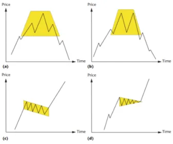
analysis of diagrams that show the changes of price over time. The important at-tributes of these charts are: Opening and closing price, maximum and minimum price for a specified period of trading time and etc [17]. Variation of price over time that is usually used by technical analysts is shown in Fig. 2.1.
Figure 2.1:Visual analysis
• Auditory displays: These try to extract valuable information from sound by con-sidering pitch and volume.In [18], author extended his audification techniques (representing a sequence of data values as sound signal) for making a sound display by converting stock market price data into a sound waveform (and then be able to process it with sound processing techniques). Nevertheless, author concludes that it was not easy to interpret such kind of sound waveforms.
2.2
Depth of Market Data
The visual displays that mentioned above let the traders to find and recognize patterns in charts. But most of the time these charts cover variations in a period of a day. For making better decisions, each transaction can be charted minute by minute and then a trader can extract valuable information from it [19].
Moreover, traders might take advantage of information prepared by the market’s depth. The Depth of market is the number of buyers and sellers in each minute of a day, trying to trade in stock market [19]. A buyer might make a bid to purchase a speci-fied volume of shares while at the same time a seller might ask a price for some specispeci-fied volume. The balance of bids and asks determines the current market state.
One of the advantages of depth of market is order imbalance. Order imbalance is a situation resulting from an excess of buy or sell orders for a specific stock, making it im-possible to match the buyers and sellers orders [20]. In next subsection we will talk about it in more details.
2.3
Order Imbalance (OI)
Up to now, many studies have been tried to explain the relationship between trade vol-ume (or number) and price variations during that period and dispersion of returns of each stock called as volatility. When the traders start to register their buy (sell), at the same time they affect bid (ask) volumes and price of each stock. In this part we can un-derstand the traders intentions and the prices changes consequently. Order imbalances is the quantification of these intentions. In the other word order imbalance is the way to show the difference between buy and sell orders. Chordia and Subrahmanyam [21], using the sample from New York stock market, showed that the relationship between order imbalance and daily return is positive. So it can be said that Order imbalance is an important concept for understanding traders intentions and market’s direction [1]. If some traders have specific prior information (which other traders do not have), where the information has not been applied to asset price yet, considering being aware of that
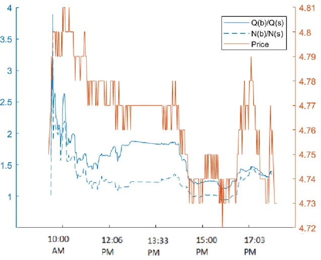
triggering of market crashes of ISBANK stock. The Blue dotted graph presents the
num-ber order imbalance changes (Number of buy ordersNumber of sell orders = NB
NS), and the blue solid graph is the
quantity order imbalance changes (Quantity of buy ordersQuantity of sell orders = QB
QS) during 9:35 AM to 5:30 PM
(the left axis vs time on horizontal axis). Also the red solid graph is showing the price changes on the date 30/11/2015 (the right axis vs time on horizontal axis).
Figure 2.2:The blue dotted line and blue solid line are respectivelyNb
Ns and
Qb
Qs (left axis)
versus time and the red solid one (right axis) is price versus time on the date 30/11/2015, for ISBANK stock.
2.3.1
Number and Quantity based Order Imbalances
In this part we are going to explain about order imbalances that we use in this thesis. The definition that are used for order imbalances are as follows:
OIt ,1N = NB− NS (2.1)
OIt ,1Q = QB−QS (2.2)
where,
NB:Number of buying orders (2.3)
NS:Number of selling orders (2.4)
QB:Quantity of buying orders (2.5)
QS:Quantity of buying orders (2.6)
Another measure for order imbalance, that we are going to use are
OIt ,2N =NB
NS (2.7)
OIt ,2Q =QB
QS (2.8)
Another important point that we should mention is that, The OIs that considered above only measures the magnitude of the imbalance which is not sufficient to describe the behavior of the traders in the market. For example using the order imbalance Eq. 2.1,
OIQt ,3=QB−QS
QB+QS (2.10)
Another equation that is used in this study with data analytics is the percentage
changeof OIs in each minute:
∆OIN t = OItN− OI(t −1)N OI(t −1)N (2.11) ∆OIQ t = OIQt − OIQ(t −1) OIQ(t −1) (2.12)
2.4
Order Flow Imbalance (OFI)
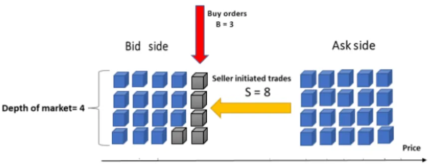
In 2014 cont et al. [24] introduced order flow imbalance (OFI), as a variable that accu-mulates the sizes of orders, and omits cancel orders to make a balance between supply and chain at the best bid and ask price. Although order flow imbalance can support im-portant evidence for a linear relation between price variation, and OFI in stock markets. The OFI process tracks best bid and ask queues and change much faster than prices [25]. In the Fig. 2.3, Fig. 2.4 and Fig. 2.5, the order flow imbalance is illustrated with a simple example. Assume that the depth of market is four in each side (blue color). The seller initiated trades and cancellation (refer to Chapter1 section 1.2), totally remove ten stock from the bid side (gray color). Also at the same time new buy orders add three stock again to the bid side.
Figure 2.4:Adding new buy orders to the bid side
Figure 2.5:Removing buy cancellation from bid side
2.4.1
Number and Quantity based Order Flow Imbalances
The Eq. 2.13 to Eq. 2.16 and Eq. 2.17 to Eq. 2.22 are shown below for calculation of OFIs in this thesis.
BN=Number of arrived buy orders− Number of cancelled buy orders
SQ=Quantity of arrived sell orders− Quantity of cancelled sell orders
−Quantity of buyer initiated trades (2.16)
OF It ,1N = NB− NS (2.17) OF It ,1Q = QB−QS (2.18) OF It ,2N =NB NS (2.19) OF IQt ,2=QB QS (2.20) OF It ,3N =NB− NS NB+ NS (2.21) OF It ,3Q =QB−QS QB+QS (2.22)
The percentage change of OFIs will be calculated using Eq. 2.23 and Eq. 2.24:
∆OF IN t = OF ItN− OF I(t −1)N OF It −1N (2.23) ∆OF IQ t = OF IQt − OF I(t −1)Q OF IQt −1 (2.24)
Chapter 3
Quantitative Statistics
3.1
Literature Review
In literature, starting with definition of high frequency trading, HFT has been the subject of intense public debate and discussions. HFT or more traditional, "Quantitative Invest-ing", have a huge impact on markets by producing efficient algorithm to make accurate decisions. Generally HFT concentrates more on the information that price movements might transfer about the trading strategies or signals of other markets [2, 4].
S. LaValle et al. [26], do a research on about 3000 company and businesses and show that big data can be the most reliable tool in making precise decisions in financial mar-kets. Also the successful companies use data analytics based on big data five times more than others.
order imbalances in NYSE data sets of eleven years. They showed that there is positive au-tocorrelation in daily order imbalances and also they have negative relation with monthly returns.
Lee et al. [29], showed the relationship between order imbalances and market effi-ciency in the "Taiwan Stock Exchange". The accessible data include all orders submitted to the Taiwan Stock Exchange (TWSE) from September 1996 to April 1999. They find that domestic institutions have more stable and reliable order imbalances in comparison to large companies. Also, The major orders of large individual investors had weak perfor-mance, that showed these agents act like noise traders. Although, the orders of domestic institutions have low price impact and also profitable.
Using Taiwanese stocks from 1994 to 2002, Andrade et al. [30], apply regression analy-sis and a sorting procedure to study the foreseeable return of price implied by the multi-asset equilibrium model. As a result they showed that stocks with more delicate order imbalances have more volatile returns.
Kaniel et al. [31], focus on the interaction between individual investors and stock re-turns. They examined the short-horizon dynamic relation between the buying and sell-ing by individuals and both previous and subsequent returns ussell-ing a unique data set provided by the New York Stock Exchange (NYSE) from 2000 to 2003. Their work suggests that understanding the behavior of one investor type, individuals, holds some promise for explaining observed return patterns.
Cont et al. [24], introduced order flow imbalance as the imbalance between supply and demand at the best bid and ask prices. They showed that there is a linear relation between order flow imbalance and price variation. The slope of this relationship is in-versely proportional to the market depth. Also their results were robust to daily season-ality effects, and persistent across time scales and across stocks.
Hanke et al. [32], investigated effects of order flow imbalance on daily returns of Ger-man stocks. They used fixed-effects panel regressions instead of time series analysis. For the conditional relation (including concurrent order imbalance), their results confirm
those of previous studies. For the unconditional relation (which allows forecasting re-turns from past order imbalance), the results were qualitatively in line with the literature, but the effects were weaker.
Michael Goldstein et al. [33], showed that order imbalances are strong predictors of future prices in ASX (Australian Securities Exchange). At the same time, when the order imbalance moves in an unfavourable direction, they are quick to cancel or amend orders that are at high risk of being picked off by other traders.
Finally, our work is the extension of master thesis “Order imbalanced based strategy in high frequency trading” by Darryl Shen, [1]. Firstly they introduced the area of high frequency trading and the data that will be used to test the trading strategy. Then they extended a simple trading strategy with fitting a linear model between average price re-turns and order imbalances to see if the model can predict the return properly or not?. They showed that the mentioned strategy in the article, using this linear model to fore-cast future price changes is profitable when, the forefore-cast is greater than 0.2.
In this thesis our analysis is based on useful information of benchmark index BIST 30. During our sample period (30th of November 2015 till end of April 2016), 27 out of 30 stocks are all included in the benchmark index. We focus on these 27 stocks because we do not want to be affected by inclusion\exclusion in\from the index. We make use of a long time series of transaction level data from the Borsa Istanbul database for answering the two questions. Firstly whether data analytics based on order imbalances and order flow imbalances can predict individual future returns (time series analysis)?. Secondly, we are trying to find out the prediction power of data analytics using cross sectional anal-ysis like Fama-Macbeth regression and long short portfolio.
3.2
The Borsa Istanbul
The Istanbul Stock Exchange (ISE), was founded as an autonomous, professional orga-nization for the unique exchange unit in Turkey in early 1986. Then the borsa istanbul (abbreviated as BIST) was founded on the December 30, 2012, for starting a modern stock market [34] and gathered all the exchanges operating in the Turkish capital markets to-gether in the same place. Required documents of staring was provided by the capital markets board, and then approved by minister in charge. Formally, it was registered on April 3, 2013, and received operation permit.
The main goal of Borsa Istanbul is that, With observing the law and legislation, let to all kind of stock exchanges like foreign currencies, valuable metals, and contracts, im-portant documents, and assets approved by the capital markets board of Turkey to trade in a free, secure and stable circumstances [34, 35].
3.2.1
Structure of Data
As one of the world’s top ten biggest emerging markets, BIST successfully has absorbed considerable foreign investment. By 2015-May, average daily trade volume was 4.4 bil-lion Turkish Lira ($1.6 bilbil-lion dollar) for around 420 listed stocks in the market [35]. The time period of this study is from 2015-November-30 to 2016-April-30 which contains 109 trading days.
Additional explanation about trading mechanisms and rules in BIST is helpful to have better understanding of AT and HFT involvement in the market. First, this should be noted that stocks of all publicly held companies in BIST, are exclusively traded, showing no market fragmentation. On the other hand, HFT strategies which are seen in BIST are most likely more diverse, leading to higher number of HFT (for instance, HF arbitrage strategies among different markets). Except those in watch list, short selling (is an trading strategy that is based on the decline in a stock price and selling it before declination.) is available for all listed stocks. In our analyses, stocks are limited to those in BIST 30 index list which can be sold short.
In BIST, trading time interval in every work day (Monday to Friday) is from 9:35 AM to 12:30 PM, and from 13:30 PM to 17:30 PM continuously. There are three call auction steps. Prices are fixed at 09:30 AM, 13:55 PM, and 17:35 PM (orders are collected from 09:15 to 09:30, from 13:00 to 13:55 and from 17:30 to 17:35), which after that, trading goes on at closing price until 17:40 PM. For our examined time period from 2015-November-30th to 2016-April-30, trading takes place within two sessions (morning and afternoon). Overall, trading mechanism is pretty similar. Both trading sessions start with single price call auctions followed by continuous auctions. At the start of our study period, first (sec-ond) session’s call auction takes place between 09:30 AM and 9:50 AM (14:00 PM and 14:15 PM). Continuous auction for first (second) session is between 09:50 AM and 12:30 PM (13:30 PM and 17:30 PM). Closing call auction takes place between 17:30 PM and 17:40 PM.
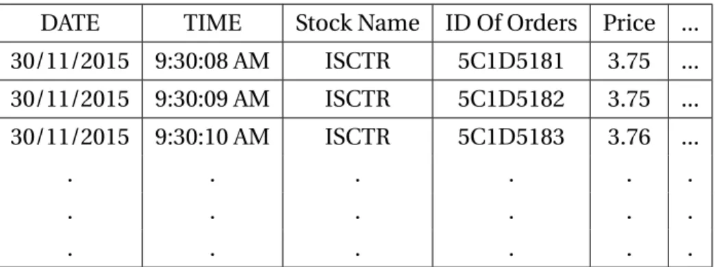
The data is arranged in two tables. Table 3.1 contains the information of stocks in each day like, date, time, ID number of order, price and, etc.
Table 3.1:Sample data set for ISCTR, on date 2015/11/30.
DATE TIME Stock Name ID Of Orders Price ...
30/11/2015 9:30:08 AM ISCTR 5C1D5181 3.75 ... 30/11/2015 9:30:09 AM ISCTR 5C1D5182 3.75 ... 30/11/2015 9:30:10 AM ISCTR 5C1D5183 3.76 ... . . . . . . . . . . . .
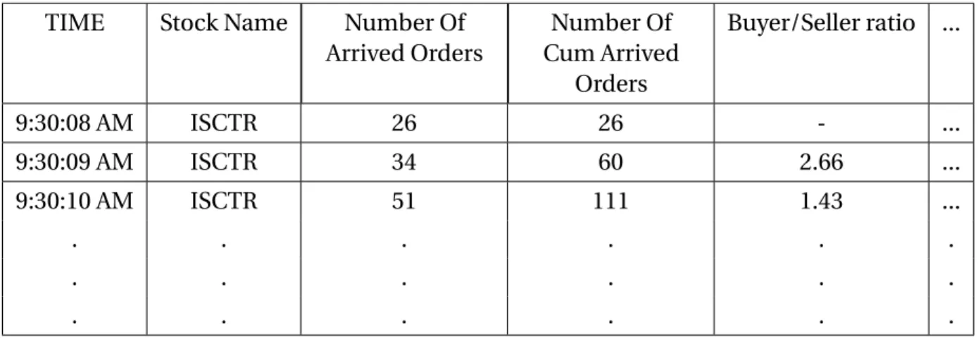
The second table 3.2 includes, time, number of arrived orders, cumulative number of arrived orders, quantity of arrived orders, cumulative quantity of arrived orders, etc.
Table 3.2:Sample data set for ISCTR, on date 2015/11/30, starting hour 9:30 AM.
TIME Stock Name Number Of
Arrived Orders Cum ArrivedNumber Of
Orders Buyer/Seller ratio ... 9:30:08 AM ISCTR 26 26 - ... 9:30:09 AM ISCTR 34 60 2.66 ... 9:30:10 AM ISCTR 51 111 1.43 ... . . . . . . . . . . . .
The data analytics which is used here is published by Borsa Istanbul on first of June, 2016. These critical analytics are usable by traders, market makers and etc. The data analytics are calculated per 60 seconds and include following categories:
• Order arrival analytics: Number \Quantity of orders arriving per 60 seconds. • Order cancellation analytics: Number \Quantity of cancelled buy \sell orders per
60 seconds
• Volume weighted average price analytics: Is a trading benchmark used by traders that gives the average price a stock has traded at throughout the day, based on both volume and price.
• Buyer-seller analytics: Data analytics which can result from buy and sell orders. We use all above analytics except of, volume weighted average price analytics, in this thesis.
3.3
Data Statistics
In this section, the result of statistics for all data set is presented. The Table 3.3 includes total number of buy and sell for each company, total quantity of buy and sell for each company, average of one minute return in 109 days and their standard deviation for all 27 companies.
C ompany Name T otal number of buy or ders T otal number of sell or ders T otal quantity of buy or ders T otal quantity of sell or ders A vg 1-min R etur n 109 D ay S tandar d D eviation of 1-min R etur n AR CLK 196457 174727 203306566 210897707 -0.00019 0.00077 BIMAS 157744 144005 100607405 102121629 -0.00024 0.00055 DO AS 225710 185614 189983193 196637008 -0.00004 0.00070 ENK AI 119709 115091 328278623 202091455 0.00008 0.00130 EREGL 253459 226533 1692718944 2047067813 -0.00007 0.00131 FR O T O 144118 141268 45795997 47736261 0.00013 0.00104 GARAN 901913 901872 12731457320 12478018844 0.00001 0.00084 HALKB 681741 619802 3244629128 3346063766 -0.00045 0.00064 ISCTR 532339 454827 4777386480 5182552252 -0.00009 0.00113 K CHOL 280363 228415 447198542 446852288 0.00027 0.00075 K OZ AL 342373 296349 126246448 134429175 0.00009 0.00104 KRDMD 313522 247440 5360780379 4412047814 0.00038 0.00344 O TK AR 191792 160490 25079021 25044383 -0.00003 0.00074 P ETKM 219822 167853 1401413338 1495274124 0.00063 0.00115 PGSUS 268030 231209 185833359 190003901 -0.00062 0.00048 SAHOL 270933 238693 1222313452 1194185499 0.00008 0.00065 SISE 146587 146885 561210981 651752702 0.00028 0.00139 T A VHL 284126 239309 199873002 203015356 -0.00080 0.00068 T CELL 253086 229562 443080962 470889479 0.00009 0.00068 THY A O 1007486 978144 7121278038 8146725500 -0.00064 0.00094 TKFEN 166782 147041 656534724 655330440 0.00042 0.00091 T O ASO 204447 190100 156869873 153210255 0.00008 0.00093 T TK OM 155703 158450 418012555 418840477 -0.00015 0.00089 TUPRS 356191 304683 178196683 175590983 -0.00002 0.00053 ULKER 20217 18725 14166608 13288852 -0.00003 0.00066 V AKBN 27429 25487 875263419 65874122 0.00009 0.00078 YKBNK 478530 428531 1187238693 1222317852 0.00003 0.00085 T able 3.3: Selected statistics of 27 companies stocks fr om 30th of N ov ember 2015 till the end of Apr il 2016.
Chapter 4
Time Series Analysis
In this chapter, we aim to improve the existing strategy of generating profit by extending the linear models with new factors and, also by optimizing the regression and trading parameters. The improvements described in this section, enhance the profit value con-siderably. In the first section, we explain the time series analysis briefly. After that, we introduce new factors related to order imbalances. Then, we estimate the coefficients and number of significant days. Finally, in the last part, order flow imbalances and the regression models by new factors are discussed.
4.1
Time Series in Finance
Generally, continuously monitoring the price behavior to realize the probable change of the price in the future is desirable. Due to this, deeper understanding of price behavior
There are two major goals to study and investigate financial time series [36]. First is importance of realizing price behavior. In this case, the variance of time series is specially relevant. Tomorrow’s price is uncertain and then, it should be explained with probability distribution. Therefore, statistical methods are normal ways to investigate price behav-ior. Usually a model is designed that describes of how successive prices are determined in details. The second goal is to use our knowledge of price behavior to decrease risk and take more suitable decisions. Typically, time series models are applicable in forecasting, risk management, and option pricing.
4.1.1
Stationarity in Time Series
High Frequency Trading and applications of their strategies are closely related to the ergodic theory of stationary processes. We explain two kind of stationary. A
time-series Xt is strongly stationary if (Xt 1, Xt 2, ..., Xt n) has the same distribution as
(Xt 1+a, Xt 2+a, ..., Xt n+a)for alla and any arbitrary integern > 0. Another stationary
defi-nition for the time-seriesXt, is weakly stationary, that is, if the first two moments do not
change over time, or in another words,E [Xt] = E[Xt +a] = µandC ov(Xt; Xt +a) = afor all
timetand arbitrarya. It is sufficient for the data to be weak stationary for traders to build
an algorithmic trading strategy which generates positive expected profit.
Further theory regarding stationary processes, the strong ergodic theorem, and its ap-plicability in high frequency trading can be found in [36]. One of the important tests in proving stationary in time series is KPSS (Kwiatkowski–Phillips–Schmidt–Shin) test (re-fer to [37] for more information). The usage of KPSS is testing a null hypothesis that an observable time series is stationary around a deterministic trend, against the alternative of a unit root (not to be stationary).
In this thesis, we apply KPSS on all of our variables that we want to use in regression models as predictor variable. For forecasting, we absolutely need to find the constant (time invariant) component in the series, otherwise it’s impossible to forecast by defini-tion. Stationarity is just a particular case of the invariance.
to reject the trend-stationary null and one indicates rejection of the trend-stationary null in favor of the unit root alternative. Also two other outputs are p value and t statistics. We define all variables including order imbalances and percentage changes in Eq. 2.1 to Eq. 2.12 and Eq. 2.17 to Eq. 2.24 respectively. According to t stats and p values, all of the variables are stationary. Instead of h values table, that all of them are one, the Tables 4.1 and 4.2 include t stats of KPSS test in the fifth lag (up to five lag of time, stationary has been checked) for all variables on 30th of November for all 27 companies.
C ompany Name OI N t,1 O I Q t,1 OI N t,2 OI Q t,2 OI N t,3 OI Q t,3 ∆ O I N t,1 ∆ OI Q t,1 ∆ O I N t,2 ∆ OI Q t,2 ∆ OI N t,3 ∆ OI Q t,3 AR CLK 0.16240 0.14468 0.15714 0.18041 0.33563 0.26000 0.18816 0.07940 0.15608 0.07035 0.04746 0.04367 BIMAS 0.20456 0.09362 0.10673 0.07899 0.32341 0.27845 0.04500 0.07580 0.11480 0.05379 0.05157 0.04849 DO AS 0.12943 0.08765 0.08756 0.10364 0.27870 0.26980 0.05176 0.09090 0.11104 0.10662 0.05610 0.10954 ENK AI 0.12291 0.08767 0.11549 0.26579 0.72109 0.63102 0.21438 0.06715 0.14849 0.09046 0.12953 0.04910 EREGL 0.19821 0.13220 0.17864 0.18153 0.60189 0.48076 0.06667 0.15175 0.15568 0.40467 0.07870 0.02948 FR O T O 0.11689 0.19481 0.14960 0.30300 0.41930 0.33732 0.07753 0.01274 0.14828 0.59796 0.05069 0.06113 GARAN 0.20880 0.06844 0.09854 0.10688 0.45135 0.15476 0.03742 0.05642 0.07935 0.22563 0.12000 0.25913 HALKB 0.08423 0.05164 0.15726 0.16970 0.59522 0.45370 0.07340 0.08839 0.23274 0.18901 0.66681 0.30953 ISCTR 0.10128 0.87408 0.17579 0.17565 0.33372 0.37083 0.25969 0.03530 0.11314 0.19904 0.10523 0.04663 K CHOL 0.07647 0.08376 0.10783 0.08283 0.66023 0.63680 0.10999 0.02672 0.10913 0.04357 0.08510 0.11451 K OZ AL 0.20543 0.14614 0.15610 0.19146 0.45212 0.42236 0.20073 0.04062 0.15753 0.20993 0.14650 0.03215 KRDMD 0.04808 0.13625 0.13541 0.07574 0.13784 0.34586 0.76075 0.08137 0.10940 0.10729 0.14768 0.05966 O TK AR 0.07808 0.32256 0.12525 0.13488 0.06666 0.05793 0.37704 0.10952 0.09900 0.08879 0.10849 0.10077 P ETKM 0.12393 0.13676 0.16345 0.03694 0.26299 0.21680 0.05276 0.07707 0.15182 0.63337 0.07632 0.02785 PGSUS 0.14668 0.12180 0.15596 0.08039 0.10508 0.21861 0.27830 0.04593 0.12905 0.06788 0.38003 0.05834 SAHOL 0.11238 0.07568 0.18628 0.17493 0.43147 0.35581 0.09458 0.04816 0.14730 0.17944 0.04459 0.06616 SISE 0.14454 0.10087 0.18818 0.04066 0.52867 0.62483 0.52330 0.04806 0.12684 0.04247 0.16115 0.04590 T A VHL 0.16952 0.09342 0.12075 0.03565 0.26275 0.27259 0.09740 0.05521 0.11428 0.03671 0.04803 0.05243 T CELL 0.13851 0.06819 0.49767 0.72001 0.43228 0.40911 0.09160 0.04332 0.38457 0.42461 0.05820 0.78360 THY A O 0.30495 0.07955 0.22851 0.33228 0.34134 0.42579 0.09366 0.04255 0.28034 0.05945 0.05310 0.04324 TKFEN 0.19531 0.12582 0.12268 0.04900 0.13351 0.40260 0.16343 0.11860 0.12930 0.03306 0.10592 0.06679 T O ASO 0.18858 0.04321 0.29832 0.32433 0.36841 0.38266 0.13822 0.07257 0.16654 0.37838 0.40685 0.06218 T TK OM 0.49093 0.10045 0.18193 0.26538 0.30223 0.33204 0.28566 0.06287 0.13045 0.75055 0.06896 0.08972 TUPRS 0.14499 0.03872 0.10470 0.19184 0.24973 0.44323 0.34866 0.11367 0.17673 0.08371 0.05875 0.03105 ULKER 0.11321 0.09876 0.11998 0.11759 0.48464 0.50114 0.29104 0.09672 0.12387 0.03634 0.03846 0.10162 V AKBN 0.06873 0.07973 0.16537 0.08574 0.31059 0.29222 0.03624 0.05765 0.16549 0.07389 0.08165 0.08274 T able 4. 1: tstats of KPSS test of all var iable sincluding or der imbalances and their per centage changes which ar e defined in Eq .2.1 to Eq .2.12, on the date 30/11/2015 for all companies .
OF I Q t,1 O FI N t,2 OF I Q t,2 O FI N t,3 OF I Q t,3 ∆ OF I N t,1 ∆ OF I Q t,1 ∆ OF I N t,2 ∆ O FI Q t,2 ∆ OF I N t,3 ∆ O FI Q t,3 0.04621 0.10680 0.10699 0.15901 0.06694 0.12358 0.04343 0.08728 0.07126 0.25677 0.04896 0.04227 0.10126 0.05790 0.10884 0.07084 0.66626 0.07465 0.03600 0.08633 0.05201 0.03287 0.06720 0.08553 0.06287 0.10833 0.10083 0.12074 0.10869 0.06201 0.05164 0.10975 0.05505 0.07042 0.15815 0.08009 0.38400 0.19212 0.06452 0.06994 0.08629 0.05940 0.04803 0.03760 0.06946 0.09057 0.02788 0.15815 0.05166 0.06380 0.03634 0.05317 0.07841 0.12531 0.06356 0.11705 0.07128 0.07995 0.09702 0.05152 0.08796 0.06885 0.06896 0.04384 0.09138 0.03593 0.05117 0.03384 0.08360 0.04040 0.07412 0.02490 0.05080 0.05935 0.05218 0.09640 0.05895 0.04908 0.15640 0.07165 0.24832 0.09125 0.04842 0.04158 0.09531 0.04505 0.05995 0.06180 0.05065 0.07416 0.10274 0.17357 0.12546 0.07407 0.03803 0.10097 0.08189 0.09205 0.05368 0.07147 0.03603 0.04117 0.08298 0.05546 0.27832 0.06425 0.06572 0.05105 0.10675 0.02971 0.06783 0.16937 0.04155 0.15594 0.14535 0.18147 0.06555 0.14301 0.12642 0.05176 0.14359 0.09601 0.04298 0.04739 0.30483 0.04872 0.06359 0.10943 0.07425 0.04505 0.05977 0.03604 0.12579 0.15769 0.14706 0.45032 0.08315 0.23014 0.09429 0.08769 0.04695 0.07895 0.08436 0.06185 0.24745 0.07381 0.48269 0.10109 0.07308 0.09882 0.15893 0.09337 0.09975 0.11248 0.06920 0.18543 0.03014 0.40089 0.04094 0.05859 0.07435 0.07043 0.03461 0.02614 0.05805 0.04475 0.07146 0.07977 0.04338 0.05981 0.06074 0.03926 0.09754 0.02606 0.02020 0.07665 0.08550 0.07049 0.05701 0.07626 0.04648 0.14734 0.04548 0.05124 0.09201 0.06765 0.04537 0.05730 0.11735 0.05977 0.08274 0.06830 0.07406 0.06483 0.04834 0.02122 0.04488 0.06439 0.08534 0.18668 0.13583 0.13555 0.15684 0.18318 0.03206 0.04888 0.08260 0.06303 0.07328 0.05104 0.05514 0.07160 0.06226 0.06903 0.07090 0.05293 0.17573 0.05228 0.07806 0.14729 0.11300 0.09112 0.12960 0.47247 0.46843 0.16087 0.07939 0.05554 0.03594 0.10626 0.14319 0.06656 0.13465 0.17382 0.30730 0.03720 0.07718 0.03910 0.10953 0.14397 0.07967 0.08070 0.13251 0.22822 0.06154 0.34425 0.19413 0.26118 0.04952 0.07897 0.05036 0.05521 0.04589 0.03444 0.08077 0.06038 0.14124 0.05095 0.40868 0.02907 0.06169 0.04437 0.04226 0.06630 0.14672 0.27048 0.04422 0.27557 0.12842 0.06267 0.03573 0.12043 0.04541 0.05212 0.07092 0.05392 0.07159 0.09068 0.14722 0.07283 0.06584 0.03175 0.04531 0.09694 0.03357 0.08527 test of all var iables including or der flo w imbalances and their per centage changes which ar e defined on the date 30/11/2015 for all companies .
4.1.2
Autocorrelation and Cross Correlation of Order Imbalances
Autocorrelation is a mathematical representation of the degree of similarity between a given time series and a lagged version of itself over successive time intervals. It is the same as calculating the correlation between two different time series, except that the same time series is actually used twice, once in its original form and once lagged one or more time periods.
Order imbalance has positive autocorrelation as presented in Fig. 4.1 for most days, the order imbalance autocorrelation is significant up to lag 15. This indicates that pos-itive imbalances are often followed by periods of persistent pospos-itive imbalances due to traders splitting their orders across multiple periods, as explained by Chordia [28]. On the other hand, other studies argue that this phenomenon is caused by herding among investors.
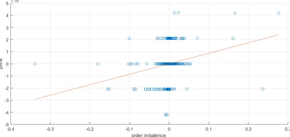
We also show that the order imbalance is positively correlated with contemporary price changes. The below figures (Fig. 4.2 and Fig. 4.3) illustrate this positive relationship.
Figure 4.1:Autocorrelation ofOIt ,2N =NB
NS on the date 30/11/2015, for ISBANK stock.
Figure 4.2:Cross correlation of price return
andOIt ,2N = NB
NS on the date 30/11/2015, for
ISBANK stock.
Figure 4.3: Scatter plot ofOIt ,2N = NB
NS versus contemporary price changes on the date
4.2
Order Imbalance-based Models
We propose some linear and nonlinear models where we predict future price change with the current (instantaneous) and lagged OIs. Chordia [28], Huang [23], and Cont [24] all build linear models with lagged order imbalances as the explanatory variable and the immediate one-period price change as the response. We also make the assumption that
the errors²t are independent and normally distributed with zero mean and constant
variance.
4.2.1
Models with Percentage Changes (
∆
)
We present some statistical properties of the explanatory and response variables before analyzing the linear model. We define percentage return for 1 minute ahead (t+1) with Eq. 4.1 and we use it as the response variable.
rt +1=pr i cet +1− pr i cet
pr i cet (4.1)
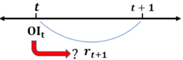
The Fig. 4.4 shows the basis of constructing models for ability of prediction of 1-min
ahead return, using∆OIt.
Figure 4.4:Power of prediction of∆OIt in 1-minute ahead return
According to above Eq. 4.1 as response variable, the first models are,
rt +1= β0+ β1∆OItN+ ²t +1 (4.2)
The second models are,
rt +1= β0+ β1∆OItN+ β2rt+ ²t +1 (4.4)
rt +1= β0+ β1∆OItQ+ β2rt+ ²t +1 (4.5)
Wherert is the lagged return of price. Also the third models listed as below,
rt +1= β0+ β1∆OItN+ 4 X j =0 βj +2rt −j+ ²t +1 (4.6) rt +1= β0+ β1∆OItQ+ 4 X j =0 βj +2rt −j+ ²t +1 (4.7)
In addition to three linear models that have been proposed in previous section, an-other new model is introduced. The nonlinear fourth models are as follows:
rt +1= β0+ β1∆OItN+ β2∆OItN|∆OItN| + ²t +1 (4.8)
rt +1= β0+ β1∆OIQt + β2∆OItQ|∆OI Q
t | + ²t +1 (4.9)
These models are estimated independently using the data set of Borsa Istanbul for each of the 109 trading days (30/12/2015 to 29/04/2016), using ordinary least squares
linear regression. We use allOIt ,1N ,OIQt ,1,OIt ,2N ,OIt ,2Q ,OIt ,3N andOIQt ,3as explanatory
vari-ables in all four models that was introduced in Eq. 4.2 to Eq. 4.9 .
In the time-series regression, we first drive information of 27 stocks on the basis of or-der imbalances and their percentage changes and also the return of each minute. There
In the model 4.10, TAVHL has 105 significant days out of 109 positive days with aver-ageR2= 0.031.
rt +1= β0+ β1∆OIt ,2N + β2rt+ ²t +1 (4.11)
In the model 4.11, PGSUS with 101 significant days and ENKAI, TAVHL , TUPRS with 100 significant days out of 109 positive days are the best ones.
rt +1= β0+ β1∆OIt ,3N +
4
X
j =0
βj +2rt −j+ ²t +1 (4.12)
In the model 4.12, PGSUS has 100 significant days out of 109 positive days with
av-erageR2= 0.06296.
rt +1= β0+ β1∆OIt ,2N + β2∆OIt ,2N |∆OIt ,2N | + ²t +1 (4.13)
In the model 4.13, we have the strongest results between all. for example HALKB has
109 significant positive days out of 109 days withR2= 0.06548.
Moreover∆OIN
t ,2 whichOIt ,2N =
NB
NS represents the strongest factor in explaining the
Turkish stock returns and showing strong association with price return in all 27 stocks.
In the Tables 4.3 to 4.17, the average of estimated coefficients and adjustedR2and
number of positive days (estimated coefficient of day is positive) are depicted. Also an-other important calculated parameter is the number of significant days that significant level is 0.05 here. It means that in that days p value is less than 0.05.
rt+ 1 = β0 + β1 ∆ OI N t,1 + ²t+ 1 rt+ 1 = β0 + β1 ∆ O I Q t,1 + ²t+ 1 A vg of β1 # of P ositiv e β1 # of S ig P ositiv e β1 A vg of R 2 A vg of β1 # of P ositiv e β1 # of S ig P ositiv e β1 1.95E-06 60 7 0.00060 -1.10E-08 51 4 9.81E-06 50 15 0.00002 4.86E-08 59 4 1.20E-06 55 10 0.00055 4.11E-09 60 6 -1.90E-06 55 6 0.00327 2.57E-08 58 11 5.22E-06 66 8 0.00076 7.22E-09 65 2 4.28E-06 58 7 0.00140 -3.17E-08 59 7 1.51E-06 70 4 -0.00039 -1.04E-09 48 4 9.75E-07 62 5 -0.00055 2.20E-08 58 1 2.23E-06 63 7 0.00012 -9.16E-09 52 2 2.10E-06 66 5 -0.00019 1.46E-08 67 2 3.45E-06 59 6 0.00007 -3.01E-08 59 4 4.47E-06 62 6 0.00046 -4.91E-09 49 6 5.76E-06 71 9 0.00208 4.59E-07 70 13 2.09E-06 62 4 0.00178 1.89E-08 56 11 2.04E-07 55 5 -0.00046 1.74E-08 63 2 -4.75E-07 59 5 -0.00013 2.46E-09 55 3 1.00E-05 64 7 0.00121 7.98E-09 58 6 -5.86E-07 49 7 0.00018 -9.87E-09 49 4 4.75E-07 54 4 -0.00010 -4.66E-09 52 1 -1.15E-07 51 3 -0.00033 1.17E-08 54 1 1.52E-06 52 6 0.00156 -3.56E-10 49 5 2.35E-06 51 9 0.00091 -2.65E-08 46 7 -6.58E-06 35 1 0.00111 -6.48E-09 44 6 1.34E-06 59 3 -0.00106 -2.16E-08 50 0 -2.60E-06 51 8 0.00308 -4.94E-08 58 8 3.55E-06 69 8 0.00051 -7.34E-09 57 5 1.74E-06 60 8 0.00017 -4.96E-10 61 4 first model using per centage changes of O I N t,1 = NB − NS and O I Q t,1 = QB − QS for 27 companies since