RESONANT OPTICAL NANOANTENNAS AND
APPLICATIONS
a thesis
submitted to the program of material science and
nanotechnology
and the institute of engineering and sciences
of bilkent university
in partial fulfillment of the requirements
for the degree of
master of science
By
Murat Celal KILINC
¸
August 2010
I certify that I have read this thesis and that in my opinion it is fully adequate, in scope and in quality, as a thesis for the degree of Master of Science.
Assist Prof. Dr. Mehmet Bayındır (Supervisor)
I certify that I have read this thesis and that in my opinion it is fully adequate, in scope and in quality, as a thesis for the degree of Master of Science.
Assist Prof. Dr. Ali Kemal Okyay
I certify that I have read this thesis and that in my opinion it is fully adequate, in scope and in quality, as a thesis for the degree of Master of Science.
Assist Prof. Dr. Sel¸cuk Akt¨urk
Approved for the Institute of Engineering and Sciences:
Prof. Dr. Levent Onural
ABSTRACT
RESONANT OPTICAL NANOANTENNAS AND
APPLICATIONS
Murat Celal KILINC
¸
M.S. in Material Science and Nanotechnology
Supervisor: Assist Prof. Dr. Mehmet Bayındır
August 2010
Being one of the fundamentals of electrical engineering, an antenna is a metal-lic shape structured to transmit or receive electromagnetic waves. Thanks to the recent advances in nano fabrication and nano imaging, metallic structures can be defined with sizes smaller to that of visible light, wavelengths of several nanometers. This opens up the possibility of the engineering of antennas working at optical wavelengths. Nanoantennas could be thought of optical wavelength equivalent of common antennas. Today physics, chemistry, material science and biology use optical nanoantennas to control light waves. Optical nanoantennas are tailored for many technological applications that include generation, manip-ulation and detection of light. The near field enhancement of resonant optical nanoantennas at specific wavelengths is their most promising advantage that attracts technological applications. In this thesis, we study the resonance char-acteristics of optical nanoantennas and investigate the governing factors by nu-merical calculations. We also evaluate radiated electric field from the resonating nanoantenna. Finally, we employ the resonant near field enhancement in optical
nonlinear generation. The fabrication of nanoantennas with FIB milling is also explored.
¨
OZET
OPT˙IK DALGA BOYLARINDA C
¸ ALIS¸AN, REZONE EDEN
NANOANTENLER VE UYGULAMALARI
Murat Celal KILINC
¸
Malzeme Bilimi ve Nanoteknoloji B¨ol¨
um¨
u Y¨
uksek Lisans
Tez Y¨oneticisi: Yar. Do¸c. Dr. Mehmet Bayındır
A˘gustos 2010
Elektrik m¨uhendisli˘ginin temel yapıta¸slarından olan antenler elektromanyetik dalgaları yaymak ve almak i¸cin tasarlanmı¸s metal ¸sekillerdir. Nano fabrikasyon ve nano boyutta g¨or¨unt¨uleme tekniklerinin geli¸smesi ile birlikte metal ¸sekillerin g¨or¨un¨ur ı¸sı˘gın dalgoboyundan k¨u¸c¨uk boyutlarda, nano boyutlarda, dahi fabrike edilmesi m¨umk¨un hale gelmi¸stir. Nano boyutlu metal ¸sekiller sayesinde op-tik dalga boylarında ¸calı¸san antenlerin m¨uhendisli˘ginin ¨on¨u a¸cılmı¸stır. Nano antenler radyo antenlerinin optik dalga boylarında ¸calı¸san e¸sde˘geri sayılabilir. Bug¨un, fizik, kimya, malzeme bilimi ve biyoloji nanoantenleri ı¸sık dalgalarını kontrol etmek i¸cin kullanmaya ba¸slamı¸stır. Nanoantenler ı¸sı˘gın ¨uretiminin, manip¨ulasyonunun ve algılanmasının yer aldı˘gı teknolojik uygulamalar i¸cin d¨uzenlenmektedirler. Optik nanoantenlerin rezone ettikleri dalga boyları i¸cin, y¨uzeylerinde ve y¨uzeylerine yakın yerlerde, dikkat ¸ceken elektrik alan artı¸sı g¨ozlenmektedir. Bu elektrik alan artı¸sı teknolojik uygulamalar a¸cısından olduk¸ca ¨onemlidir. Bu tezde n¨umerik hesaplamalar yoluyla optik nanoantenlerin rezonans
karakterleri ve rezonanslarını etkileyen etkenler ¸calı¸sılmı¸stır. Bunun yanında, zone eden nanoantenlerin radyasyon karakterleri incelenmi¸stir. Son olarak, re-zone eden nanoantenlerin yakınındaki y¨uksek elektrik alan lineer olmayan optik uygulamalar i¸cin kullanılmı¸stır. Odaklanmı¸s iyon demeti yoluyla nanoantenlerin fabrikasyonlarının sonu¸cları da sunulmu¸stur.
Anahtar Kelimeler: Nanoanten, Plazmonik, Lineer Olmayan Optik, C¸ alkojen Cam
ACKNOWLEDGMENTS
Firstly, I would like to thank to my thesis advisor Assist Prof. Mehmet Bayındır for his supervision during this study at UNAM. UNAM is mainly remembered with a couple of energetic people: Assist Prof. Aykutlu Dana, Assist Prof. Mehmet Bayındır and Prof. Salim C¸ ıracı. Their effort for the establishment of a national center for excellence in nanotechnology research is a devotion for state of the art science and technology leap in Turkey.
Secondly, I would like to thank to Dr. Mecit Yaman for his scientific and personal wisdom. I am delighted to be one of those he enlightened.
Thirdly, I would like to thank to TUBITAK for financial support through 2228 coded scholarship.
Finally, I would like to thank to friends at UNAM: Kemal G¨urel, Mert Vural, Adem Yildirim, Koray Mızrak, Burkan Kaplan, Neslihan Arslanbaba, ¨Ozlem S¸enlik, Yavuz Nuri Erta¸s, Hasan Esat Kondak¸cı, ¨Ozlem K¨oyl¨u, Erol ¨Ozg¨ur, Ekin ¨Ozg¨ur, Duygu Akbulut, H¨ulya Buduno˘glu, Dr. Hakan Deniz, Dr. Abdullah T¨ulek, Can Koral and Ahmet ¨Unal.
Contents
1 INTRODUCTION 1
2 BACKGROUND 4
2.1 Antenna Fundamentals . . . 4 2.2 Electromagnetics of Metals . . . 8 2.3 Resonant Optical Nanoantennas and Applications . . . 12
3 NUMERICAL CALCULATIONS 25
3.1 Optical Nanoantennas at λ = 1.5 µm . . . 26 3.2 Resonant Stripe Nanoantenna on As2Se3 . . . 46
3.3 Resonant Stripe Nanoantenna on As2Se3 and Nonlinear Effects . 50
4 FABRICATION 56
List of Figures
2.1 A typical radiation pattern of an antenna. . . 6 2.2 Real ǫ1(ω/2π) and imaginary ǫ2(ω/2π) parts of the dielectric
func-tion of gold. . . 12 2.3 (A) Variation of WLSC power with antenna length, filled squares.
Solid curve represents calculated near field intensity response with-out a y-axis. (B1 to B2) Calculated spatial near field on 10 nm above the dipole nanoantennas at λ = 830 nm. (B1) At resonance (B2) Out of resonance [1]. . . 13 2.4 Measured WLSC spectra of a resonant dipole nanoantenna for
three different average power levels of the pulsed Ti:sapphire laser, excitation wavelength λ = 830 nm [1]. . . 14 2.5 (a) Calculated spatial near field | E | and (b) | E |4 of the three
types of antennas at their respective resonance wavelength. (c) is obtained by convoluting the | E |4 maps with a 200 nm waist 2D
Gaussian profile and integrating over the third dimension. [2]. . . 15 2.6 (a) Luminescence map of the dipole nanoantenna for different
wavelengths. (b) Calculated convoluted | E |4 distribution over
2.7 Far-field scattered electric-field amplitude calculated on the side of the dipole nanoantenna. The scattering resonance shifts with different materials filling the gap. εSiO2 = 2.36ε0, εSi3N4 = 4.01ε0, εSi= 13.35ε0 [3]. . . 16
2.8 Far-field scattered electric-field amplitude calculated on the side of the dipole nanoantenna. The scattering resonance shifts with different materials filling the gap. In the series combination of silicon and SiO2the thicknesses of the nanodisks are tSi = tSiO2 = 1.5 nm; in the series combination of SiO2 and gold,tSiO2 = 1.83 nm and tAu= 1.17 nm; in the parallel combination of silicon and
SiO2, rin = 4.61 nm; in the parallel combination of silicon and
gold, rin = 4.56 nm [3]. . . 17
2.9 (a) The cross resonant optical antenna structure. Gold nanoan-tennas on glass substrate have a cross section of 20nm × 20nm and a tip to tip distance of 10 nm. (b) The reference frame used. [4]. 18 2.10 Calculated spatial near field (a) In a plane at midheight of the
structure, z = 10 nm (b) 5 nm above the upper antenna surface, z = 25 nm [4]. . . 18 2.11 System for EUV generation. Ar, argon atom; CW, chamber
win-dow; FL, focusing lens; VLSG, varied-line-spacing grating; PM, photon multiplier. The laser is at λ = 800 nm with 100 kW peak power and 1.3 nJ pulse energy, producing intensity of 1011Wcm−2
2.12 (a) The bow-tie antenna structure and the reference frame used. h = 175 nm, d = 20 nm, t = 50 nm, θ = 30◦
(b) to (c) Calculated spatial near field of the resonant optical bow-tie (d) SEM image of the nanostructure used. Antennas are arranged as an array of area 10µm × 10µm. Edge lines are seen blurred due to high magnification. [5]. . . 19 2.13 Open sleeve dipole structure. (a) Top view, dipole antenna is
oriented in the y direction and two line electrodes (sleeves) are oriented in the x direction. (b) Cross section through line 1. (c) Cross section through line 2. [6]. . . 20 2.14 Calculated spatial near field on 25 nm above the SiO2 substrate
surface, (a) to (d) y polarized illumination. (a) Dipole with an air gap, resonant at λ = 904 nm. (b) Dipole with the gap filled with germanium, resonant at λ = 1271 nm. (c) Open sleeve dipole, resonant at λ = 1345 nm. (d) Open sleeve. (e) Open sleeve dipole, x polarized illumination. [6]. . . 21 2.15 (a) SEM image of the square loop antenna array. (b) Nanoantenna
collector sheet. [7]. . . 22 2.16 (A) TEM image of 13nm × 47nm synthesized gold nanorods. (B)
Calculated temperature for three different tumor depths of PEG-NR injected mice. (C) Thermographic imaging of laser irradiated PEG-NR injected mice. [8]. . . 23 2.17 Response of different treatment groups (A) Volumetric changes in
tumor sizes after laser irradiation at λ = 810 nm, 2 W/cm−2
in-tensity, for 5 minutes. (B) Survival of treatment groups after laser irradiation (C) At 20 d after laser irradiation, PEG-NR injected mice is tumor free. [8]. . . 23
3.1 Setups and reference frame used in numerical calculations, L is the antenna length, w is the antenna width. . . 26 3.2 Electric field peak intensity calculated for various lengths of the
stripe nanoantenna in vacuum. . . 27 3.3 Electric field intensity distribution of the stripe nanoantenna in
vacuum for antenna length of L = 430 nm. First resonant mode is presented for two different intensity scales. . . 28 3.4 Electric field peak intensity calculated for various lengths of the
dipole nanoantenna in vacuum. . . 29 3.5 Electric field intensity distribution of the dipole nanoantenna in
vacuum for antenna length of L = 820 nm. First resonant mode is presented for two different intensity scales. . . 30 3.6 Electric field peak intensity calculated for various lengths of the
bow-tie nanoantenna in vacuum. . . 31 3.7 Electric field intensity distribution of the bow-tie nanoantenna in
vacuum for antenna length of L = 430 nm. First resonant mode is presented for two different intensity scales. . . 32 3.8 Electric field peak intensity calculated for various lengths of the
stripe nanoantenna on As2Se3 substrate. . . 33
3.9 Electric field intensity distribution of the stripe nanoantenna on As2Se3 substrate for antenna length of L = 190 nm. First
reso-nant mode is presented for two different intensity scales. . . 34 3.10 Electric field intensity distribution of the stripe nanoantenna on
As2Se3 substrate for antenna length of L = 670 nm. Second
3.11 Electric field intensity distribution of the stripe nanoantenna on As2Se3 substrate for antenna length of L = 1150 nm. Third
resonant mode is presented for two different intensity scales. . . . 36 3.12 Electric field peak intensity calculated for various lengths of the
dipole nanoantenna on As2Se3 substrate. . . 37
3.13 Electric field intensity distribution of the dipole nanoantenna on As2Se3 substrate for antenna length of L = 360 nm. First
reso-nant mode is presented for two different intensity scales. . . 38 3.14 Electric field intensity distribution of the dipole nanoantenna on
As2Se3 substrate for antenna length of L = 1380 nm. Second
resonant mode is presented for two different intensity scales. . . . 39 3.15 Electric field intensity distribution of the dipole nanoantenna on
As2Se3 substrate for antenna length of L = 2340 nm. Third
resonant mode is presented for two different intensity scales. . . . 40 3.16 Electric field peak intensity calculated for various lengths of the
bow-tie nanoantenna on As2Se3 substrate. . . 41
3.17 Electric field intensity distribution of the bow-tie nanoantenna on As2Se3 substrate for antenna length of L = 190 nm. First
resonant mode is presented for two different intensity scales. . . . 42 3.18 Electric field intensity distribution of the bow-tie nanoantenna on
As2Se3 substrate for antenna length of L = 670 nm. Second
3.19 Electric field peak intensity calculated for various lengths of stripe and dipole nanoantennas on glass substrate are compared. For the dipole, antenna length is the length of the stripe forming the dipole and the gap is 20 nm [9]. . . 44 3.20 Electric field peak intensity calculated for various lengths of single
and double bow-tie nanoantennas on glass are compared. For the double bow-tie, antenna length is the length of the single bow-tie forming the double bow-tie and the gap is 20 nm [9]. . . 45 3.21 Electric field peak intensity calculated for several distances from
the antenna dielectric interface for the fundamental resonance mode of the stripe nanoantenna on As2Se3 (arsenic selenide)
sub-strate. . . 46 3.22 Electric field intensity distribution in terms of field components
for the fundamental resonance mode of the stripe nanoantenna on As2Se3. . . 49
3.23 Ex2 spectrum calculated at different x positions. The source has
150 fs pulse length at 1.5 µm. Ex2 is normalized with respect to
the source peak intensity. . . 51 3.24 Ey2 spectrum calculated at different x positions. The source has
150 fs pulse length at 1.5 µm. Ey2 is normalized with respect to
the source peak intensity. . . 52 3.25 Ex2 spectrum calculated at different x positions. The source has
300 fs pulse length at 1.5 µm. Ex2 is normalized with respect to
3.26 Ey2 spectrum calculated at different x positions. The source has
300 fs pulse length at 1.5 µm. Ey2 is normalized with respect to
the source peak intensity. . . 54 3.27 Ex2 spectrum calculated at the top left corner (x = −95 nm,
y = 25 nm) of the resonant stripe nanoantenna is compared for 150 fs and 300 fs source pulse lengths at 1.5 µm. Ex2and Ex2of the
source are normalized with respect to the source peak intensities of corresponding pulse lengths. . . 55
4.1 Gold nanoantenna fabrication on As2Se3 evaporated glass substrate. 57
4.2 Gold stripe nanoantennas on As2Se3. . . 58
4.3 Gold stripe nanoantennas on glass. . . 58 4.4 Gold stripe nanoantennas on silicon. . . 58
List of Tables
2.1 Antenna type, substrate, antenna length, resonant mode and wavelength of the incident light in references tabulated. . . 24
Chapter 1
INTRODUCTION
In the parlor of electrical engineering, an antenna is a metallic rod, wire or other shape structured to transmit or receive electromagnetic waves [10]. Recent ad-vances in nano fabrication, electron microscopy imaging and near field microscopy allowed metallic structures to be defined and characterized with sizes comparable or smaller to that of visible light, wavelengths of several hundred nanometers, opened up the possibility of optical radio engineering: Nanoantennas are opti-cal wavelength equivalent of common antennas [11]. Today, a wide spectrum of scientists, ranging from physicists, chemists and materials scientists to biologists use optical antennas to control light waves. Optical nanoantennas are tailored for many technological applications that include generation, manipulation and de-tection of light. For instance, nanooptical microscopy, single molecule absorption spectroscopy, extreme ultraviolet light generation, infrared photodetection, solar energy conversion and even photothermal tumor therapy exploit the benefits of optical nanoantennas [5–8,12–14]. The near field enhancement of optical nanoan-tennas at specific wavelengths is their most promising advantage that attracts those technologies.
In this thesis, we study the resonance characteristics of optical nanoantennas and investigate the governing factors. Furthermore, we evaluate the nanoantenna radiation at resonance. Finally, we employ the resonant near field enhancement in optical nonlinear generation. The fabrication of nanoantennas with FIB milling is also explored.
Our contributions can be summarized as follows:
• We show that resonance characteristics of optical nanoantennas for a spe-cific incident wavelength is governed by substrate, antenna length along the polarization direction of the incident electric field and the antenna shape. • We also show that we can account for the Ex2, Ey2 and Ez2 components
of nanoantenna radiaton at resonance by taking into account the electron acceleration due to specific E and B components of the incident optical field.
• Furthermore, we also employ the near field of the resonant optical nanoan-tenna for lowering the required large incident electric field for optical non-linear generations.
• Finally, we show that the fabrication of nanoantennas with FIB milling is fast yet substrate dependent.
In Chapter 2, we first provide theoretical preliminaries that are necessary for the development of the thesis work. Chapter first addresses the counterpart concepts in the field of radio antenna engineering. Then it reviews the electro-magnetics of metals for understanding the optical phenomena of metallic nano structures and finally, the chapter presents the optical antenna characteristics and applications in the literature. In Chapter 3, we first compare and contrast the near field response of various nanoantennas for a specific wavelength incident optical radiation. Then, we describe the interaction of the optical field, resonant
optical nanoantenna and the substrate. Finally, we concentrate on the nonlinear optical interaction of the resonant nanoantenna near field with a nonlinear (op-tical) substrate. Next, Chapter 4 presents fabrication of gold nanoantennas with FIB milling. We conclude and list future research areas in the Chapter 5.
Chapter 2
BACKGROUND
In order to survey fundamental concepts pertinent to nano optical transceivers, in this chapter, we start by reviewing counterpart concepts in the well established field of radio antenna engineering followed by a brief discussion of the electromag-netics of metals which is also essential in understanding optical phenomena of metallic nano structures. Finally, we review the optical antenna research litera-ture, including both the nanoantenna characteristics and promising technological applications.
2.1
Antenna Fundamentals
An antenna is a device for receiving or radiating electromagnetic energy [10]. When incoming radiation causes a dynamic current distribution to occur on an antenna, it is said to be a receiver, when an externally driven dynamic current distribution on the antenna causes radiation it is said to be a transmitter. Most antennas are reciprocal meaning that they both receive or transmit. Moreover, some antennas focus incoming electromagnetic waves, receiving and transmitting simultaneously.
When an electric charge accelerates it radiates energy in the form of electro-magnetic waves [15]. Thus, Hecht defines the condition for radiation from an antenna as acceleration or deceleration of free charges on the antenna. In other words time varying current on the antenna provides radiation into the surround-ing medium. The resultsurround-ing radiation field is transverse to charge velocity. A source with a particular electronic circuitry generates time varying current and a particular guiding device is responsible for appropriate current transport from source to antenna.
Antennas are generally described with characteristic performance parame-ters: radiation pattern, radiation power density, radiation intensity, beamwidth, directivity, gain, bandwidth, polarization, input impedance [10].
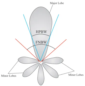
The radiation pattern represents directional variation of performance param-eters in a transmitter antenna. A trace of electric or magnetic field at a constant distance from the antenna is the amplitude field pattern whereas a similar trace of electric or magnetic power density is the amplitude power pattern. The ra-diation pattern is usually has bulging portions called lobes. Rara-diation lobes are high intensity directions surrounded by weaker radiation directions. The major lobe includes the direction of maximum radiation which is the desired radiation direction. Any lobe other than the major lobe is a minor lobe. The radiation pattern of an antenna changes depending on the distance from the antenna. This change in field pattern results that the space surrounding the antenna divided into three field regions: reactive near field, radiating near field (Fresnel) and far field (Fraunhofer). The reactive near field region starts from the radiating sur-face of the antenna and terminates about a wavelength of the transceived wave. In this region the energy decays very rapidly with distance from the radiating surface (energy decays with the third and fourth power of the distance) and the field pattern is nearly homogeneous although there are localized energy fluctua-tions. The radiating near field region is between reactive near field and far field
FNBW HPBW
Major Lobe
Minor Lobes Minor Lobes
Figure 2.1: A typical radiation pattern of an antenna.
regions. In this radiation field region the field pattern depends on the distance from the antenna and it begins to form lobes. If the antenna dimensions are very small compared to wavelength, the radiating near field region diminishes. The boundary between radiating near field and far field regions is defined as the distance 2D2/λ where D is the largest dimension of the antenna. Beyond this
distance is the far field region where the field pattern is well formed and does not vary with distance from the antenna. Here the energy decays with the square of distance from the radiating surface.
The radiation power density W of an antenna is the time average Poynting vector whereas the radiation intensity U is the directional power radiated from the antenna per unit solid angle. Radiation intensity U is a far field parameter and obtained by multiplying the radiation power density by distance square, U = r2W .
The beamwidth of an antenna is is a quantity associated with the radiation pattern. The angular distance between two identical points on opposite sides of the field pattern is defined to be the beamwidth. As a convention, half power
beamwidth (HPBW) is defined to be the angle between two sides of the field pattern where the radiation intensity is half of its peak value in the direction of maximum antenna radiation. Furthermore, first null beamwidth (FNBW) is the angle between first nulls of the field pattern. Figure 2.1 demonstrates radiation pattern, lobe and beamwidth concepts.
The directivity D of an antenna is the ratio of the radiation intensity U in a particular direction to the radiation intensity averaged over all directions U0 = Prad/4π. If a particular direction is not specified, it is taken to be the the
direction of maximum radiation.
D = U
U0
= U
Prad/4π
(2.1)
The gain G of an antenna is the ratio of the radiation intensity U in a partic-ular direction to the antenna input power intensity averaged over all directions. Again, if a particular direction is not specified, it is taken to be the the direction of maximum radiation. A constant called radiation efficiency ecd is defined in
order to relate input and radiated power intensities Prad = ecdPin. Radiation
efficiency embodies conduction and dielectric losses of the antenna. It does not include the mismatch loss between source and guiding device couple and the antenna. Thus directivity and gain can be related.
G = U
Pin/4π
= ecdD (2.2)
The bandwidth of an antenna is the range of frequencies where the antenna performance parameters individually have an acceptable value compared to those at the antenna center frequency.
The polarization of an antenna is the electromagnetic polarization of the radiated wave in a particular direction. If a particular direction is not specified,
it is taken to be the the direction of maximum gain. Polarization is categorized as linear, circular and elliptical. If the electric or magnetic field vector of the radiated wave at a point is always directed along a line at every instant of time, the field is said to be linearly polarized.
The input impedance ZA of an antenna is the impedance presented by the
antenna at its terminals, ZA = RA+ jXA. Here RA is the input resistance and
embodies power dissipations due to radiative and ohmic losses. XA is the input
reactance and represents reactive power losses.
As a consequence of reciprocity theorem, radiation pattern, radiation power density, radiation intensity, beamwidth, directivity, gain, bandwidth, polariza-tion and input impedance of an antenna are identical during transmission and reception.
Common radio antenna, half wavelength linear dipole (l = λ/2) is a standing wave antenna because the dynamic current distribution on the antenna has a standing wave pattern. For l = λ/2 the input reactance XA of the antenna
vanishes and the antenna is said to be resonant in analogy with a resonant RLC circuit [16]. At resonance the input impedance of the antenna is purely resistive and reactive losses due to XA are neglected.
2.2
Electromagnetics of Metals
Maxwell’s equations are sufficient to describe the interaction of metals with elec-tromagnetic fields [17]. Even if the metal is nanometer sized, quantum mechanics is not required. This is a result of the high density of free electrons in metals. High density of free electrons ensures very close electron energy levels and even nanometer sized metals can be explored classically.
Metals reflect electromagnetic waves for frequencies up to about visible. In this frequency regime metals are highly conductive and only negligible electro-magnetic wave penetrates into the metal. At higher frequencies dielectricity of metal becomes noticeable and wave penetration increases. This dispersive character of metals is described with the complex dielectric function ε(ω) since all electromagnetic phenomena depends on ε(ω). Furthermore, the underlying physics behind this dispersive character is the phase difference between electro-magnetic wave and free electron oscillation which arises due to the particular electron relaxation time τ of the metal.
Plasma model is a valid approximation over a wide frequency range for ex-plaining dispersive characteristics of metals [17]. In this model free electron gas of number density n is assumed to be moving against fixed background of posi-tive ion cores. The electron motion is a damped oscillation due to collisions with collision frequency γ which is due to the particular relaxation time of the metal, γ = 1/τ . τ is in the order of 10−14
s at room temperature, corresponding to γ = 100 THz. A simple representation of metallic band structure is also incorpo-rated into the effective electron mass m. Thus plasma model equation of motion for an electron subjected to an external time harmonic electric field E is
m¨x + mγ ˙x = −qE(t), (2.3)
where x is the electron displacement and q is the electron charge. For E(t) = E0e−iωt driving field, a particular solution to the equation of motion
for an electron is
x(t) = q
The complex amplitude of x(t) absorbs the phase difference between driving field and electron displacement. Thus the macroscopic polarization P = −nqx becomes
P = − nq
2
m(ω2+ iγω)E. (2.5)
Embedding polarization P to the electric flux, D = ǫ0ǫE = ǫ0E + P yields
D = ǫ0 µ 1 − ωp 2 ω2+ iγω ¶ E, (2.6) where ωp2 = nq 2
ǫ0m is the plasma frequency of the particular metal. Hence the complex dielectric function of a metal ǫ(ω) = ǫ1(ω) + jǫ2(ω) is obtained where
ǫ1(ω) = 1 − ωp2τ2 1 + ω2τ2, (2.7) ǫ2(ω) = ωp2τ ω(1 + ω2τ2). (2.8)
The plasma frequency ωp/2π and the corresponding plasma wavelength λp
of common metals are 3570 THz / 85 nm for Al, 1914 THz / 156 nm for Cu, 2175 THz / 138 nm for Ag and 2175 THz / 138 nm for Au [18]. The collision frequency γ of common metals are 175 THz for Al [19], 14 THz for Ag [20] and 6 THz for Au [21].
At frequencies ω < ωp and ω ≪ τ−1, metals are so conductive that only
negligible electromagnetic wave penetrates. Here ǫ2 ≫ ǫ1 and ǫ1 is negative.
Thus, the real and the imaginary parts of the complex refractive index ˜n =√ǫ = n(ω) + jκ(ω) becomes comparable in magnitude with
n ≈ κ =r ǫ22 = r
τ ωp2
2ω . (2.9)
The absorption coefficient α in Beer’s law describes how the intensity of the electromagnetic wave propagating into a medium attenuates. Since α = 2κωc , the absorption coefficient for ω ≪ τ−1
becomes
α = p2τωp
2ω
c (2.10)
The intensity of the electromagnetic wave penetrating into the metal decays with e−z/δ
, where δ = 2/α is defined as the skin depth of the particular metal. At frequencies ω < ωp and ω ≫ τ−1, ǫ(ω) is practically real, ǫ2(ω) ≈ 0, and
ǫ(ω) = 1 −ωp
2
ω2 . (2.11)
However, in this frequency band interband transitions cause metals behave differently. At higher frequencies ω > ωp, the dielectricity of metal becomes so
high that this is described by an extra dielectric constant, ǫ∞ (1 ≤ ǫ∞ ≤ 10)
ǫ(ω) = ǫ∞−
ωp2
ω2+ iγω (2.12)
Figure 2.2 shows real ǫ1(ω/2π) and imaginary ǫ2(ω/2π) parts of the complex
dielectric function of gold. The material data is taken from Palik’s Handbook of Optical Constants and used by Lumerical FDTD for numerical calculations.
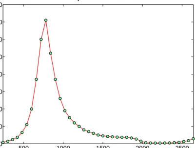
0 500 1000 1500 2000 2500 0.991 0.992 0.993 0.994 0.995 0.996 0.997 0.998 0.999 1 1.001 frequecny (THz) Re(eps) 0 500 1000 1500 2000 2500 0 0.002 0.004 0.006 0.008 0.01 0.012 0.014 frequecny (THz) Im(eps)
Figure 2.2: Real ǫ1(ω/2π) and imaginary ǫ2(ω/2π) parts of the dielectric function
of gold.
2.3
Resonant Optical Nanoantennas and
Appli-cations
Concentrating light in the nanometer scale, using subwavelength sized metallic structures, has recently developed into a new branch of photonics called plas-monics, or more descriptively nanophotonics which eponymously announces the overcoming of the diffraction limit. Plasmonics is a resonant phenomenon that is based on the interaction of light with conduction electrons in nanostructured metals [17]. It has the promise of merging photonic capacities with that of re-duced size integrated electronics. [22].
Nanoantennas enable optimum conversion of propagating light into subwave-length localized optical fields [1, 2, 4, 23–27]. Concentrating light leads to electric field enhancement [28]. Thus optical antennas allow manipulating light matter interaction in the reactive near field of the nanoantennas rendering them in-dispensable in many technological applications such as fluorescence microscopy, absorption spectroscopy, control of single molecule emission, extreme ultraviolet light generation, infrared photodetection, solar energy conversion and photother-mal tumor therapy [5–8, 12–14]. Hence nanoantennas are expected to find many applications in greatly improving the efficiency of the optoelectronic devices [23].
B1
B2
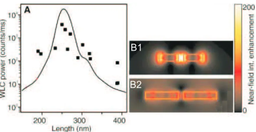
Figure 2.3: (A) Variation of WLSC power with antenna length, filled squares. Solid curve represents calculated near field intensity response without a y-axis. (B1 to B2) Calculated spatial near field on 10 nm above the dipole nanoantennas at λ = 830 nm. (B1) At resonance (B2) Out of resonance [1].
Incident light induces oscillations of the metal’s free electrons. Thus upon il-lumination several harmonic current waves with different amplitudes and phases are created within the antenna skin depth. At resonance interference of those current waves results in a standing wave. In other words, at resonance a collec-tive charge oscillation is created on the antenna which produces the enhanced reactive near field. The enhancement of the field is determined by the resonance properties. Unlike radio antennas, the reactive near field of nanoantennas are of importance because incident light is said to be confined in the reactive near field of the nanoantenna. Since current electronics is speed limited, the result-ing current wave on the nanoantenna cannot be manipulated by an electronic circuitry.
The pioneering work of M¨uhlschlegel et al in 2005 introduces the solid frame of optical antenna research [1]. They show that resonance depends on the antenna length and the polarization of the incident light. This is proved with numerical calculations and experimental demonstration. Gold dipole antennas fabricated on glass substrate are illuminated with picosecond linearly polarized laser pulses at λ = 830 nm. The enhanced near field of the resonant nanoantennas are used to boost nonlinear phenomena. The antennas lying along the polarization direction
Figure 2.4: Measured WLSC spectra of a resonant dipole nanoantenna for three different average power levels of the pulsed Ti:sapphire laser, excitation wave-length λ = 830 nm [1].
and of particular length generate white light supercontinuum (WLSC) radiation. WLSC generation is due to the third order optical nonlinearity of glass substrate and the optical power coming from the laser and sufficiently enhanced by the nanoantenna. Figure 2.3A shows WLSC power and near field enhancement for different dipole lengths. Figure 2.4 shows WLSC spectra coming from a resonant dipole, only short wavelength wing of the spectra is considered though.
Ghenuche et al illustrate the modes and the modal field distributions of res-onant nanoantennas [2]. In analogy with the standing current wave modes of the linear dipole radio antenna (l = nλ/2, n being an integer) [10], the modes of the nanoantenna are associated with the resonances using the relation between the antenna length L and the effective wavelength λef f : L = (n + 1/2)λef f
(n being an integer). As shown in figure 2.5 additional weaker field modulations along the sides of the nanoantennas address higher order resonant modes, namely 3λef f /2 and 5λef f /2 resonances. The 3λef f /2 resonance of the 500 nm long
stripe antenna occurs at λ = 710 nm (n=1 with λef f = 333 nm). However, the
same mode of the dipole consisting of 500 nm long stripes with 40 nm gap shifts to λ = 730 nm. That 5λef f /2 mode of the 1 µm long stripe appears at λ = 760
Figure 2.5: (a) Calculated spatial near field | E | and (b) | E |4 of the three types
of antennas at their respective resonance wavelength. (c) is obtained by convo-luting the | E |4 maps with a 200 nm waist 2D Gaussian profile and integrating
over the third dimension. [2].
Figure 2.6: (a) Luminescence map of the dipole nanoantenna for different wave-lengths. (b) Calculated convoluted | E |4 distribution over a dipole
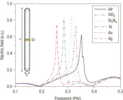
Figure 2.7: Far-field scattered electric-field amplitude calculated on the side of the dipole nanoantenna. The scattering resonance shifts with different materials filling the gap. εSiO2 = 2.36ε0, εSi3N4 = 4.01ε0, εSi= 13.35ε0 [3].
bandwidth of the optical antennas. Gold dipole nanoantenna fabricated on glass substrate is illuminated with femtosecond laser pulses to promote nonlinear ef-fects. The wavelength is scanned from 710 to 770 nm in steps of 10 nm. Since the measured luminescence is the signature of the resonant field enhancement, bandwidth of the dipole has been determined. The results are compared with numerical calculations as shown in Figure 2.6.
In addition to antenna length, nanoantenna resonance can be tuned by a mechanism similar to impedance matching [3]. Alu and Engheta, by means of numerical modelling, show that the response of dipole nanoantennas can be tailored dramatically by changing the material inside the dipole gap. Filling a few nanometer cube volume of the gap with materials of higher permittivities causes the optical dipole resonance to shift towards higher wavelengths. Figure 2.7 represents the tuning phenomena for a silver nanoantenna, h = 110 nm, r = 5 nm, g = 3 nm. However, the near field response is not given instead it is converted to far field. More complex tuning is achieved by filling the gap with parallel or series combinations of different permittivities as shown in figure 2.8.
Figure 2.8: Far-field scattered electric-field amplitude calculated on the side of the dipole nanoantenna. The scattering resonance shifts with different materials filling the gap. In the series combination of silicon and SiO2 the thicknesses
of the nanodisks are tSi = tSiO2 = 1.5 nm; in the series combination of SiO2 and gold,tSiO2 = 1.83 nm and tAu = 1.17 nm; in the parallel combination of silicon and SiO2, rin = 4.61 nm; in the parallel combination of silicon and gold,
Figure 2.9: (a) The cross resonant optical antenna structure. Gold nanoantennas on glass substrate have a cross section of 20nm × 20nm and a tip to tip distance of 10 nm. (b) The reference frame used. [4].
a)
b)Figure 2.10: Calculated spatial near field (a) In a plane at midheight of the structure, z = 10 nm (b) 5 nm above the upper antenna surface, z = 25 nm [4]. Optical antennas should lie along the polarization direction of the propagat-ing electromagnetic wave in order to resonate. However, a symmetrical geometric design can be used to eliminate this limitation [4]. Numerical calculations demon-strate that a structure consisting of two perpendicular dipole nanoantennas with a common feed gap is capable of resonating with any arbitrary polarization state carried of a propagating electromagnetic wave. Figure 2.9 shows this symmet-rical structure. The cross resonant nanoantenna is illuminated with a circularly polarized light at λ = 800 nm, figure 2.10 shows the obtained near field proving that the cross resonant nanoantenna can be used as a local and enhanced source of circularly polarized photons.
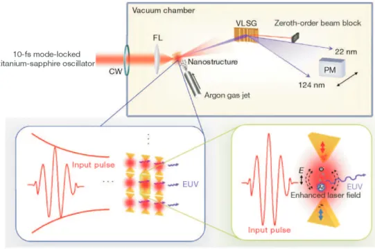
Figure 2.11: System for EUV generation. Ar, argon atom; CW, chamber window; FL, focusing lens; VLSG, varied-line-spacing grating; PM, photon multiplier. The laser is at λ = 800 nm with 100 kW peak power and 1.3 nJ pulse energy, producing intensity of 1011 Wcm−2
when well focused. [5].
d
Figure 2.12: (a) The bow-tie antenna structure and the reference frame used. h = 175 nm, d = 20 nm, t = 50 nm, θ = 30◦
(b) to (c) Calculated spatial near field of the resonant optical bow-tie (d) SEM image of the nanostructure used. Antennas are arranged as an array of area 10µm × 10µm. Edge lines are seen blurred due to high magnification. [5].
Figure 2.13: Open sleeve dipole structure. (a) Top view, dipole antenna is ori-ented in the y direction and two line electrodes (sleeves) are oriori-ented in the x direction. (b) Cross section through line 1. (c) Cross section through line 2. [6]. The local field enhancement of resonant nanoantennas has the potential to reduce the required high optical intensities of some applications. One such ap-plication is the high harmonic generation by focusing a femtosecond laser onto a gas and producing coherent extreme ultraviolet (EUV) light. However, the pro-cess requires high pulse intensities, greater than 1013 Wcm−2
, which is normally achieved via complex optical amplification techniques. Kim et al exploit the near field enhancement of bow-tie nanoantennas to obtain EUV light [5]. Their system is shown in figure 2.11. Gold bow-tie nanoantenna array fabricated on sapphire substrate is illuminated with femtosecond laser pulses of intensity 1011
Wcm−2
while facing the argon gas jet. As seen in figure 2.12, resonant bow-tie increases incident intensity by two orders of magnitude; hence, the threshold required to generate high harmonics is easily obtained. As a result, constructive interference of the emitted high harmonics from the individual antenna elements forms EUV radiation in the 22-124 nm wavelength range.
A photodetector with smaller active region is faster and has low capacitance. This results in high frequency operation with high output voltage. However, minimizing the photodetector size causes lower responsivity due to the diffrac-tion limit. Miller and colleagues overcome this challenge with the open-sleeve dipole antenna [6]. As seen in figure 2.13, a dipole gold nanoantenna is used to concentrate incident near infrared light into germanium active material. The
Figure 2.14: Calculated spatial near field on 25 nm above the SiO2 substrate
surface, (a) to (d) y polarized illumination. (a) Dipole with an air gap, resonant at λ = 904 nm. (b) Dipole with the gap filled with germanium, resonant at λ = 1271 nm. (c) Open sleeve dipole, resonant at λ = 1345 nm. (d) Open sleeve. (e) Open sleeve dipole, x polarized illumination. [6].
sleeves are used to extract the photocurrent. The measured photocurrent for y polarized incident light is 20 times higher than that for x polarized light at a very low bias voltage at λ = 1310 nm wavelength. Calculated near field, shown in figure 2.14 predicts this polarization response and proves how the sleeves change antenna characteristics.
Nanoantennas resonating at infrared wavelengths have the potential to collect the infrared energy either coming from the sun or reradiated from the earth. How-ever, this is impossible for the time being due to the lack of terahertz rectification of the induced current on nanoantennas. Nevertheless, Kotter et al fabricate in-expensive, flexible and large area periodic array of square loop gold nanoanten-nas resonating at infrared wavelengths [7]. Figure 2.15 shows the nanoantenna collector sheet. Thus, with the improvement of proper terahertz rectification techniques nanoantennas can be used to extend the limits of conventional pho-tovoltaic technology.
a
b
Figure 2.15: (a) SEM image of the square loop antenna array. (b) Nanoantenna collector sheet. [7].
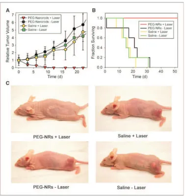
Nanoantennas are also used in biological sciences for example by utilizing them in photothermal tumor therapy [8]. Polyethylene glycol (PEG) coated gold nanorods (NR) resonating at λ = 810 nm are synthesized, shown in figure 2.16(A). PEG-NRs are stable in biological media and are passively accumulated in tumors through permeability. 72 hours after injection to mice, PEG-NRs disappear from blood circulation. After vascular disappearance of PEG-NRs, tumors of mice are irradiated with a laser of intensity 2 W/cm−2
at λ = 810 nm for 5 minutes. The calculated temperature for three different tumor depths of PEG-NR injected mice and the measured thermographic trace is shown in figure 2.16(B) and (C). Thus laser illumination causes PEG-NRs to heat up by means of the electric field enhancement discussed priorly and ablate the tu-mor tissue. Figure 2.17 presents the experiment results including the response of control groups. This promising work demonstrates tumor ablation by using nanoantennas as tumor specific catheters.
A
B
C
Figure 2.16: (A) TEM image of 13nm × 47nm synthesized gold nanorods. (B) Calculated temperature for three different tumor depths of PEG-NR injected mice. (C) Thermographic imaging of laser irradiated PEG-NR injected mice. [8].
Figure 2.17: Response of different treatment groups (A) Volumetric changes in tumor sizes after laser irradiation at λ = 810 nm, 2 W/cm−2
intensity, for 5 minutes. (B) Survival of treatment groups after laser irradiation (C) At 20 d after laser irradiation, PEG-NR injected mice is tumor free. [8].
A. Type Substrate A. Length Mode Wavelength Ref.
Dipole Glass 255 nm (20 nm gap) λef f /2 830 nm [1]
Stripe Glass 500 nm 3λef f /2 710 nm [2]
Dipole Glass 1040 nm (40 nm gap) 3λef f /2 730 nm [2]
Stripe Glass 1000 nm 5λef f /2 760 nm [2]
Dipole Glass 380 nm (60 nm gap) λef f /2 904 nm [6]
Table 2.1: Antenna type, substrate, antenna length, resonant mode and wave-length of the incident light in references tabulated.
Table 2.1 lists antenna type, substrate, antenna length, resonant mode and incident wavelength within the aforementioned references for comparison. Here we first infer the directly proportional relation between the incident wavelength and the required antenna length for λef f /2 resonant mode (first resonance).
This characteristics proves that freely accelerating electrons of the nanoantenna are driven by the incident harmonic electromagnetic field and resonate for a spe-cific antenna length. In accordance with the macro antenna theory, the relation between incident wavelength and resonant antenna length is explained with the dynamic current distribution on the antenna, and longer incident wavelengths require longer antennas. Secondly, we deduce that the resonance characteris-tics of a dipole nanoantenna is governed by individual nano stripes forming the dipole. Neglecting the small coupling effect between individual nano stripes, the dipole behavior is attributed to the stripe nanoantennas due to their individual current distributions in response to the driving field. The coupling due to the small gap increases the resonating wavelength of the individual stripe or in effect increases the effective wavelength (λef f ). Finally, we realize that λef f of higher
order resonant modes (i.e. 3λef f /2 and 5λef f /2 modes) are longer. We can
imagine higher order modes as series combinations of nanoantennas resonating at λef f /2 mode. However, that series combination has the maximum coupling
Chapter 3
NUMERICAL CALCULATIONS
In this chapter, nanoantenna and optical field interaction is investigated using industry standard commercial simulation software (Lumerical FDTD). Here we demonstrate the capability of nanoantennas in localized enhancement of light de-pending on their size, shape and surface properties. We first provide the near field response of various nanoantennas for λ = 1.5 µm linearly polarized incident op-tical radiation. Then, we describe the interaction of the opop-tical field (λ = 1.5 µm incident radiation), resonant stripe nanoantenna and As2Se3 (arsenic selenide)
substrate. Finally, we investigate the electromagnetic field interactions with a resonant stripe nanoantenna placed on a nonlinear (optical) As2Se3 substrate,
concentrating on the nonlinear optical interaction of the antenna near field with the substrate. Lumerical FDTD software allows implementation of the third or-der susceptibility term χ(3) and solves nonlinear FDTD. Since As
2Se3 is a highly
nonlinear material (χ(3) = 6.84 × 10⁻¹⁹
at λ = 1.5 µm), higher order effects such as the generation of new frequencies and harmonics, which require very large electric fields to become observable, can be induced with the electromagnetic enhancement achieved via resonant nanoantennas.
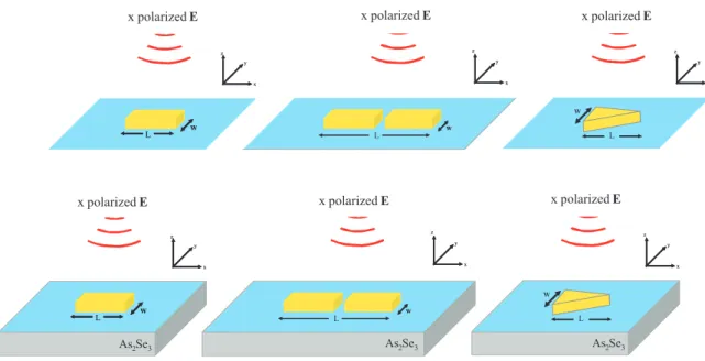
W W L x z y x z y x polarized E L L W W zz x polarized E L L W W As2Se3 As2Se3 x y x y W W L As2Se3
Figure 3.1: Setups and reference frame used in numerical calculations, L is the antenna length, w is the antenna width.
3.1
Optical Nanoantennas at
λ = 1.5 µm
In this section, we investigate stripe, dipole and single bow-tie gold nanoantennas for various antenna lengths. Steady state time averaged near field response of these three antenna types is calculated at the bottom face of the antennas for two different cases: when the antenna is in vacuum and when the antenna is on As2Se3 (arsenic selenide, n = 2.78 at λ = 1.5 µm). Calculated spatial
near field intensity is normalized with respect to the incident optical field. The incident light is a transverse electric field linearly polarized in the x direction at a wavelength of λ = 1.5 µm with 100 nm bandwidth. Figure 3.1 demonstrates setups and reference frame used in simulations. The blue surface represents the near field monitor at λ = 1.5 µm. L refers to antenna length and w refers to antenna width. All the calculations are made for fixed antenna width of w = 50 nm, except for the bow-tie nanoantenna where w = 100 nm is employed. Antenna thickness is always taken as 50 nm. Furthermore, 2 nm mesh size is used in all directions. In order to prevent reflections from the simulation boundaries,
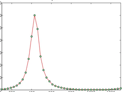
200 400 600 800 1000 1200 0 1000 2000 3000 4000 5000 6000 7000 Stripe Length (nm) E 2 Stripe in vacuum
Figure 3.2: Electric field peak intensity calculated for various lengths of the stripe nanoantenna in vacuum.
perfectly matched layers are utilized. Proper convergence is assured for each of the calculations.
The length of the stripe nanoantenna is scanned from 100 nm to 1300 nm with steps of 30 nm. Simulated dipole nanoantenna is comprised of two identical stripes with a constant 40 nm gap; therefore the dipole length is scanned from 240 nm to 2640 nm with 60 nm steps for comparison with the stripe antenna characteristics. Finally, the bow-tie response is calculated for the antenna lengths beginning from 100 nm up to 700 nm again with 30 nm steps.
Here we first provide the calculation results of the nanoantennas in vacuum. Figure 3.2 shows that the stripe nanoantenna in vacuum provides near field enhancement for a band of antenna lengths ceiling at about L = 430 nm which is shorter than λ/2. Therefore, an effective wavelength where L = λef f/2 = 430 nm
can be defined. Another near field intensity enhancement peak for L = λef f is not
observed as predicted by Ghenuche et al [2]. Spatial near field distribution for L = 430nm shown in figure 3.3 suggests that the field enhancement is a resonant
Figure 3.3: Electric field intensity distribution of the stripe nanoantenna in vac-uum for antenna length of L = 430 nm. First resonant mode is presented for two different intensity scales.
500 1000 1500 2000 2500 0 1000 2000 3000 4000 5000 6000 7000 8000 Dipole Length (nm) E 2 Dipole in vacuum
Figure 3.4: Electric field peak intensity calculated for various lengths of the dipole nanoantenna in vacuum.
one. At resonance, up to three orders of magnitude intensity enhancement and strong field confinement is observed.
Calculated dipole nanoantenna consists of two identical stripes with a 40 nm constant gap. Here L refers to the total length of two identical stripes and gap. Figure 3.4 indicates that the dipole nanoantenna in vacuum holds near field enhancement for a band of antenna lengths ceiling at about L = 820 nm. This implies that the dipole response is governed by the characteristics of individual stripes forming the dipole nanoantenna which is a result arrived at table 2.1 as well. However, resonant antenna length of the individual stripes is slightly lowered due to the coupling between them. Furthermore, spatial near field distribution for L = 820nm shown in figure 3.5 suggests that the dipole design contributes to higher near field intensities than of a single stripe inside the gap.
Figure 3.5: Electric field intensity distribution of the dipole nanoantenna in vacuum for antenna length of L = 820 nm. First resonant mode is presented for two different intensity scales.
1000 200 300 400 500 600 700 0.5 1 1.5 2 2.5 3 3.5 4x 10 4 Bow−tie Length (nm) E 2 Bow−tie in vacuum
Figure 3.6: Electric field peak intensity calculated for various lengths of the bow-tie nanoantenna in vacuum.
Simulated bow-tie nanoantenna is a single isosceles triangle with height L and base length w = 100 nm. Figure 3.6 indicates that the bow-tie nanoantenna in vacuum presents near field enhancement for a band of antenna lengths ceil-ing at about L = 430 nm, which is the same resonant length for nano stripe in vacuum. This implies that the resonance is related to the length of the antenna along the polarization direction of the incident light. As in the case of its radio equivalent, bow-tie nanoantenna is said to be middle bandwidth meaning that the range of frequencies producing resonance like behavior is wider than a lower bandwidth antenna [10]. This can be explained with the following analogy: the bow-tie nanoantenna behaves like a parallel combination of stripe nanoantennas. As a result, figure 3.6 includes more number of antenna lengths producing reso-nance like behavior and thereby near field intensity enhancement. Furthermore, the near field intensity enhancement of the bow-tie nanoantenna is an order of magnitude higher than the nano stripe. This is attributed to the sharp tip of the bow-tie. Figure 3.7 presents spatial near field distribution for L = 430 nm. Hence for an application where a single tiny optical spot of very high intensity is required, a resonant bow-tie design could be employed.
Figure 3.7: Electric field intensity distribution of the bow-tie nanoantenna in vacuum for antenna length of L = 430 nm. First resonant mode is presented for two different intensity scales.
200 400 600 800 1000 1200 0 500 1000 1500 2000 2500 3000 Stripe Length (nm) E 2 Stripe on As 2Se3
Figure 3.8: Electric field peak intensity calculated for various lengths of the stripe nanoantenna on As2Se3 substrate.
Regarding the case of nanoantennas on As2Se3 (arsenic selenide) substrate,
figure 3.8 reveals that the stripe nanoantenna on As2Se3 grasps near field
en-hancement for several bands of antenna lengths ceiling at about L = 190 nm, L = 670 nm and L = 1150 nm. The dielectricity of the As2Se3 substrate
(n = 2.78 at λ = 1.5 µm) opposes the dynamic charge distribution on the metal surface and introduces additional capacitance thereby lowering the reso-nant length of the nanoantenna. Hence we observe higher order resoreso-nant modes of the stripe which require longer antennas for the antenna lying in vacuum case. First resonance, so called the fundamental antenna mode, occurs at about L = 190 nm, where we can define an effective wavelength, L = λef f/2 = 190 nm.
Second resonance, 3λef f/2 mode, occurs at about L = 670 nm and third
reso-nance, 5λef f/2 mode, occurs at about L = 1150 nm, all similar to the definition
in the work of Ghenuche et al [2]. In accordance with table 2.1, λef f of higher
order resonant modes are longer. Furthermore, the dielectricity of the substrate also reduces the strength of resonance and thus decreases the intensity enhance-ment factor compared to the stripe lying in vacuum. Figures 3.9, 3.10 and 3.11
Figure 3.9: Electric field intensity distribution of the stripe nanoantenna on As2Se3 substrate for antenna length of L = 190 nm. First resonant mode is
Figure 3.10: Electric field intensity distribution of the stripe nanoantenna on As2Se3 substrate for antenna length of L = 670 nm. Second resonant mode is
Figure 3.11: Electric field intensity distribution of the stripe nanoantenna on As2Se3 substrate for antenna length of L = 1150 nm. Third resonant mode is
500 1000 1500 2000 2500 0 200 400 600 800 1000 1200 1400 1600 1800 2000 Dipole Length (nm) E 2 Dipole on As 2Se3
Figure 3.12: Electric field peak intensity calculated for various lengths of the dipole nanoantenna on As2Se3 substrate.
present spatial near field distributions for three different modes. The fundamen-tal resonant mode is more efficient than higher order modes but its shorter length requires more stringent fabrication methods. Spatial near field distributions sug-gest that higher order modes can be imagined as series combinations of antennas resonating at the fundamental mode.
Figure 3.12 indicates that the dipole nanoantenna on As2Se3 provides near
field enhancement for several bands of antenna lengths ceiling at about L = 360 nm,L = 1380 nm and L = 2340 nm. As in the case of dipole lying in vacuum, we calculated near field response of two identical stripes with a constant 40nm gap. The dipole response is again governed by the characteristics of the individual stripes on As2Se3. The resonant antenna length of the individual stripes is
slightly lowered due to coupling. Furthermore, higher refractive index substrate makes three different resonant modes observable albeit lowering the resonance strength. Dipole nanoantenna on As2Se3 characteristics is in accordance with
the results that we arrive at dipole in vacuum and stripe on As2Se3 cases. Figures
Figure 3.13: Electric field intensity distribution of the dipole nanoantenna on As2Se3 substrate for antenna length of L = 360 nm. First resonant mode is
Figure 3.14: Electric field intensity distribution of the dipole nanoantenna on As2Se3 substrate for antenna length of L = 1380 nm. Second resonant mode is
Figure 3.15: Electric field intensity distribution of the dipole nanoantenna on As2Se3 substrate for antenna length of L = 2340 nm. Third resonant mode is
1000 200 300 400 500 600 700 1000 2000 3000 4000 5000 6000 7000 8000 9000 10000 Bow−tie Length (nm) E 2 Bow−tie on As 2Se3
Figure 3.16: Electric field peak intensity calculated for various lengths of the bow-tie nanoantenna on As2Se3 substrate.
Figure 3.15 presenting the third resonant mode should also be noted due to several optical spots of high intensity with nanometer resolution.
Figure 3.16 shows that the single bow-tie nanoantenna on As2Se3 substrate
holds near field enhancement for several bands of antenna lengths ceiling at about L = 190 nm and L = 670 nm which are expectedly the same resonant antenna lengths for the nano stripe on As2Se3. This demonstrates that the resonance
depends on the antenna length along the polarization direction. However, the dielectricity of the substrate reduces the intensity enhancement factor compared to the bow-tie nanoantenna lying in vacuum. Figures 3.17 and 3.18 present spatial near field distributions for two different modes. The optical spots of high intensity in the second order mode are also identical to the second order mode of the nano stripe thereby implying the resonant antenna length as independent from the antenna shape.
Cubukcu et al investigates the response of stripe, dipole, single and double bow-tie nanoantennas on glass substrate for λ = 830 nm incident electric field linearly polarized along the antenna length [9]. The results in figures 3.19 and
Figure 3.17: Electric field intensity distribution of the bow-tie nanoantenna on As2Se3 substrate for antenna length of L = 190 nm. First resonant mode is
Figure 3.18: Electric field intensity distribution of the bow-tie nanoantenna on As2Se3 substrate for antenna length of L = 670 nm. Second resonant mode is
Figure 3.19: Electric field peak intensity calculated for various lengths of stripe and dipole nanoantennas on glass substrate are compared. For the dipole, an-tenna length is the length of the stripe forming the dipole and the gap is 20 nm [9].
3.20 are in agreement with our numerical calculations. However, the resonant lengths of the stripe (dipole) and single bow-tie (double bow-tie) nanoantennas do not coincide due to the curvature of the simulated structures. The ends of stripe along its length are rounded with a 20 nm radius of curvature, and the tip radius of curvature for bow-tie is taken to be 10 nm with an apex angle of 60◦
. As a result of the above numerical calculations we show that resonance char-acteristics of nanoantennas for a specific incident wavelength is governed by sub-strate, antenna length along the polarization direction of the incident electric field and the antenna shape. The refractive index of the substrate is inversely proportional with the resonant nanoantenna length and the near field intensity enhancement factor at resonance. This result is compatible with table 2.1, which tabulates simulation results for resonant nanoantennas on glass substrate. Fur-thermore, a specific incident wavelength causes resonant modes only for specific nanoantenna lengths. This result is also compatible with table 2.1 which man-ifests a directly proportional relation between the incident wavelength and the
Figure 3.20: Electric field peak intensity calculated for various lengths of single and double bow-tie nanoantennas on glass are compared. For the double bow-tie, antenna length is the length of the single bow-tie forming the double bow-tie and the gap is 20 nm [9].
resonant antenna length. Finally, the nanoantenna shape does not alter the res-onant antenna length fundamentally as long as the antenna length along the polarization of the incident field is preserved. However, the shape prominently affects near field intensity enhancement and antenna bandwidth.
0 10 20 30 40 50 60 70 80 90 100 101 102 103 104 z (nm) E 2 Resonant Stripe on As 2Se3
Figure 3.21: Electric field peak intensity calculated for several distances from the antenna dielectric interface for the fundamental resonance mode of the stripe nanoantenna on As2Se3 (arsenic selenide) substrate.
3.2
Resonant Stripe Nanoantenna on
As
2Se
3This section describes the interaction of the optical field, stripe nanoantenna at the fundamental resonance mode (λ = 1.5 µm, x polarized incident radiation) and As2Se3 substrate.
The interface between the resonating antenna and dielectric substrate is ex-posed to high electric field intensities albeit the penetration of that field into the dielectric is limited. As seen in figure 3.21, the near field enhancement of the resonating antenna vanishes about 90 nm away from the interface. This result is consistent with the rapid energy decay rate of the reactive near field region and demonstrates strong field confinement inside several cubic micrometers instead of propagation. Therefore, the resonating nanoantenna is a means for optimum conversion of propagating light into subwavelength localized optical field.
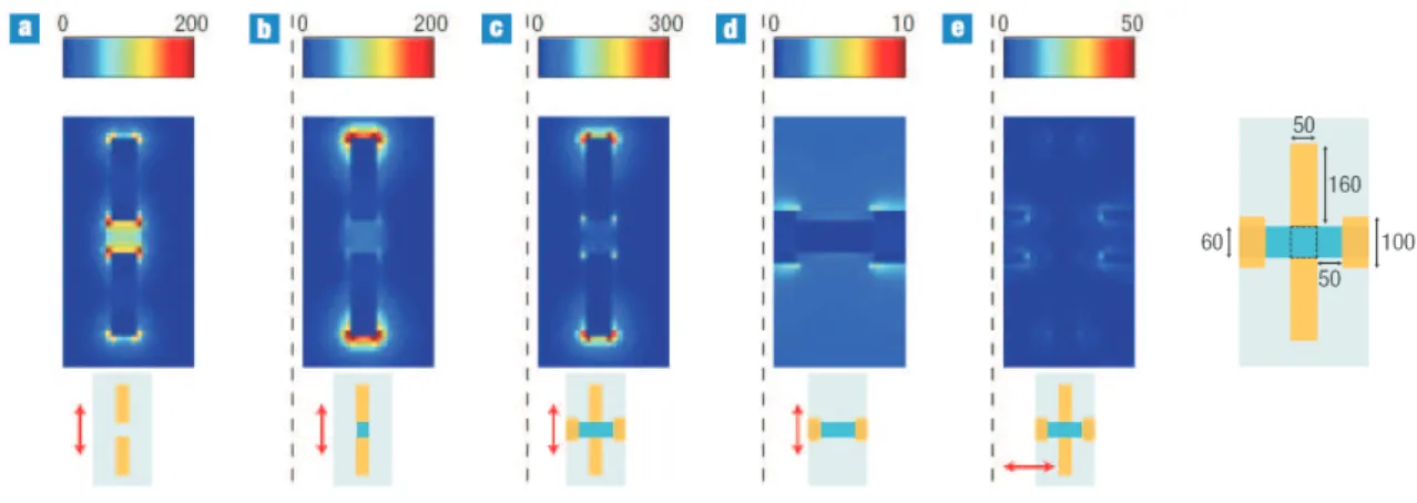
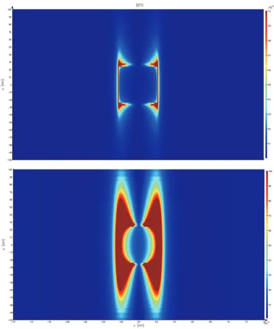
We also investigate components of the electric field intensity calculated at the antenna dielectric interface in order to understand nanoantenna radiation in gen-eral. Figure 3.22 shows field components of the resonating stripe nanoantenna. Interestingly, all three of Ex2, Ey2 and Ez2 have similar peak intensities albeit
their distributions are different. This phenomenon can be described by a simple model assuming electrons of the antenna as freely accelerating and driven by the incident harmonic electromagnetic field. This assumption vanishes the friction term γ in equation 2.3 (that is proportional to velocity) without fundamentally changing the resonance phenomena. Furthermore, in order to qualitatively dis-cuss the phenomena we should only consider first order effects due to the electric and magnetic field components of the incident field on the acceleration of the free charges. Here we ignore secondary interactions due to the charge radiation field and charges themselves. FDTD solutions take into account this secondary and higher order interactions due to the induced fields to obtain a converging solution.
As indicated in chapter 2, the electromagnetic radiation from a freely ac-celerating charge, for example in a plasma, known as the Larmor radiation, is directed perpendicular to the acceleration direction and shaped like a toroid cen-tered around the symmetry axis of the particle’s acceleration direction. There-fore, for x polarized incident electric field, the direction of resonant nanoantenna radiation should be around a toroid centered along the antenna axis. This leads to very large Ey and Ez components, and a small but finite contribution from
Ex. In figure 3.22 we already see prominent Ey2 and Ez2 components.
How-ever we should also be able to account for reasonably large Ex component. This
can be attributed to the y polarized magnetic field component of the incoming field. The magnetic force on the charges moving along the x axis is along the z direction because of the Lorentz force relation
F = −q ˙x × B(t). (3.1) Therefore, as x polarized incident electric field accelerates the charges along the x axis, y polarized magnetic field bents the charge motion towards the surface and bottom of the antenna harmonically, resulting acceleration along the z axis as well. An acceleration in the z direction is also accompanied with radiation field components Ex and Ey. However, magnetic forces are several orders of
magnitude smaller than electric forces. Therefore, exact computation of field components requires detailed numerical calculations.
It is interesting to note that the Ex2 and to an extent Ey2 components in
figure 3.22 have another very weak pairs of hot spots at the center of the nanoan-tenna in distinction to the Ez component suggesting that the source of this hot
spots are different. Furthermore, the higher order resonant modes mentioned in the previous section mainly have enhanced Ey and Ez type hot spots which is
suggesting that the resonance behavior of the nanoantenna is due to the main resonance along the antenna length.
The relative strengths of the field components depend on many factors affect-ing the resonance condition, i.e. antenna length and also width. Field strengths and computation eventually require simulation software. However, via our toy model, we show that we can account for the Ex2, Ey2 and Ez2 components by
taking into account the electron acceleration due to Ex and By components of
|E|^2
|E
x
|^2
|E
y
|^2
|E
z
|^2
Figure 3.22: Electric field intensity distribution in terms of field components for the fundamental resonance mode of the stripe nanoantenna on As2Se3.
3.3
Resonant Stripe Nanoantenna on
As
2Se
3and Nonlinear Effects
This section describes the interaction of high intensity optical field, stripe nanoantenna at the fundamental resonance mode (λ = 1.5 µm, x polarized incident radiation) and nonlinear (optical) As2Se3 (arsenic selenide) substrate.
Local optical field enhancement of resonant nanoantennas can be used for boosting nonlinear phenomena in the nano scale [1, 2, 5]. Since nonlinear effects require very large electric fields to become observable, the near field enhance-ment achieved around several cubic micrometers of resonant nanoantennas can be exploited for the generation of new frequencies and harmonics. As2Se3 is a
highly nonlinear (optical) material (χ(3) = 6.84 ×10⁻¹⁹
at λ = 1.5 µm) especially used in nonlinear fiber devices [29]. Here we investigate nonlinear optical inter-actions within the near field of a resonant stripe nanoantenna placed on As2Se3
substrate.
Lumerical FDTD allows implementation of the third order susceptibility term χ(3) and solves nonlinear FDTD. Here, the calculation is performed with
inci-dent transverse electric field (at λ = 1.5 µm) polarized along the antenna length. The incident field is a single pulse of peak amplitude 1e8 V/m with duration in the order of femtoseconds. The electric field intensity at the antenna dielectric interface is monitored during the pulse transition, and then transformed into the frequency domain by fast fourier transformation. As a result, position and wave-length dependent electric field intensity plots of the antenna dielectric interface are obtained.
Figures 3.23, 3.24, 3.25 and 3.26 present electric field intensity spectrum along a line, in the x direction, grazing the top left corner of the antenna. Therefore, all of the plots are given for the same y = 25 nm position. The 190 nm long and
−160 −140 −120 −100 −80 −60 −40 −20 0 500 1000 1500 2000 −4 −3 −2 −1 0 1 2 x position (nm) 150fs pulse length wavelength (nm) log( Ex 2)
Figure 3.23: Ex2 spectrum calculated at different x positions. The source has
150 fs pulse length at 1.5 µm. Ex2 is normalized with respect to the source peak
intensity.
50 nm wide resonant nanoantenna lies between x = −95 nm and x = 95 nm x and y = −25 nm and y = 25 nm y positions of the simulation area. Since near field response of the nanoantenna is symmetrical in the xy plane with respect to the antenna center, electric field intensity spectrum at different x points along the top edge of the antenna up to x = 0 is sufficient to analyze the phenomenon. The wavelength spectrum is restricted in the 400 nm to 2000 nm range, and normalized with respect to the peak intensity of the incident field. The calcula-tions are made for two different pulse lengths of 150 fs and 300 fs. Furthermore, Ex2and Ey2 spectrum are given separately for each of the different incident pulse
lengths. Since the third order optical nonlinearity of As2Se3is isotropic, sufficient
field intensity provided by the source and enhanced by the resonant nanoantenna produces nonlinear effects in terms of both Ex and Ey field components.