Analysis of an arbitrary conic section profile and thin dielectric cylindrical reflector illuminated by an E-polarized complex source point beam

(1)

2012 International Conference on

Mathematical Methods in Electromagnetic Theory

ANALYSIS OF AN ARBITRARY CONIC SECTION PROFILE AND THIN

DIELECTRIC CYLINDRICAL REFLECTOR ILLUMINATED BY AN

E-POLARIZED COMPLEX SOURCE POINT BEAM

Taner Oğuzer1_{, Fadıl Kuyucuoğlu}2_{, Ibrahim Avgin}2_{, Ayhan Altıntaş}3

1_{Electrical and Electronics Eng. Dept., Dokuz Eylul University, Buca, 35160 Izmir, Turkey} 2_{Electrical and Electronics Eng. Dept., Ege University, Bornova, 35100 Izmir, Turkey}

3_{Dept. Electrical and Electronics Eng., Bilkent University, 06800 Ankara, Turkey}

Abstract - We simulated arbitrary conic section profile and thin layer dielectric reflector using the Method

of Analytical Regularization (MAR) techniques. The reflector is assumed to be illuminated by a complex source point type feed antenna in E-polarization mode. We obtained excellent accuracy and convergence of our simulation.

I. INTRODUCTION

Reflector antennas have many applications such as in modern communication systems hence so many studies are done to reveal their useful properties. One can carry out simulations based on formulation of the electromagnetic boundary value problem (BVP). This kind of reflector can be thought of a transparent micro mirror device and can be used in the optical range systems. Thus similar electromagnetic BVP type solution can be applied to these micro mirror systems. In both applications the size of the reflector is greater than the wavelength.

The electromagnetic BVP based formulation of the larger size reflectors illuminated by a beam field is important, thus various accurate techniques have been developed in the literature. We studied a reflector where we regarded a two dimensional reflector’s surface E-polarization alone. In the full-wave modeling of the reflector systems, finite-difference time-domain method is of the oldest technique. For it requires huge number of unknowns due to the discretization of large physical domain and the far field radiation fulfillment. For the thin layers, the volume equivalence theorem based on the method of moments (MoM) formulation can be used alternatively where the basis functions are chosen as pulses on circular arcs. The convergence of the solution is not guaranteed in this implementation also. One can also expect that in the conventional MoM, non-realistic CPU times may occur. Generally it is known that the MoM can be applied to small and medium size reflectors (up to 10 wavelengths). Another approach is the high frequency techniques like GO, PO, PTD. They work much faster however they do not reproduce the results well.

Another serious alternative is the method of analytical regularization (MAR) [3]. In MAR, the kernel of the singular integral equations (SIE) is separated into two parts, the more singular part (usually static) and the remainder. Then choosing the global basis functions like in MoM, the more singular part is analytically inverted by using some special techniques. The remainder leads to the Fredholm second-kind matrix equation that provides a convergent numerical solution. By using the analytically producible Green’s function technique having a logarithmic singularity, the SIE-MAR is extended to the 2D-PEC reflectors of noncircular contours for both polarizations [4-5]. More exact full wave analysis of the reflector problems having imperfect material cases are performed by the SIE-MAR technique. In [6], assuming the noncircular contour the scattering problem is studied for the uniformly and non-uniformly resistive (i.e. edge-loaded) cases.

Here the resistive case simulation in [6] is extended. The resistive case works for very thin layers but if thickness increases more, then the electric field amplitude in the front side differs from back side of the thin layer. Then the electric resistivity (R) is not enough and the magnetic resistivity (S) should also be used with R. We apply the general thin layer boundary conditions (TLBC) presented in [2]. But the cross resistivity (W) is not considered and it is taken zero. So our thin dielectric reflector is assumed as the single layer but the lossy dielectric can be simulated. This is a better modeling than the resistive one until the thin layer boundary condition validity is violated. The SIEs obtained from TLBC are reduced to the coupled matrix equation system by using MAR techniques. The accuracy and convergence is checked by numerical results and the radiation patterns are compared with the MoM solution.

(2)

II. FORMULATION

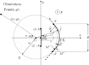
The problem geometry associated with a thin dielectric with the thickness h and arbitrary profile front fed reflector illuminated by a Complex Source Point (CSP) feed is presented in Figure 1. The 2-D cross section of the reflector is defined as conic-section profile and it may be an elliptic, parabolic or hyperbolic arc. Here we only note that they differ in the value of so-called eccentricity, e, so that e < 1 for an ellipse; e=1 for a parabola and e > 1 for a hyperbola.

Figure 1: Problem Geometry

The feed is located at the near geometrical focus of the reflector and a closed contour is defined as C that is the completed the reflector surface M by an aperture S. Additionally one thing has to be said that the M (metal) part of the reflector surface does not cross the CSP branch and also the circular arc S of the total contour C must be continuous curvature at the reflector edge points.

The rigorous formulation of the considered boundary value problem can be stated in terms of the Helmholtz equation, Sommerfeld radiation condition far from the reflector and source, the thin layer boundary conditions on M, and an edge condition such that the field energy is limited in any finite domain around the reflector edge. Collectively, these conditions guarantee the uniqueness of the problem solution [1].

The thin layer boundary conditions are a well-established model of a thin penetrable material sheet. It can be written as the following equations:

[E r_T( ) _E r_T( )] 2 ( ) ( ) _ R r n r   _J_z, J_z _[H r_T( ) _H r_T( )], r M_ ₍₁₎

[H r_T( ) _H r_T( )] 2 ( ) ( ) _ S r n r   _M_t, M_t _[E r_T( ) _E r_T( )], r M_ ₍₂₎

where subscript “T” indicates the tangential field, the superscripts “- “ and “+” relate to the front and back faces of reflector, respectively, and the unit normal vector

n



is directed to the inside that the feed is located. The unknown surface current densities Jz and Mt are called electric and magnetic type induced sheet currents.

For relatively thin layer (koh<<1), R and S parameters can be written as follows,

R( / 2)i  / cot[   / ( ₀ ₀)k h₀ / 2] S( / 2)i  / cot[   / ( ₀ ₀)k h₀ / 2] (3) These R and S parameters are defined for infinite flat sheets and also |r |1 assumption is considered (that is

the high contrast case). The R and S can also be used for the smoothly curved surface.

The incident electric field and the tangential magnetic field will be taken as the beam-like form generated by the CSP, given as (1) 0 ( ) 1 ( ) ( ) ( ) inc in in z z s T E r E r H k r r H r i n           ₍₄₎ where rs(x₀ibcos , y₀ibsin )

 _{. This incident field function has two branch points which should be}

connected with a branch cut. Its maximum is in the φ = β direction. Also parameters b and β are the aperture width and beam aiming angle respectively. Also (x yo_, o) indicates the real position coordinates.

With the aid of the auxiliary potential expressions and by using TLBC, the scattered fields can be obtained as,

(3)

( ') ( | ' |) ' ( ') ( | ' |) ' ( ) and 0 ( ) ' in Z o t o z z z M M j J r G k r r dl M r G k r r dl E R J r M J r S n           



  



     (5) ( ') ( | ' |) ' ( ') ( | ' |) ' ( ) and 0( ) ' in Z o t o T t t M M i J r G k r r dl M r G k r r dl H S M r M M r S n  n n  _ _  _ _ _ _ _ _   



  



     (6)

where the scalar Green’s function G is a Hankel function of the zeroth order and first kind satisfying the radiation condition; i.e. (1)

0

[ ( ), '( ')] ( / 4) ( o )

G r r   i H k R , R r( ) r'( ') . Assume that the curve M can be characterized with the aid of the parametric equations xx( ), yy( ) 0 | |  in terms of polar angle, φ. Besides define the differential lengths in the tangential direction at any point on M as  l a  ( ) ,  l' a  ( ') ' respectively. Also  ( )r( ) / [ cos ( )] a   , ( )  is the angle between the normal on M and the x-direction, ( )  is the angle between the normal and the radial direction. Then we extend the surface-current densities Jzand Mtwith zero

value to S. Then the above sets of equations are modified on the complete contour C made of S and M.

To continue on the MAR based formulation all parameters should be written in terms of the Fourier series (FS) representations. Firstly the incident fields are expressed in terms of the FS coefficients. Furthermore for the working procedure of the formulation that is to make computations more economic, we add and subtract the similar functions from the originally given ones. These are the functions at the full circle of the closed contour C and introduced as follows.





(1) (1) 0 0 ( , ') ( o ) [2 o sin | ' | /2 ] A  H k R H k a   (7) (1) (1) 0 1 ( ) ( , ') ( ') sin[| ' | /2] [2 sin(| ' | /2)] ' o o o H k R B a k a H k a n            (8) (1) 2 (1) 0 0 ( , ') cos[ ( ) ( ')] ( ) ( ') [ | ( )_o '( ') |] ( ) [2 _o sin(| ' | /2)] S           H k r  r    H k a   (9) (1) (1) 0 1 ( ) ( , ') o ( ) sin[| ' | /2] [2 sin(| ' | /2)] o o H k R R a k a H k a n            (10) The functions A and S have also continuous first derivatives and their second derivatives with respect to φ and φ’ have only logarithmic singularity and hence belong to

L

₂. Therefore their FS coefficients decay as

1.5 1.5

(| | | | )

O n   m   on the curve C. The other two functions B and R have no singularity at all even in each term. So it is expected to decay faster than the functions A and S. Their corresponding FS coefficients can be computed by FFT algorithm effectively. So this provides us to solve reasonably larger geometries.

After some known functions extracted from the original kernels of the SIEs, then the more singular parts are tried to be inverted. Firstly the SIE in equation (5) is semi inverted by Fourier inversion procedure. The other one in equation (6) is converted to a dual series form and it is inverted by RHP technique. Finally we end up with the two coupled algebraic equation system and they constitute a matrix system as follows.

   1 2 1 2 1 2 1 2 3 4 5 m _mn n m m mn mn mn mn n m m mn mn mn mn mn nm mn n m y _Z y P x A A B B x T m D D C C C C C m E            _ _    _ _ _ _ _       _{} _{}_    (11)

where xm and mm are the coefficients for Jz and Mt surface current density functions respectively. In the above matrix equation, the elements of the main matrix are not given here in detail. Then together with the large index assumptions for cylindrical functions, this enables one to prove that 2

, | mn|

m n Z



  



. By the similar treatment one can find that _| _|2

m

m P



  



provided that the branch cut associated with the CSP aperture does not cross the reflector contour M. In this case the infinite matrix equation (11) is of the Fredholm second kind. Hence the Fredholm theorems guarantee the existence of the unique exact solution and also the convergence of approximate numerical solution when truncating (11) with progressively larger sizesN_tr.

III. NUMERICAL RESULTS AND CONCLUSION

Formulation presented above is justified by simulating computer codes to obtain unknown current density functions, radiation patterns and directivities. The same problem is also solved by MoM and the pulse type basis functions are chosen in the volume equivalence theorem based formulation. Figure 2(a) presents the forward directivity obtained from MAR versus Ntr for two different eccentricity factors. As expected, while the truncation

(4)

number increasing, the directivity converges for both factors. In Figure 2(b), the relative accuracy in directivity defined as D=|D Ntr1 - D |/DNtr Ntr is given in logarithmic scale. Figure 2(c) demonstrates the relative error in surface current densities in MAR for e=1 (parabola case). These errors are so-called maximum norm and defined as Ntr 1 Ntr Ntr

n n n

J=max|x_  -x |/max x _{for electric current density and} Ntr 1 Ntr Ntr

n n n

=max|m -m |/max

M  m

 for

magnetic current density. The functions J and M are plotted in logarithmic scale versus truncation number. These errors also present a decaying nature and so the convergence property of the presented formulation is tried to be verified. Figure 3 shows the normalized radiation patterns of both MAR and MoM cases for two different thicknesses. It is seen that the accuracy of the MAR is decreasing when the thickness is increasing. Since the validity of the thin layer boundary conditions is decreasing but the MoM simulation does not depend on this boundary condition.

Figure 2. (a) Directivity versus Ntr (b) The relative Figure 3. The normalized radiation patterns (a)

error in directivity (c) The relative errors in the surface for h=0.1λe, R/Z=0.017+0.34i,S*Z=-0.34+6.89i

The other parameters are f=10λ, d=15λ, kb=3, h=0.1λe, (b) for h=0.2λe, R/Z=0.0076+0.15i,S*Z=-0.15+3.08i

εr=20+2i. The other parameters f=24λ,d=20λ,kb=3,e=0(circle) εr=20+2i. A circle approximating parabola.

A 2-D penetrable sheet with the arbitrary conic section profile illuminated by an E-polarized CSP has been analyzed using a semi-inversion approach for the E-polarization case. Simulation results have been compared with MoM and good agreement has been observed.

REFERENCES

[1.] D. Colton, R. Kress, Integral Equation Method in Scattering Theory (Wiley, 1983).

[2.] E. Bleszynski, M. Bleszynski, T. Jaroszewicz, “Surface-integral equations for electromagnetic scattering from impenetrable and penetrable sheets,” IEEE Antennas Propagat. Mag., vol. 35, pp. 14-25, 1993.

[3.] A.I. Nosich, “Method of analytical regularization in the wave-scattering and eigenvalue problems: foundations and review of solutions,” IEEE Antennas Propagat. Mag., 42, 34-49, 1999.

[4.] T. Oguzer, A. I. Nosich, A. Altintas, “E-polarized beam scattering by an open cylindrical PEC strip having an arbitrary conical-section profile,” Microwave Optical Tech. Letters, vol. 31, pp 480-484, 2001

[5.] T. Oguzer, A. I. Nosich, A. Altintas, “Analysis of an arbitrary conic section profile clylindrical reflector antenna, H-polarization case,” IEEE Trans. Antennas Propagat, vol. 52, pp 3156-3162, 2004.

[6.] T. Oğuzer, A. Altintas, A I. Nosich, “Integral equation analysis of an arbitrary-profile and varying-resistivity cylindrical reflector illuminated by an E-polarized CSP beam,” J. Opt. Soc. Am A, vol. 26, pp. 1525-1532, 2009.