An animation system for rigid and deformable models

('tllnpuf. & (iraphin Vol. 17. No. I, pp. 71-77, 1993 Printed in Great Bntam.

0097-8493/93 $6.00 + .00 © I 99 3 Pergamon Press Ltd. Technical Section

AN ANIMATION SYSTEM FOR RIGID

AND DEFORMABLE MODELS

UCuR GOD0KBA Y and BOLENT OzGO<;::

Bilkent University, Department of Computer Engineering and Information Science, 06533 Bilkent, Ankara, Turkey

and YILMAZ TOKAD

Bilkent University, Department of Mathematics, 06533 Bilkent, Ankara, Turkey

Abstract-We describe a system for the animation of rigid and deformable models. The system uses the approaches from elasticity theory for animating the models. Two different formulations, namely the primal

and the hybrid formulations, are implemented so that the user could select the suitable one for an animation

depending on the rigidity of the models. Collision of the models with impenetrable obstacles and constraining model points to fixed positions in space are implemented for use in the animations.

I. INTRODUCTION

This paper discusses an animation system that is im­ plemented for the animation of rigid and nonrigid ( de­ formable) models. The system is built on top of a modeling system for representing 3D free-form objects, that uses Superquadrics [ l] and Bezier surfaces [ 2] as modeling techniques, and regular deformations [ 3] and Free-Form Deformations[ 4] for deforming these models to obtain irregular, free-form objects [ 5]. The static models obtained by these methods can be ani­ mated using the techniques discussed in this paper. The system is implemented using C language [ 6] on a Unix* workstation environment ( it runs on Sun_3 and Spare workstations). The implementation uses the

facilities provided by Sun Viewt _{system such as win­}

dows, panels, and menus [ 7].

The use of computer graphics and numerical meth­ ods for 3D design and modeling provides an interactive environment in which designers can formulate and represent shapes of objects. Modeling the shapes as a composition of geometrically and algebraically defined primitives, simulating scenes with shading and texture, and producing usable design images are the most im­ portant requirements for application areas such as Computer-Aided Design and Computer-Aided Man­ ufacturing.

Currently, most of the methods used for modeling are kinematic. This becomes a major drawback when

we want to create realistic animation because these methods are passive; they do not interact with each other or with external forces. To achieve realism in animation a model should be able to follow predefined paths while still moving in an interesting manner and interacting with other models as real physical objects would do.

To build and animate active models, physically­ based techniques should be used. These techniques

fa-* Unix is a trademark of AT&T Laboratories.

t Sun View is a registered trademark of Sun Microsystems.

71

cilitate the creation of models capable of automatically synthesizing complex shapes and realistic motions that

are attainable only by skilled animators. Physically­

based modeling achieves this by adding physical prop­

erties to the models. Such properties may be forces, torques, velocities, accelerations, kinetic and potential

energies, heat, etc. Physical simulation is then used to

produce animation based on these properties. To this

end, solution of the initial value problems is required

so that the course of a simulation is determined by objects' initial positions and velocities, by the forces

and torques applied to the object along the way, etc.

Another aspect in realistic animation is modeling

the behavior of deformable objects. To simulate the

behavior of deformable objects, we should approximate a continuous model by using discretization methods, such as finite difference, and finite element method. For finite difference discretization, a deformable object could be approximated by using a grid of control points where the points are allowed to move in relation to one another. The manner in which the points are al­ lowed to move determines the properties of the de­ formable object. Simulating the physical properties ( such as tension and rigidity) static shapes exhibited by a wide range of deformable objects ( including string, rubber, cloth, paper, and flexible metals) can be mod­ eled. For example, to obtain the effect of an elastic surface, the grid points are connected by springs. The physical quantities cited earlier should be used to sim­ ulate dynamics of these objects. Various

researchers[8-I 3] presented discrete models that are based on elas­

ticity and plasticity theory and use energy fields to de­

fine and enforce constraints for animating deformable objects.

The plan of this paper is to first present a short de­ scription of the methods proposed by Terzopoulos et al.[ 11, 12, 14] for elastically deformable models, and inelastic models. We will then explain the implemen­ tation details of these methods in the context of our system, and algorithmic solution of the problems, such

as collision of flexible models with impenetrable ob­ stacles, etc. Then, some simulation results representing the features of the system are given.

2. NONRIGID MODELS

To animate nonrigid objects in a simulated physical environment, we should use the methods of elasticity theory. Elasticity theory provides methods to construct the differential equations that model the behavior of nonrigid curves, surfaces, and solids as a function of time. Real materials exhibit both elastic and inelastic behavior. Some materials undergo perfectly elastic de­ formations so that when the forces acting on the ma­ terials are removed, objects restore themselves to their natural shapes completely. However, there are other materials, such as cloth, paper, etc. which restore themselves to their initial shapes slowly ( or partially) upon removal of the forces that cause deformations.

To model elastic materials, physical properties such as tension and rigidity should be simulated. In this way, static shapes of a wide range of deformable objects, including string, rubber, cloth, paper, and flexible metals, can be modeled. Dynamics of these materials can be simulated by including physical properties, such as mass and damping. The simulation involves nu­ merical solution of the partial differential equations that govern the evolving shape of the deformable object and its motion through space [ 12].

Viscous and plastic processes within the models evolve a reference component, which describes the natural shape, according to yield and creep relation­ ships that depend on applied force and/or instanta­ neous deformation. Simple fracture mechanics results from internal processes that introduce local disconti­ nuities as a function of the instantaneous deformations measured through the model [ 15 ] .

2.1. Deformable models

Deformable models can be formulated by using the intrinsic or material coordinates of points in a body !J. For a solid body u = ( U1, u_2, u_3), for a surface u =

( u 1 , u2) and for a curve u = ( u i) denotes the material

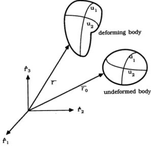
coordinates. The Euclidean 3-space positions of points in the body are given by time-varying vector-valued function r(u, 1) = [r₁ (u, 1), r₂(u, 1), r₃(u, t)]. The

body in its natural rest state is given by r0(u) =

[r?(u), rg(u), rg(u)] (Fig. I). The equations of mo­ tion for a deformable model can be written in La­ grange's form as

a

(

) ar be(r)

-_{at at} µ - + "' -+ -- = f(r t)

I at /jf ' ' (I)

where µ(u) is the mass density of the body at u, -y(u)

is the damping density of the body at u, f (r, t) is the net externally applied force, and e(r) is the energy functional that measures the net instantaneous poten­ tial energy of the elastic deformation of the body. The shape of a body is determined by the Euclidean dis­ tances between nearby points. As the body deforms, these distances change. Let u and u + du denote the

Fig. I. Geometric representation of a deformable body for primal formulation. Reprinted with permission from "Elast­ ically Deformable Models" by D. Terzopoulos, J. Platt, A.

Barr, and K. Fleischer. ACM Computer Graphics, 21 (Proc.

SIGGRAPH 1987) 205-214. Copyright 1987, Association for Computing Machinery, Inc.

material coordinates of two nearby points in the body. The distance between these points in the deformed body in Euclidean 3-space is given by:

di= L Guduiduj, i,j

where the symmetric matrix: ar ar

Gu(r(u)) = -·­_{aui au}

j

(2)

(3)

is the metric tensor, which is a measure of deformations ( the dot indicates the scalar product of two vectors).

Two 30 solids have the same shape ( differ only by a rigid body motion) if their 3 X 3 metric tensors are identical forms ofu = [u_1, u_2, u_3]. Two surfaces have

the same shape if their metric tensors Gas well as their

curvature tensors Bare identical forms ofu = [ u1, u2].

The components of the curvature tensor are: a2_r

Bu(r(u)) = n·--, _auiau

j (4)

where n = [n1, n2, n3] is the unit surface normal. Two

space curves have the same shape if their arc length

s(r(u)), curvature K(r(u)), and torsion r(r(u)) are

identical forms of u = [ ui]. See [ 16] for a detailed dis·

cussion of these formulations.

Using the above differential quantities, potential energies of deformation for use in Lagrangian equations can be defined as the norm of the difference between the fundamental forms of the deformed body and those of the undeformed body. This norm measures the amount of deformation away from the natural shape so that the potential energy is zero when the body is in its natural shape and increases as the model gets increasingly deformed away from its natural shape.

An animation system for rigid and deformable models 73

shape are denoted by the superscript 0, then the strain energy for a curve can be defined as

c(r) =

L

+

+

where w 1, w2_{, and w}3 _{are the coefficients for the curve,}

showing the amount of resistance to stretching, bend­ ing, and twisting, respectively. The strain energy for a surface can be defined in a similar way:

c(r) =

L

IIG - G

IIB -

wt( u1, u2). Analogously, a strain energy for a deform­

able solid is

c(r) =

L

IIG -

where the weighted matrix norm 11 • llw• involves the

weighting functions w b( U1, u2, U3).

These energies denote the amount of energy to re­ store the deformed objects to their natural shapes. The net external force in Lagrange's equations is the sum of various types of external forces, such as gravitational force, spring forces, viscous forces, etc.

The weighting functions in the above energies ( w j( u 1 , u2) and wt( u 1 , u2) for an elastic surface) de­

termine the properties of the simulated deformable material. The weighting function wb(u1, u2) deter­

mines surface tensions and sheer strengths that mini­ mize the deviations of the surface's actual metric coef­ ficients Gu from its natural coefficients Gi. As wb is

increased, the material becomes more resistant to length deformation, with w l I and wh determining this

resistance along U1 and u2 , and wb = w11 determining

the resistance to shear deformation. The functions wt( u1, u2) control surface rigidities that act to mini­

mize the deviation of the surface's actual curvature coefficients Bu from its natural coefficients

si.

wt is increased, the material becomes more resistant

to bending deformation, with wf I and w�2 determining

this resistance along U1 and u2, and wb = w11 deter­

mining the resistance to twist deformation. To simulate a stretchy rubber sheet, for example, we make wb rel­ atively small and set wt = 0. To simulate relatively stretch resistant cloth, we increase the value of wb. To simulate paper, we make wb relatively large and we introduce a modest value for wt. Springy metal can be simulated by increasing the value of wt. Since w &< u) and wt( u) are functions of material coordinates

u, we may vary the material properties over the surface,

and we may introduce local singularities such as frac­ tures and creases [ 11, 12] .

To create animation with deformable models, the differential equations of motion should be discretized by applying finite difference approximation methods and solving the system of linked ordinary differential equations of motion obtained in this way.

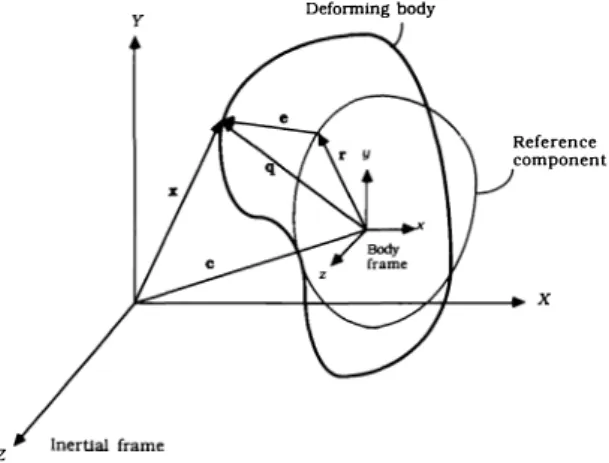
The above formulation for elastically deformable models is called primal formulation. Another for­ mulation, called hybrid formulation represents a de­ formable body as the sum of a reference component

r(u, t) and a deformation component e(u, t) (Fig. 2).

The positions of mass elements in the body relative to <f> is given by

q(u, t) = r(u, t)

+

In this formulation, deformations are measured with respect to the reference shape r. Elastic deformations are represented by an energy c(e), which depends on the position of a reference frame <f> whose origin co­ incides with the body's center of mass and it should be evolved over time according to the rigid body dy­ namics to have a rigid body motion besides its elastic motion.

The nonquadric energy functional in primal for­ mulation causes a nonlinear elastic force asssociated with the deformable body to appear in the partial dif­ ferential equations of motion. Nonlinearity results be­ cause the elastic force attempts to restore the shape of the deformed body to a rest shape. The advantage of nonlinear elasticity is that it is in principle the most accurate way to characterize the behavior of certain elastic phenomena. However, it can lead to serious practical difficulties in the numerical implementation of deformable models for animation. The hybrid for­ mulation offers a practical advantage for fairly rigid models, whereas primal formulation becomes un­ practical due to the nonquadric energy functional with increasing rigidity and complexity of the rest shapes[l 1, 14].

3. IMPLEMENTATION OF THE PRIMAL FORMULATION

Steps of animation of deformable models using pri­ mal formulation are as follows:

First, we should calculate the total external force for each point of the model that is discretized using body

Deforming body

z

Reference component

Fig. 2. Geometric representation of deformable models for hybrid formulation. Reprinted with permission from "Mod­ eling Inelastic Deformation: Viscoelasticity, Plasticity. Frac­ ture" by D. Terzopoulos and K. Fleischer, ACM Computer

Graphics, 22 (Proc. SIGGRAPH 1988) 269-287. Copyright 1988, Association for Computing Machinery, Inc.

coordinates of the model. In order to achieve this, we should add the forces effecting a point, which are grav­ itational, viscous, collision, and constraint forces. The constraint forces are taken into account in the following way: When a constrained point tends to move, an op­ posite force for bringing it back to its original position is calculated and added to the total external force for that point. Each constrained point has an effect on the total external force for all points in the model depend­ ing on the difference between the body coordinates of the points. This effect is calculated according to an exponential distribution function. This method for calculating constraint forces gives good results for small time steps. For larger time steps, the model points make small oscillations since this approach corresponds to a corrective action.

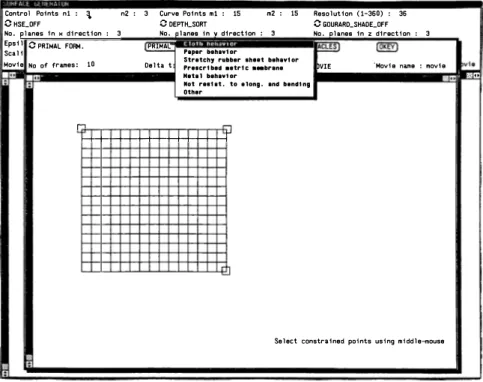
The constrained points are specified by the user in­ teractively. The system displays a grid specifying the body coordinates of each point existing in the model to be animated and the user selects the points to be constrained during the animation ( the points that will not move during the animation) using mouse buttons ( Fig. 3). In other words, any point on a model could be constrained to a fixed location in space so that when the model is animated, the constrained points remain in their initial positions. The constraint force that con­ nects a material point Uo on a deformable model to a point Po in space by a spring is

f,(u, t) = k(Po - x(uo, t))o(u - Uo), (9)

where k is the spring constant and o is the unit delta

function.

More complicated constraints are being studied for future versions of our implementation ( such as

point-Control Potnts n1 : \ 0HSE_OFF

n2 : 3 Curve Potnts mt : 15 C DEPTH_SORT

to-point constraints, for connecting two points on dif­ ferent models to simulate articulated figures, point-to­ line constraints, for controlling the motion of the

models, etc. ) . However, some implementation prob­

lems occur with the current formulation.

The forces due to the collision of deformable mo.dels with impenetrable obstacles are calculated using the obstacle's implicit (inside-outside) function. The ob­ stacle exerts a repulsive force on the deformable model that can be calculated as a function of the obstacle's implicit function such that the force grows quickly if the model attempts to penetrate the obstacle. This is

achieved by creating a potential function c _exp(Vf(x)/

E) around each obstacle, where f is the obstacle's im­

plicit function, V denotes the gradient, and c and E are

constants determining the properties of the obstacle. In our system, the user can select different obstacles to exist in an animation sequence by the help of a menu. Ellipsoids, toroids, hyperboloids are possible choices for an obstacle. The repulsive force due to an impenetrable obstacle is

fc(u, t) = -c((Vf(x)/E)exp(-f(x)/E)· n)n, (10) where n(u, t) is the unit surface normal vector of the deformable body's surface.

The second step, after calculating the total external force for each point on the discrete model and speci­ fying the value of the weighting functions, is the dis­ cretization of the partial differential equations using finite difference methods on the discrete mesh of nodes. For this purpose, we calculate the finite differences that are used to calculate the stiffness matrix K. Expressing the grid functions x[m, n] and E[m, n] as :!f and!. in grid vector notation, which are denoting the 3D

po-m2 : 15 Resolution (1-360) : 36 0 GOURARO_SHAOE_OFF No. planes in H d11"'ectton : 3

Epstl C PRIMAL FORM.

No, lanas tn v direction : 3 No. olanea tn z dtractton : 3

PRIMAL:

Scali Paper behavt or

Movie No of frames: 10 Delta t Stretchy rubber shHt bebav1 or Prescrt bed aetrt c ••brene Neta 1 llehav1 or

bVIE "Movie name : movie Not restat. to along. and bandtng

Other

r,

...

t-+-+-+--+-+-+--+-+-+-+-+-+-+-+-i

Select constrained points using middle-mouse

Fig. 3. Screen dump during the specification of the parameters for an animation.

An animation system for rigid and deformable models 75 sitions of model points and elastic force for each model

point stored in M X N vector for an M X N discrete grid of a deformable model, elastic force can be written in vector form as

�=Kt�)·.! , ( 11) where K is an MN X MN matrix. K is a sparse and banded matrix. This becomes a major advantage when we solve the simultaneous system of second-order or­ dinary differential equations. The band structure of the matrix K is shown in Fig. 4 .

The mass densityµ( u1, u2) and the damping density

-y( 11,, 112) are discretized as grid functions µ[m, n] and -y [m. n]. Let M be the mass matrix, an MN X MN diagonal matrix with the µ [ m, n] variables as diagonal elements, and C be the damping matrix constructed similarly from -y[m, n]. Then the Lagrange equations can be expressed in grid vector form by the simulta­ neous system of second-order ordinary differential equations

d2_{x dx}

M dt2

+

+

=

has been discretized into the grid vector f which rep­ resents the grid function f[m, n].

We integrate this system through time using a step­ by-step procedure. Evaluating K(_!) at time t

+

d2_x

d-_{ 2

=

dx

d-

=

t -

-into Eq. ( 12), we obtain the semi-implicit integration procedure

A,.!1+a1

=

Fig. 4. The band structure of the stiffness matrix K.

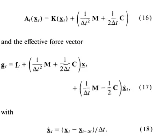
where the MN X MN matrix

A,(.!,)= K(.!,)

+

+

C)

and the effective force vector g,

=

+

+

(17) with

if, =(.!, -.!,-a,)/ t!.t. ( 18)

Applying the above semi-implicit procedure, we can evolve the dynamic solution from given initial con­ ditions �o and ifo at t = 0 . During each time step, we solve a sparse linear algebraic system [ Eq. ( 15)] for the instantaneous configuration .!J+a1 using the preced­

ing solution.!, and if, [ 12].

Implementation of the hybrid formulation follows the same steps described for the primal formulation. The only difference is the sparse, banded stiffness ma­ trix K is constant. The equations of motion can be expressed in semidiscrete form by a system of coupled ordinary differential equations. The system contains two ordinary differential equations for the translational and rotational motion of the model as if all of its mass is concentrated at its center of mass, and a system of ordinary differential equations whose size is propor­ tional with the size of the discrete model. These equa­ tions are solved in tandem for each time step with re­ spect to the initial conditions given[ 14].

4. SIMULATION EXAMPLES

We have implemented both primal and hybrid for­ mulation in our system so that the user can interactively select between them. In this way, the primal formu­ lation can be selected for highly nonrigid models, and the hybrid formulation can be selected for highly rigid models.

The linear system of equations obtained by a semi­ implicit time integration procedure as explained in the previous section can be solved by different linear system solvers. Since the stiffness matrix is sparse and has a special band structure, Conjugate Gradient method for solving linear systems as described in [ 17] can be used. This method uses the sparsity property to gain effi­ ciency in solving the equations. We have also used LU decomposition and back substitution to solve the equations.

In Fig. 5, we have used the primal formulation and the material properties are adjusted to simulate a membrane not resistant to elongation or contraction, and not resistant to bending (w1 _{= 0, w}2 _{= 0) . In this}

Fig. 5. A highly nonrigid surface constrained from 3 comer falls (initially, the surface is flat).

Fig. 6. A moderately rigid surface constrained from different points on its edges exerted a downward force (Initially, the

surface is flat) .

from three corners and falls by the effect of the grav­ itational force.

In Fig. 6, we have used the hybrid formulation and set the material properties to simulate a moderately rigid object ( such as a thin metal plate). The model is constrained from different points on its edges and a downward force is exerted on it.

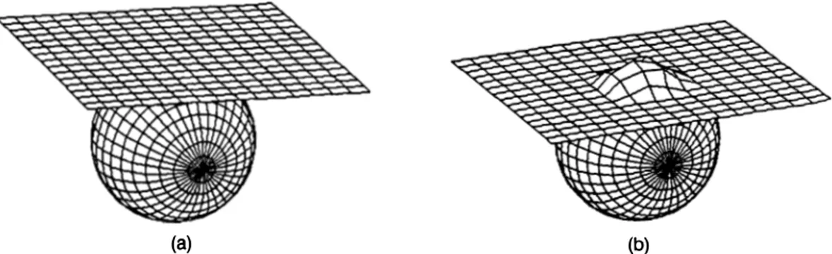
In Fig. 7, an elastic model not resistant to elongation or contraction and not resistant to bending falls on an impenetrable obstacle that is an ellipsoid. The deform­ able model takes the shape of the obstacle when it col­ lides with it as it is seen. To get better results in collision simulations, either we should take a very small time step or we should use an adaptive time stepping. Other­ wise, we may detect collisions very late, namely after the model points penetrate the obstacle too much.

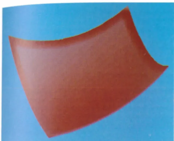
Shaded versions of these simulations are given in Figs. 8, 9, and IO.

(a)

5. CONCLUSION

In creating good computer animation, the focus is not on the problem of completing a given motion task, but more importantly on how this task is to be per­ formed by the animated character. All the elements involved in an animated character must cooper1;tte in synchronized harmony. Most of the animation systems generated up to now leave the burden of generating realistic animation to the animator. To remedy this problem, fundamental principles of traditional ani­ mation, such as squash and stretch, exaggeration.follow

through, and overlapping action[ 18] should be for­

malized as high level constructs.

Physically-based modeling has emerged as a means of creating realistic animation. It proposes methods to create active models that react to applied forces, to constraints, to ambient media, or to impenetrable ob­ stacles, as one would expect from real physical objects. In this way, computer animators are unconcerned with the kinematic details of animations, knowing that physics will dictate the low-level motions.

Physically-based modeling adds new levels of rep­ resentation to object description in addition to ge­ ometry. Forces, torques, velocities, kinetic and poten­ tial energies, heat, and other physical quantities are used to control the creation and evolution of models. To construct the differential equations of the motion of the models, different techniques, such as Lagrangian equations, constraint methods, the principle of virtual work, can be used. Constraint methods, which are highly suitable for this purpose, unify the creation of complex models with the control of the motion of the models. After constructing the equations of motion for the models, the equations should be solved using fast numerical methods.

In this paper, we explained a system for animating rigid and deformable models. The system uses both the primal formulation and the hybrid formulation for animating these models so that the user can decide which one to use in an animation considering the ad­ vantages and disadvantages of each formulation. Our aim as a future work is to modify the equations of motion proposed for deformable models[l2] in such a way that constraint forces will be taken into account as external forces. This approach allows modeling and animating articulated bodies consisting of rigid and nonrigid parts by creating complex models from

sim-(b)

An animation system for rigid and deformable models 77

Fig. 8. Shaded version of the simulation in Fig. 5. Fig. 9. Shaded version of the simulation in Fig. 6.

Fig. 10. Shaded version of the simulation in Fig. 7. pier primitives using point-to-point constraint. Also,

other constraints, such as point-to-path etc., can be

used to control the motion of the models. REFERENCES

I.A. H. Barr, Superquadrics and angle-preserving transfor­ mations. IEEE Comp. Graph. Appl. 1( I) 11-23 (January 1981).

2. P. Bezier, Numerical Control-Mathematics and Appli­

cations, John Wiley and Sons, London ( 1972).

3. A. H. Barr, Global _{and local deformations of solid prim­} itives. Comp. Graph. 18(3) 21-30 (July 1984). 4. T. W. Sederberg and S. R. Parry, Free-form deformation

of solid geometric models, ACM Computer Graphics

(Proc. SIGGRAPH), 20(4) 151-160 (August 1986). 5. U. Gildiikbay and B. Ozgiic, Free-form solid modeling

using deformations, _{Computers & Graphics,} 14(3)

491-500 ( 1990).

6. B. W. Kernighan and D. M. Ritchie, The C Programming

Language, Prentice Hall, Inc., Englewood Cliffs, NJ

(1978).

7. Sun _{Microsystems, Sun View Programmer's Guide,}

Mountain View, CA (1986).

8. J.E. _{Chadwick, D. R. Haumann, and R. E. Parent, Lay­} ered construction for deformable animated characters,

ACM Computer Graphics, 23(3) (Proc. SIGGRAPH 1989), 243-252 (July 1989).

9. J. Platt and A. Barr, Constraint methods for flexible

models, ACM Computer Graphics, 22( 4) (Proc. SIG­ GRAPH 1988) 279-288 (August 1988).

10. A. Pentland and J. Williams, Good vibrations: Modal dynamics for graphics and animation ACM Computer

Graphics, 23(3) (Proc. SIGGRAPH 1989) 215-222 (July

1989).

11. D. Terzopoulos and K. Fleischer, Modeling inelastic

deformation: Viscoelasticity, plasticity, fracture, ACM

Computer Graphics 22( 4) (Proc. SIGGRAPH 1988) 269-278 (August 1988).

12. D. Terzopoulos, J. Platt, A. Barr, and K. Fleischer, Elast­

ically deformable models, ACM Computer Graphics 21 ( 4)

(Proc. SIGGRAPH 1987) 205-214 (July 1987).

13. A. Witkin, K. Fleischer, and A. Barr, Energy constraints on parameterized models, ACM Computer Graphics

21(4) (Proc. SIGGRAPH 1987) 225-232 (July 1987).

14. D. Terzopoulos and A. Witkin, Physically based models

with rigid and deformable components, IEEE Comp.

Graph. Appl. 8(6) 41-51 (November 1988).

15. J. D. Faux and M. J. Pratt, Computational Geometry for

Design and Manufacture, Halstead Press, Horwood, NY (1981 ).

16. M. P. Do Carmo, Differential Geometry of Curves and

Surfaces, Prentice-Hall, Englewood Cliffs, NJ ( 1974 ). 17. W. H. Press, B. P. Flannery, S. A. Teukolsky, and W. T.

Vetterling, Numerical Recipes in C: The Art of Scientific

Computing, Cambridge University Press, Cambridge,

U.K. ( 1986).

18. J. Lasseter, Principles of traditional animation applied to 30 computer animation, ACM Computer Graphics 21 ( 4)