Efficiency of CONWIP production lines: a simulation study

n s » ύ іш еш ά '-· W ’ i * ' *** i ' ·, '♦ « · I ¿ 13М Й Ш 0» : Ш Ш ^ .' ■' ■ . •’"•s:^··; i·. w » (· <4hw m лщ / 1 Ж t s ^ \Q S Á f

EFFICIENCY OF CONWIP PRODUCTION LINES; A SIMULATION STUDY

A THESIS

SUBMITTED TO l'HE DEPARTMENT OF MANAGEMENT AND GRADUATE SCHOOL OF BUSINESS ADMINISTRATION

OF BILKENT UNIVERSITY

IN PARTIAL FULFILLMENT OF THE REQUIREMENTS FOR THE DEGREE OF

MASTER OF BUSINESS ADMINISTRATION

By

A. ERCÜMENT BÖLÜKBA§ June, 1994

T s

' ß 6 f

I certify that 1 have read this thesis and that in iny opinion it is fully adequate, in scope and in quality, as a thesis for the degree of Master of Business Administration.

Assist. Prof. Erdal EREL

I certify that I have read this thesis and that in my opinion it is fully adequate, in scope and in quality, as a thesis for the degree of Master of Business Administration.

Assist. Prof. Murat MERCAN

I certify that I have read this thesis and that in my opinion it is fully adequate, in scope and in quality, as a thesis for the degree of Master of Business Administration.

Assist. Prof. Neiat KARABAKAL

Approved by Dean of the Graduate School of Business Administration

ABSTRACT

EFFICIENCY OF CONWIP PRODUCTION LINES: A SIMULATION STUDY

A. Ercüment Bölükbaş M.B.A.

Supervisor : Assist. Prof. Erdal Erel June, 1994, 53 pages

Today in industiy production lines are stochastic systems. These systems are designed to optimize some performanee measures; the perfoimance measures are generally the throughput and WIP of the systems. Managers want to maximize throughput and minimize WIP. To achieve these goals, several designs are tested. Aim of this study is to develop some guidelines for the design of CONWIP type of systems.

ÖZET

CONWIP ÜRETİM SİSTEMLERİNİN VERİMİ: BİR SİMULASYON ÇALIŞMASI

A. Ercüment Bölükbaş MBA Yüksek Lisans Tezi

Tez Yöneticisi: Yrd. Doç. Dr. Erdal Erel Hazia'an, 1994, 53 sayfa

Günümüzde üretim hatları belirsizlikler içeren sistemlerdir. Bu sistemler performansları en iyi olacak şekilde dizayn edilmelidirler. Performans ölçüleri genelde sistemin verim hızı ve üretim zaman stoğu miktarıdır. Yöneticiler sistemin verim hızını en yüksek, üretim zaman stoğunıı en düşük seviyede tutmak isterler. Bu hedeflere ulaşmak için birçok değişik dizaynlar yapılır. Bu çalışmanın amacı CONWIP türü sistemlerde planlamacılara bazı öneriler getiiTnektir.

ACKNOWLEDGMENT

I would like to thank to Assist. Prof. Erdal Erel for his invaluable supervision tliroughout this thesis. I would also like to thank to Assist. Prof Murat Mcrean and Assist. Prof Nejat Karabakal for their help. Finally, I would like to thank to Department of Management of Bilkent University for providing me an MBA education.

TABLE OF CONTENTS

1. INTRODUCTION ...I

2. THE FUNCTION OF WIP IN SERIAL PRODUCTION LINES... 6

3. LITERATURE REVIEW... 8

3.1 The Role of Work-In-Process Inventoiy In Serial Production Lines... 8

3.2 Describing the Processing Time of Stations... 10

3.3 Buffer Space Allocation in Assembly Lines ... 12

3.4 Push and Pull Production Systems ... 13

3.5 CON WIP : A Pull Alternative to Kanban ... 15

4. METHODOLOGY ... 17

4.1 Introduction ... 17

4.2 Notation... 21

4.3 Assumptions ... 21

5. EXPERIMENTATION...23

5.1 Determination of the Number of Stations ...23

5.2 Analysis of Equally Distributed Containers ...25

5.3 Analysis of Demand Variation...27

5.4 Analysis of Full Demand and Low Demand...29

5.5 Effect of C and M ...31

5.6 Effect of Transportation T im e...34

6.1 Contribution of This Study... 39

6.2 Results... 40

6.3 Further Research Areas... ,...41

APPENDIX... 42

REFERENCES ... 52

The analysis and design of produetion lines have been studied in the research literature for the last 25 years. Several aspects of production lines have been analyzed. However, the problem of WIP inventory transfer is still an area for further research.

A production line consists of serial woi'kstations. Parts pass through these workstations in the same sequence. Having been processed in a workstation, parts are placed into containers (buffers) between workstations and they are picked up by the downstream workstation. There exists production lines with and without containers (buffers). There are two major types of buffer design in production lines.

Fixed Buffers: Inventory within the system waits in containers between workstations within a small distance from the operators. The upstream operator places a part into the container when the work on the part is finished. Tlie downstream operator takes the part out of the container when he gets idle. For the upstream operator to use the container, there must be at least one available place in the container for the part to be placed. For the downstream operator to take a part from the container, there must be at least one part waiting in the container. This buffer design is used when workstations are close to each other.

1. INTRODUCTION

Moving Buffers: This type of buffer design is used when workstations are separated from each other. The containers (buffers) are filled by the upstream operator. The full containers are then sent to the next workstation. The movement of a container from one workstation to another takes time which is called the transportation time. Wlten a fiill container arrives to a workstation, the operator of that workstation takes the parts out of that container one by

one completing the required task. When the container gets empty, it is free to camy new parts.

The buffer design used in any production line affects the utilization of capacity in that line. The utilization of capacity in a production line is rarely 100%. Because the workstations can be blocked or starved.

This study deals with the design of moving buffers. The containers are filled by upstream workstations and they are sent to the downstream workstations.. When all the parts in the container are taken out by the downstream workstation, the container is free to carry new parts. The output rate of the system (throughput) varies depending on the number of containers in the production line.

The production lines in the industi'y generally work either in push or pull mode. Push and pull refer to the means for releasing jobs into a production facility. In a push system, a job is started on a start date that is computed by subtracting established lead time from the date the material is required, either for shipping or for assembly. A pull system is characterized by the practice of downstream work centers pulling stock from previous operations, as needed.

The production line to be analyzed here is CONWIP. There are several studies on push and pull production systems. CONWIP production lines are pull-based production systems which share the advantages of both pull and push production systems. In fact, CONWIP production lines are hybrid production lines using the rules of both pull and push production lines.

CONWIP, is tlie abbreviation of COnstant Work In Process, wliich contains tlie characteristics of both pull and push systems. A basic CONWIP line is in Figure 1.

Backlog Cards Raw Materials \ __________ Parts

□ o n o

□ - 0 - n - Goods Inv.Finished

o

The operation of a CONWIP production line is controlled by the signals sent from finished goods inventory. A backlog card accompanies each part in the production syslcjn. The number of cards used in the system set the WIP level for the production line. When a customer arrives, if there is an empty card, a signal is sent to the beginning of the line. This signal authorizes the start of a new job. Under CONWIP, a job will not be started unless a signal code is received and there is a place in the system for that job. The backlog queue is for keeping track of sequence of production with the help of backlog cards (in Figure 1). When a signal arrives, a job is released to the system in the order of backlog cards. After the signal have been received, jobs are pushed between workstations in series. The signals are received by the backlog queue which allows explicit control over which parts are to be produced and in which sequence (Speannan, Woodruff and Hopp, 1990).

The CONWIP production lines set the WIP level in the system and measure the throughput, which is the output per unit time. The advantage of CONWIP is that it is applicable to a wider variety of production environments compared to the situations applicable with either push or pull systems.

In a CONWIP system, the backlog cards carrying signals, traverse a circuit that includes the entire production line. A card is attached to a standard part at the beginning of the line.

When the part leaves the last station, the card is removed and sent back to the beginning backlog queue where it waits to be attached to another part. Under no circumstances are expediters allowed to force the start of work without a signal, even if the first workstation in the production line gets idle (Spearman, Woodruff and Hopp, 1990).

CONWIP is similar to a technique used in air traffic control. On days with heavy air traffic, a departing plane will sometimes be held on the ground at the originating airport rather than be allowed to take off and remain in a holding pattern at the congested destination airport. Because the object is to avoid delays at the destination airport (in the air), planes are held even if take-off runways are free at the originating airport. The result is greater safety and lower fuel consumption with no added delay. (Spearman, Woodruff and Hopp, 1990).

Under CONWIP, sufficient number of jobs must be placed in the production line so that bottleneck workstation is seldom idle, but not so much that jobs wait a great deal of time. Then the line will reach maximum tlu'oughput without excessive flow time or WIP. In a CONWIP line, WIP will tend to collect at the bottleneck. The basic production systems may be summarized in Figure 2 which compares push, pull and CONWIP systems (Spearman, Woodruff and Hopp, 1990).

Pure Push Lower Level Inv Lower Level Inv Lower Level Inv

\

o > 0

-o —

The objectives of this thesis are to design a CONWIP production line and to perform some experiments via simulation to improve the efficiency of the production line by analyzing the throughput and WIP. A simulation model is developed and by varying the decision variables such as the number of stations, the number of containers and capacity of the containers, the effect of them on the production line will be analyzed.

This thesis is organized as follows; section 1 is introduction. The function of WIP in serial production lines is analyzed in Section 2. Section 3 is devoted to literature review including what has been done in the past 25 years. The methodology is given in Section 4, including the assumptions and the decision variables. The experimentation starts with Section 5.

2. THE FUNCTION OF WIP IN SERIAL PRODUCTION LINES

WIP is the inventoiy carried in a production system. Generally it does not include raw material inventory and finished goods inventory. Inventory carried in a production system, in our case are held in containers (buffers). The main reason of placing containers between workstations is to provide each workstation some degree of independent action. Containers also reduce the effect of machine breakdown, since they keep parts as safety stocks. (Conway, et al., 1988).

Without intervening WIP, the workstations in series will interfere with each other and production capacity will be lost unless two workstations in series finish each production cycle at precisely same instant. Even if they have the same average variable processing times, the first station sometimes finishes a cycle before the second. The first station must wait to dispose of its finished piece before it begins the next piece and it is said to be

blocked. Similarly, if the second workstation finishes a cycle before the first and must wait

for input material until the first finishes, the second station is said to be starved. Both blockage and starvation mean that a process is prevented from starting, and hence, potential production capacity is lost. Provision for buffers between such stations increases capacity by reducing the frequency and severity of blockage and starvation (Conway, et al., 1988).

A similar but more serious loss occurs if a machine is unexpectedly shut down for any reason: a breakdown, broken or missing tooling, operator unavailability etc. Some amount of WIP between the stations provides a grace period during which operation continues when another station is shut down ( Conway, et al., 1988). Buffers also allow two workstations to work on different products, even if there is a significant setup time required to change from one product to another. Effective use of WIP is further complicated because the position of buffers are as important as their capacity. There· are some locations where

buffers increase cost without any commensurate benefit, and others where even a single buffer is highly productive. (Conway, et ah, 1988).

But the role of WIP is to deal with short term transients; it is not capable of overcoming long term imbalance in capacity. Even so, the capacity of a facility varies importantly as a function of the amount and location of buffers. The zero WIP production capacity is related to the probability that all workstations ai'e simultaneously in operation. At the other extreme; the infinite WIP capacity is the long term average capacity of limiting stage; this is the bottleneck in the design. The classical investment cost of WIP, is probably the least important price one must pay for WIP. However, it is often dominated by the facilities cost of the equipment required to support and move WIP, and the cost of space it occupies. These considerations include substantial elements of opportunity cost that make them harder to quantify than capital costs.

Perhaps the most important cost of WIP is the effect on manufacturing lead-time or flo w

time. Flow time is the ti?ne required to move a piece tlirough manufacturing process, from

entry on the factory floor to completion of the last production stage. The sum of processing times for the piece is the minimum possible value of flow time, and everything above that is associated with WIP, including material handling. If for example, material handling was instantaneous and there was one unit of WIP in buffers between each pair of workstations, each piece would spend roughly as much time waiting as being processed, and the ratio of How time to total processing time would be approximately 2 to 1. It is therefore, suiprising to learn that a ratio of 10 to 1 is hard to achieve even in a modem plant and that ratios in excess of 100 to 1 are common; a piece that could be produced in a single day requires one or more months to pass through the plant. The consequences of this phenomenon is critical. ( Conway et al., 1988).

The design of production lines have been studied for a long time. Analytical methods and simulation were used several times in the studies for the design of production lines. Besides the studies on the design of production lines, work-in-process inventory transfer in these production lines is a critical concept in literature. WIP is a major cost factor for any manufacturing company. The studies are generally on reducing the amount of WIP in a production system which will reduce the costs. WIP transfer in production lines are analyzed under the categories of push, pull and CONWIP production systems. These analysis are summarized below.

3.1 THE ROLE OF WIP INVENTORY IN SERIAL PRODUCTION LINES

The role of Work-in-Process inventory in serial production lines have been analyzed by simulation (Conway, Maxwell, Mc.Clain and Thomas, 1988). They argue that, in serial production systems, storage may be required in the system to avoid interference due to lack of syncluonization.

They have analyzed the distribution and quantity of WIP inventory that accumulates in the system. They have defined WIP as inventoiy after the first step in manufacturing and before the last which did not include raw materials and finished goods inventory. The puipose of WIP has been defined as; "To give each stage o f a production system some degree o f

independent action."

3. LITERATURE REVIEW

The objectives of their study were to determine where WIP is most effective and to measure the benefit of WIP as a function of quantity.

They emphasized that potential production capacity is lost due to blockage or starvation. The requirement for WIP between workstations increases production capacity by reducing the frequency and the severity of blockage and starvation.

They have made an experimental study with the following considerations: 1) Identical workstations

2) Non-identical workstations 3) Unreliable workstations

'fheir method of analysis used computer models to simulate production lines. The primary measure of performance was the system production capacity and "push" mode of production was used in their models. They found that the frequency with which blocking and starvation occur is obviously related to the variability of processing times at the adjacent workstations.

The results of their study are summarized below:

1) In a line of identical stations, the best buffer allocation pattern is symmetrical, if possible.

2) The best pattern has a slightly greater buffer capacity in the center. 3) Correct allocation can be as important as total buffer capacity.

4) The same production capacity is achieved with mirror image allocations ( for example, (4-3-3) and (3-3-4)) even though the distribution of WIP is not the same.

They also found that the loss of capacity due to interference between workstations, in an asynchronous serial line, occurred in the first few stations. They showed that this loss due to interference of workstations may be reduced by placing buffers between workstations.

but the improvement in efficiency of the production lines diminishes rapidly with increased buffer size. They found that center-placement of buffers is significantly better than end- placement. It is also stated that buffers provide less increase in capacity in unbalanced lines.

3.2 DESCRIBING THE PROCESSING TIME OF STATIONS

Muralidhar, Swenseth and Wilson 1992, analyzed the effect of the selection of processing times in simulation studies on production lines. They used truncated normal, the gamma and the log-normal distributions in their studies.

A major point in implementing pull production systejns is the variability of the processing times. To achieve the ideal objective of no inventoiy between work-centers, it is necessaiy that processing times be constant.

The objective of their study is to detennine the sensitivity of the simulation results to the different distributions used to describe processing times. Tnmcated normal, gamma, log­ normal, have been selected in their studies, because they closely address the characteristics of processing times in the JIT environment.

The results showed that the selection of the distribution of the processing times made no significant difference in perfomiance of the production line. They recommend the gamma distribution which meets the requirements for describing the processing times and which is also computationally efficient. They have also observed that the performance of a given system was a function of CV (Coefficient of Variation).

The effect of the coefficient of variation of operation times on the allocation of storage space in production line systems have been analyzed by Hillier and So 1991. They found

that the optimal biifier allocation depends on the degree of variability in operation times. Higher variability increased the imbalance in optimal allocation. If variability in (he operation times is low, they say that it is better to spread the extra storage spaces uniformly over the entire production line.

The critical design factors in their studies are the division of work among the stations and allocation of buffer storage between stations. The optimal allocation of work follows a

bowl phenomenon whereby the center stations are given preferential treatment (less work)

over the end stations.

The results suggest that for a large amount of storage space and high variability in the operation times, deliberately providing more storage space to the center stations according to an inverted bowl allocation tends to improve the efficiency of a line over a uniform storage allocation.

With finite buffers between stations, higher variability could increase the amount of blockage or starvation among stations, especially when buffer sizes are small. Blockage and starvation decreases the efficiency of the line. The blockage or starvation in the center stations might be the most critical in that they affect both preceding and subsequent stations. Therefore more storage space should be provided to the center stations than to the end stations in order to protect the effect due to higher variability in operation times.

One of the results was, when the variability in the operation times is low, it may be better to spread the extra storage spaces more unifonuly over the entire line.

3.3 P3UFFER SPACE ALLOCATION IN ASSEMBLY LINES

Mc.Claiii and Moodie 1991, have made an analytical study on buffer space allocation in automated assembly lines. They modeled the production system as a network of waiting lines, and apply a stage wise decomposition to approximate the operating characteristics of the system and an unconstrained optimizatioii procedure to find the best allocations.

The results they have found are;

1. In balanced lines, capacity allocation should favor downstream buffers. 2. As the cost of storage capacity increases, optimal total capacity' decreases

and allocation shifts toward equal capacity per buffer.

They found that the favored bulfcr capacity allocation is approximately uniform. They argued that if cost of buffer capacity is not ignored, improvements obtained by the last units of buffer capaeity is not justified.

Baker, Powell and Руке 1990, have analyzed buffered and unbuffered assembly systems with variable processing times. They focused on the role of variability in the operations along a line and the effect of that variability on the capacity of the line. They examined the effects of buffers in assembly lines and suggested how buffers can be allocated most efficiently.

They have modeled their assembly system by simulation. The observations they made are; 1. Given identical stations, the throughput of a tliree-station push assembly system is

higher than or equal to the throughput of a three-station serial line.

2. The tliroughput for a pull assembly system with N identical stations and two feeder lines is less than or equal to the throughput of an N-station serial line.

3. The throughput for a push assembly with N identical stations and two feeder lines is greater than or equal to the throughput of an N-station serial line and less than or equal to the throughput of an (N-l)-station serial line.

They found that small buffer sizes are sufficient to regain most of the capacity lost due to variability. Their simulation results showed that buffer space should be allocated equally among possible locations.

Duenyas and Hopp 1992, have analyzed exponential CONWIP assembly lines of several fabrication lines feeding an assembly station. They have developed approximations for the throughput and average number of jobs in queue. They found that the throughput is a non­ decreasing function of machine speed. A bottleneck at assembly limits throughput more than a bottleneck in fabrication. The optimal number of kanban cards for an assembly system with exponential processing times is a lower bound for an assembly system.

3.4 PUSH AND PULL PRODUCTION SYSTEMS

Spearman and Zazanis 1992, have analyzed push and pull production systems. They have compared them analytically and by simulation results. They examined the behavior of push and pull production systems to explain the apparent superior performance of pull systems.

An important result of their study is the realization that the manufacturing environment itself may have a greater impact on system perfonnance than the type of control strategy used. Push systems control throughput by establishing a Master Production Schedule and measure WIP to detect problems in meeting a sehedule. Pull systems, on the other hand, control WIP and must measure throughput against required demand.

They have emphasized that pull systems are more efficient than push systems. The reasons of the superiority of pull systems over push systems are stated as follows :

1. WIP is easier to control than throughput because it can be observed directly.

2. Throughput is typically contiolled with respect to capacity. As such, capacity must be established and such estimates must include details, such as process time, setup time, random outages, worker efficiency, and rework.

3. Throughput is controlled by specifying an input rate. If the input rate is less than the capacity of the line, then throughput is equal to input. If not, throughput is equal to capacity and WIP builds without bound. By incorrectly estimating capacity, input can easily exceed the true capacity. 'Phis is particularly true when seeking high utilization rates.

Spearman 1992, have analyzed customer service in pull production systems. He considers a manufacturing environment as a supermarket. He deseribes the supermarket as a place where a customer can get : 1) what is needed, 2) at the time needed, and 3) in the amount needed. He used probability of stockout, the expected time to fill demand, and the expected backlog of orders to measure performance of pull systems.

He found that customer service is improved by faster machines, extra WIP and less variable processing times. He also compared its pull system with a hybrid system which was CONWIP. He found that CONWIP systems have better customer service than pure pull systems. CONWIP system in his study seemed to have higher average WIP than the pull system.

In the CONWIP system, he defined, work is started at the first station in a line only when the WIP level for the line has fallen below a specified level. Otherwise, work is pushed within the line. The only result about CONWIP, is that CONWIP production lines have better service than a pure kanban (pull) system.

3.5 CONWIP : A PULL ALTERNATIVE TO KANBAN

Spearman, Woodruff and Hopp 1990, have analyzed a CONWIP production line comparing it with push and pull production sy.stems. They described how CONWIP worked and where it could be used. They found that CONWIP production systems are easier to control than a push production system.

They have defined types of systems as follows; pull systems, are those where production jobs are scheduled. Pull systems, are those where the start of one job is triggered by the completion of another. Their objective is to develop a system that possesses the benefits of a pull system. They worked on CONWIP system which is a generalized form of kanban. The operation of a CONWIP line is regulated by the bottleneck resource. Its utilization determines the capacity of the line.

One of the main advantages, CONWIP offers is that the flow times of CONWIP lines are fairly predictable because the WIP levels are nearly constant. They have found that CONWIP is more efficient than push and pull systems in their sample model analysis.

Duenyas and Hopp 1992, have analyzed the CONWIP assembly lines with deterministic processing times. They have derived the analytical results on the assembly lines. They found that the performance measure, tliroughput of the assembly line is an increasing function of processing rates. Depending on the results, given identical set of machines.

throughput tends to be higher if the bottleneck in the system is located in manufacturing rather than assembly.

Spearman, Hopp and Woodruff have analyzed hierarchical control architecture for Constant-WIP production systems. They emphasize that CONWIP is applicable to a broader range of manufacturing environments than kanban. CONWIP is superior than kanban, since CONWIP can accommodate a changing product mix and can be used with setups. CON WIP is also suitable for short runs of small lots. They went as an overview over HCA (Hierarchical Control Architecture) which provides a production planning hierarchy for the CONWIP environments. The HCA system provides a consistent production planning hierarchy for the CONWIP environment.

The design of moving containers on a 6 - station serial production line is examined via a simulation model. The model is prepared using the software SIMAN which is in the Appendix. The model operates in CONWIP mode which is described in Introduction.

The performance measures are the average throughput which is the average output per unit time and WIP inventory level. The model is run for 21000 time units, but the first 1000 time units is used up as a warm up period for the system. In other words, the statistics for the first 1000 time units are discarded. Statistics are collected for 20000 time units. Throughput of the system is found by units produced divided by 20000 which is the simulation runlength. Work in process (WIP) is also taken for the system. WIP level for a production line is critical as it costs. WIP is found as the weighted average of the number of units in the system. So the objective of any production line is to get the highest throughput with the lowest level of WIP. The number of backlog cards determines the level of WIP in the system, so the selection of the number of backlog cards is a critical point.

The flow in the simulation starts with the arrival of a customer. When a customer arrives, if there is an idle backlog card, the production order for that customer is given. If there is no idle backlog cards, then customer has to wait until a part in the system is completed. If the number of waiting customers in the queue exceeds 15000, then new comers are lost.

The customers who find idle backlog cards enter into the production line. The parts pass through 6 stations one by one in series. The parts arc carried with transporters (containers) between stations which have specific capacities and movement velocities. When a part is completed on a machine, the part looks for an empty transporter. If there is a place in a transporter, the part proceeds. If not, the part waits on the machine until an empty

4. METHODOLOGY 4.1 INTRODUCTION

transporter arrives. The transporters move between stations when they are eompletely filled or when they are completely empty. If the last part in any transporter is taken out by any machine, the transporter is immediately sent to the previous station.

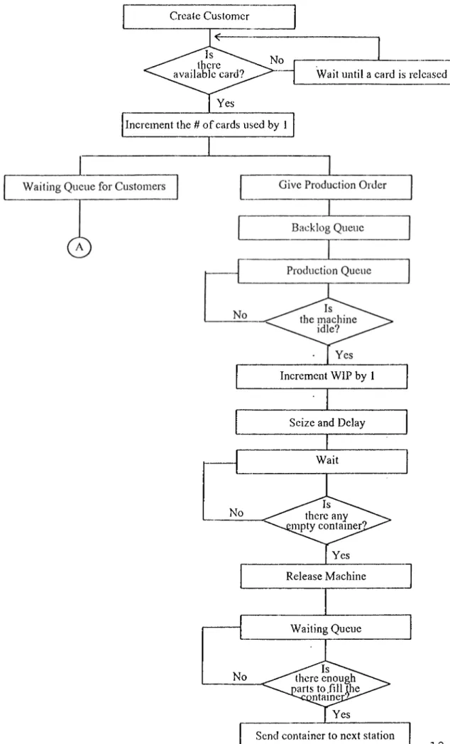
When a part leaves the last station, it is counted for measuring tliroughput and the backlog card attached to this part is freed. This backlog card becomes available to waiting customers. The part which has been finished is given to the customer and the customer demand is satisfied. The flow chart of the simulation model is presented in Figure 3.

Figure 3. Flow Chart of the Simulation Model

Create Customer

^ '\a v a ila b le Wait until a card is released

| Ye s

Increment the # of cards used by 1

Increment WIP by 1

Seize and Delay

Wait there; any )ntainer2.^--^ Yes *"\vgmpty cc Release Machine Waiting Queue X T No there c:nO U gh^\^ Jill the fv e s "^^^\narts to

Send container to next station

Flow Chart of the Simulation Model (Continued')

4.2 NOTATION

The decision variables and parameters used in the thesis are as follows;

N C n d V M D t WIP Flow number of stations container capacity

number of containers between eveiy two stations distance between eveiy two stations

velocity of a container between every two stations the number of backlog cards

demand (min/Tinit)

throughput of the production system average Work-In-Process Inventory level average flow time

4.3 ASSUMPTIONS

The Operating Assumptions o f the Production Line

• The first workstation has unlimited input available (raw materials). • No station breakdown is allowed.

• No nonconfirming unit is manufactured.

• The processing time of a part in a workstation is distributed according to a specific distribution function M'ith known parameters.

• The containers which move between workstations are standard in size. • Parts are taken out of the containers one at a time.

• The flow time of parts in the system is the sum of processing times, waiting times and transportation times of the related part.

• Containers move when they are completely filled or when they are completely empty. Partially filled containers cannot move between stations. If a workstation is busy, the other parts wait in the container to be processed.

• The number of backlog cards (M) is a decision variable.

The Mode! Assumptions

• The processing times of machines in each workstation has a gamma distribution with known parameters having a mean of 1.

• Sales arc deterministic with known parameters.

• Containers have fixed speed and the distances between workstations are given as parameters. (v=I, dl2, dl3...).

• The containers are set free and sent back to the upstream workstation when all the parts in that container are removed.

5.1 DETERMINAl'ION OF THE NUMBER OF STATIONS

To detennine the number of stations (N) to be used in this study, a set of experiments have been performed with the following parameters;

N-2,3..10 C = lan d 5

d^l unit 11= 1

V=1 unit/time D=1 min/unit

Taking the number of stations variable and other variables fixed, the results are taken for VVIP and tliroughput.

The creation of sales and processing times of machines are distributed by gamma with parameters a=25 and P=0.1 where coefficient of variation is 0.2. n is set at 1 for every container location. The results are obtained for C=1 and C=5. These results are depicted in Figures 4 and 5. 5. EXPERIMENTATION C «1 I C =5 Figure 4. 23

Figure 4 shows that as the number of stations increases, throughput of the system decreases for small values of N and stays nearly the same for larger values. It is obseiwcd that there is a decrease until N=^-6, but then the decrease in tliroughput is so small that, tliroughput stays stable.

C“1

C*=5

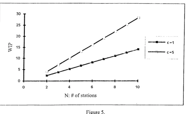
Figure 5.

In Figure 5, the behavior of WIP is plotted as the number of stations increases. As N increases, WIP also inereases. There seems a proportional relation between WIP and N. This result is an expected one, sinee if N increases, there will be more stations and more cars (containers) which results in more WIP.

From this analysis, the decision to use N^6 is made. When N is 6, in Figure 4, it enters into a region where tliroughput is stable. So in this study in all the experiments we used a 6- station serial production line.

The decision variables are C and n where the results are observed on throughput and WIP of the system. The following parameters arc used and the results arc depicted in Figures 6 and 7 .

N -6 C=I,2,5,10

d=l unit n=I,2,..6

V=1 unit/time D~1 min/unit

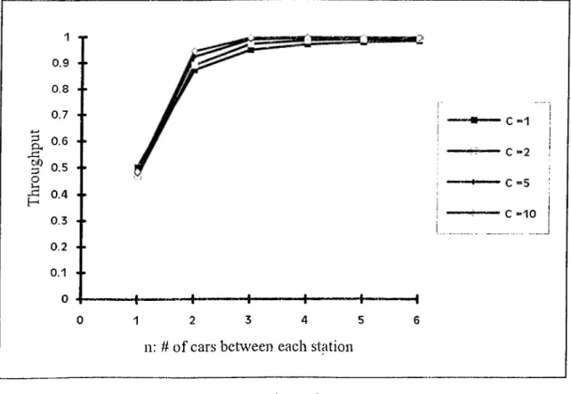
Figure 6 shows that throughput increases as n increases for different values of C. It is seen that when n increases from 1 to 2, there is a significant increase in throughput. The main point is that the increase in throughput after n=2 to n^6 is negligible. There is no need to increase n further after n=2.

5.2 ANALYSIS OF EQUALLY DISTRIBUTED CONTAINERS

1 0.9 ·· 0.8 · · 0.7 · · I 0.6 .. J=i 3^ 0.5 · · O £ 0.4 -H 0.3 - · 0.2 - · 0.1 · · 0 - — -+■ 1 2 3 4 5

n: # of cars between each station

c *=1 c «2 c =5 c « 1 0 F ig u re 6. 25

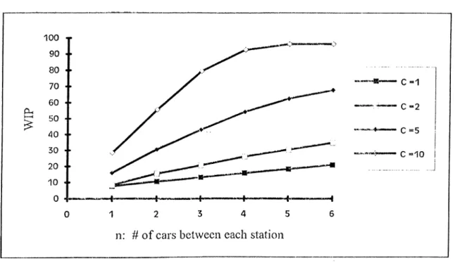
Figure 7 shows that the increase in WIP is fiister until n=3 and then the growth of WIP slows down. For some values of C, WIP stays stable after n=3. So further increase of n from 3 will not add up to WIP.

Figure 7.

The runs are made with the following parameters. The results are depieted below.

N=6 C=5

d==l unit 11^1,2,3,4

V--1 unit/time D~0.75, 1, 2, 4, 5 min/unit

From Figure 8, as demand inereases (as D decreases) up to a point, throughput increases. When demand is greater than the capacity of the system, throughput stays constant. For different values of n, the point where throughput stays constant changes. This point determines the full capacity of the system with given variables.

5.3 ANALYSIS OF DEMAND VARIATION

D“1

n=2 n * 3

n=4

Figure 8.

From Figure 9, the demand which gives the full capacity throughput, is the demand where WIP starts to be constant. As demand increases (as D decreases), WIP increases. When the system reaches full capacity, WIP stays constant.

With this analysis, from now on, I set D=-l min/iinit which is the point that makes the system work at its full capacity. The full capacity of a production line is defined as the theoretical capacity which is determined by the design of the production line.

The analysis is made for D=1 minAmit which is considered to be full demand and D= 1.2 minAinit which is considered to be low demand. The results are obtained by varying M which determines the working rate of the production system with the given parameters.

5.4 ANALYSIS OF FULL DEMAND AND LOW DEMAND

N=6 d= 1 unit V=I unit/time C-5 11= 1,2 D=1, 1.2 minAinit ■ n=1 --- n=2 Figure 10.

From Figure 10, as M increases, throughput increases to a certain level and then it stays constant. The pattern is the same for both demand levels. The difference is that, when demand is low, throughput is lower compared to the full demand. There is an upper bound on M for any given design. Further increases in M causes longer queues, but it does not have any effect on throughput.

35 30 25 CU 20 f ^ 15 ·· 10 5 0 n*=-1 n = 2 10 20 30 M: # of cards 40 •H 50 Figure 11.

From Figure 11, as M increases, WIP increases up to a point, and then stays constant. The point where WIP starts to be constant, is a critical point for M. From that critical M, further increases in M is useless. The pattern is the same for low demand. Since, in low demand, level of WIP is lower than of full demand. This is an expected result. If demand is low, the nujTiber of parts in the production line will be lower compared to the full demand case.

The analysis is performed for different values of C and M where the results are depleted. 5.5 EFFECT OF C AND M N-6 d==l unit V=1 unit/time C =l,2,5,10,20,30,40,50 n=2 D“ 1 min/unit M=10,20,30,50,100,200

For a fixed M, as C increases, throughput decreases. Since M sets the number of parts that can enter into the system, increasing C will decrease the output per unit time. While increasing C, if one also increases M, this does not affect throughput much. As M increases, the point where throughput starts decreasing shifts left, which means throughput starts decreasing in higher C values (Figure 12).

M-10 M “ 20 M = 3 0 M - 5 0 M “ 100 M “200 Figure 12. 31

For a fixed M, as C increases, WIP increases to a level where it starts to be constant afteiAvards. When the system reaches steady state, as n is 2, high values of C does not affect WIP. The value of C where WIP reaches stability is a critical point (Figure 13).

WIP vs C - M=10 M = 2 0 M - 3 0 M “ 50 M»100 M - 2 0 0 Figure 13.

For a fixed C, as M increases, throughput increases up to a point. Starting with a small value of M causes the production line to work under capacity. As M is increased, more parts enter into the system. M should be increased until no further effect on tlrroughput is observed. That is the point where throughput stays constant. That means adding more cards (increasing M) to the system will not help. The value of M at this point is critical (Figure

14).

• C =1 ! • C - 2 • C - 5 C - 1 0 C - 2 0 C - 3 0 C - 5 0 Figure 14.

For a fixed C, as M increases, WIP increases. The point found in Figure 14 is the place where WIP starts being constant. After that point increasing M further will not increase WIP and will be useless (Figure 15).

• C “ 1 • c »2 ' c - 5 C “ 10 C “ 20 C “ 50 Figu re 15. 33

Transportation time is defined as the distance between stations divided by the velocity of a container. So increasing the distance between stations means increasing the transportation time or vice versa. The parameters used in this part are as follows;

5.6 EFFECT OF TRANSPORTATION TIME

N-6 d“ l,2,3,4 unit V=1 unit/time M=200 C-1,2,5,10,20,30,50 11=2 D=1 min/unit

For a fixed C, as d increases, throughput decreases. It takes longer for containers to move from one point to another. This is an expected result. Parts spend more time in containers than they spend in workstations (Figure 16).

1 ·· 0,9 ·· 0.8 ■ · 0.7 ·· a, 0.6 ■. # 0 . 5 . . J 0.4 .. ^ 0.3 . . 0.2

..

For a fixed d, as C increases, throughput increases to a level, and reaches a peak, and starts decreasing after that point. The plot given below is a concave one. The capacity at which throughput is at its peak level is a critical point. When the curves are analyzed for different values of d, it is observed that throughput is higher for smaller values of d. As d increases, the peak level of throughput decreases (Figure 17).

d»1 d“2 d=3 d=4 Figure 17. 3 5

For a fixed d, as C increases, flow time decreases down to a critical point where it starts increasing afterwards. It has a mininuim level for a given C with these parameters. The shape is a convex one. The capacity at this point is important, since it is a guideline for the decision makers. As d increases for a fixed C, flow time increases. This is an expected result. As d increases, the time spent in the production line (by definition flow time) for each part increases (Figure 18).

d = l d=2 d “ 3 d - 4 Figure 18. 36

Varying the values of C and M, the production system shows certain characteristics. WIP and throughput are two performance measui'es of how well a production system pei forms. But for some designs, WIP and throughput are two results that contradict. Generally there must be a trade-off between them. The higher the throughput, the better. The higher the WIP, the worse. The parameters used in analyzing the trade-off are;

5.7 ANALYSIS OF WIP VS THROUGHPUT

N=6 d=l unit V=1 unit/time C-1,2,5,10,20,30 50 n=2 D=1 min/unit M - 10,20,30,50,100,200

'fhe design of a production system than must maintain the highest throughput and the lowest WIP. When these performance measures are analyzed for different values of C and M, Figure 19 is obtained.

When Figure 19 is examined for a fixed M, as C increases, throughput starts to increase to a certain level and starts to decrease afterwards. While throughput increases, WIP also increases. But, when throughput is decreasing, WIP continues to increase. There is a critical point where throughput is at its maximum point with the given WIP. This critical point differs for each different design. Then managers should look for this curve as a guideline to determine the decision variables with the highest throughput and lowest WIP.

6. CONCLUSION

I ’he design of production systems focused on either pull or push production systems. The objective of the studies made in the research literature is for improving the efficiency of these systems. Manufacturing systems generally require huge amount of investments. Knowing this, a small improvement in such systems results in considerable savings.

Any production line has several decision variables that managers have to decide about. In our production line, the main decision variables are the number of containers (n), the number of backlog cards (M), distance between statioiis (d), demand rate (D) and the capacity of the containers (C). Considering these decision variables, managers have to analyze the performance of a system with the performance measures such as throughput, WIP and flow time.

6.1 CONTRIBUTION OF THIS STUDY

The distinctive characteristic of the system considered in this thesis is that it is a CONWIP system. CONWIP systems, to the best knowledge of the author, are not applied in manufacturing much especially in Turkey. The advantage of CONWIP systems is that it includes the advantages of both push and pull systems.

'fhe main characteristics of a CONWIP system is that the number of backlog cards (M) is fixed at a point and the performance is measured with different designs. The value of M is critically important, since it sets the level of WIP of the production system. In cases of low demand, managers are free to change the value of M which changes the output rate of the production line. Decreasing M will slow down the production line, so WIP will be kept at a lower level.

6.2 RESULTS

1. When containers are equally distributed between stations; as the number of containers increases (n), throughput increases to a saturation level. At this level, n should be fixed, as increasing n further will be useless. The level of WIP at this level should be examined by the managers, since WIP costs.

2. As capacity of containers increases, WIP also increases, but throughput does not change much for n greater than 2. Increasing the number of containers from I to 2 mainly recovers the lost capacity.

3. For any real manufacturing system, the real problem is the distribution of demand. The workings of any production line is based on the demand rate. Each production line design has a theoretical weight that it can hold. So demand rate can only go up to that level. Demand that is greater than this rate will only cause longer queues in the system.

4. The demand rate that causes the system to work at its highest performance is considered as full demand. Lower rates cause the production line to work under capacity. If demand is low, relatively throughput and WIP will be lower. If demand fluctuates in time, than managers should play with the value of M w'hich will slow down or speed up the working rate of the system.

5. The decision variables C and M have considerable effect on system performance. After having fixed M, if C is increased, throughput decreases. Then the capacity at which throughput is maximum should be chosen. As M is increased, throughput

increases up to a point where it is constant afterwards. So the number of backlog cards should be set at this point.

6. Another important deeision variable in production lines is the transportation time of containers between stations. As transportation time increases, throughput decreases. So transportation time should be kept at minimum. Transportation time does not affect WIP, since WIP is bounded by the number of backlog cards.

7. The performance measures throughput and WIP generally contradict with each other. In sortie cases, there has to be a trade-off in between. The optimal performance measures should be selected so that throughput is maximized and WIP is minimized.

6.3 FURTHER RESEARCH ITEMS

Although some results have been obtained as listed above, there are several questions remaining to be addressed in CONWIP production lines. If the distribution of containers between stations are unequal, how will the above results change? If we relax the assumption that all workstations have the same processing time distribution, what will happen? There will be a bottleneck workstation which will change all system performance measures. The container sizes are standard. If containers having different capacities are used, how will they be allocated between stations? The results above are for a serial production line. What happens if there exists parallel stations that perform the same tasks? What kind of a design can be made?

APPENDIX

Begin, NO; I ■f c- A- k' k- k' k’k ' k ' k ' k - k - k - k - k - k i c - A ’k - k - k - k - k i c ' k ' k - k ' k ' k i c i c k ' k i c - k ' k ' k ' k ' k - k - k ' k - k ' k - k - k ! **** STATION # 1 ****** I * * * * * * * * * * * * * * * * * * * * * * * * * * * * * * * * * * * * * * * * * * * * * Station,1; Branch,1:

IF, A(3).EQ.O, INPUTl: ELSE, READYl;

READYl Free;

Delay : 0 : Dispose;

INPUTl Queue,1: Detach;

STANDBY Queue,2;

Scan : X(l).LT.ED(8);

!Backlog queue

! E D (8) is the capacity of a container.

PLUS Assign: X(1)=X(1)+1;

Assign: A(l)=X(1); Branch,1:

IF, A(l).EQ.ED(8), INITIAL:

ELSE, CONTINUE;

! Indexes for keeping track of entity

! transfer between stations

INITIAL Assign: X(1)=0; CONTINUE Queue,3; Scan: NR(l).EQ.O; Assign: X (7) =X (7) H-1; Queue,4; Seize: Mach i n e (1); Delay: E D (1); Branch,1:

IF, A(l).EQ.l, CONTAl: ELSE, CONTBl;

CONTAl Queue,5;

Scan : NT(1).LT.MT(l);

! Production Queue

! X(7) keeps track of # of entities in

! the system for WIP control.

1 Part is processed on Machine 1

! Check if there is an empty container

! of Typel

Queue,6;

Request,!: T R ANSI(SDS,2); ! Order a Type 1 container

! Free Machine 1

! Wait until the container is full

Release: Machine(1); Queue,7; Scan: NQ(9).GE.ED(8)-1; Branch,2: ALWAYS, SENDl: ALWAYS, DECl;

SENDl Transport: T R ANSI(A(2)),2; ! Send the container to Station 2

CONTBl Queue,8;

Scan: N Q (9).L T .E D (8)-1; ! The parts that will fill the container

Release: Machine(1);

ROOMl Queue,9; ! Dummy queue full of entities to be sent

Wait: 10, ED(8)-1: NEXT(TEMPl);

h P P

DECl TEMPI

Signal: 10, ED(8)-1: Dispose; Queue,10/

Wait: 1, ED(8)-1;

R o u t e : 0,2;

! Wait until the container is full

! Send the container to Station 2

I * * * * * * T « . * * * * * : t * * * * * * * * * * * * * * * S t * * * * * * * * · * · * * * · * · * * * I **** STATION # 2 ****** I * * * * * * * * * * * * * * * * * * * * * * * * * * * * * * * * * * * * * * * * * * * * * READY2 Station,2; Branch,1:

IF, A(3).EQ.O, INPUT2; ELSE, READY2;

Free ;

Delay : 0 : Dispose;

INPUT2 Queue,11;

Branch,1:

IF, A(l).EQ.l, SIGl: ELSE, OKEYl;

SIGl Signal:!, ED(8)-1; ! Send a signal to the wait block to

! call the parts to Station2

! Check if Machine 2 is idle

OKEYl Queue,12;

Scan: N R (2).EQ.0; Branch,1:

IF, A(l).EQ.l, G O l l : ELSE, G012;

GOll Assign: X(2)=A(2) : NEXT (WORKl) ; I Record the index of the coining

G012 Branch,!: ! container

IF, A(l).EQ.ED(8), EMPTYl: ELSE, WORKl;

EMPTYl Free: TRA N S I (X(2));

Branch,2: ALWAYS, WORKl: ALWAYS, BACKl; BACKl Queue,13 ; Request,2: T R A N S I (SDS,3); Transport: T R A N S I (A(3)),1; WORKl Queue,14; Seize: Ma c h i n e (2); Delay: E D (2);

! If the last part in the container

! is taken, then free container

! Part is processed on Machine 2

Branch,1:

IF, A(l).EQ.l, CONTA2: ELSE, CONTB2;

CONTA2 Queue,15;

Scan : N T (2).LT.MT(2);

Queue,16;

Request,!: TRANS2(SDS,2)

! Check if there is an empty container

! of Type 2

! Order a Type 2 container

h P P

SEND2

Release: Machine(2); ! Free Machine 2

Queue,17;

Scan: N Q (19).G E .E D (8)-1; ! Wait until the container is full

Branch,2:

ALWAYS, SEND2: ALWAYS, DEC2;

Transport: TRANS2(A(2)),3; ! Send the container to Station 3

C0NTB2

ROOM 2

DEC2 TEMP2

Queue,18;

Scan: NQ(19).LT.ED(8)-1; ! The parts that will fill the container

Release: Machine(2);

Queue,19; ! Dummy queue full of entities to be sent

Wait: 11, ED(8)-1: NEXT(TEMP2); Signal: 11, ED(8)-1: Dispose; Queue,20;

Wait: 2, ED(8)-1; Route: 0,3;

] Wait until thé container is full

! Send the container to Station 3

ic-k-k'k'k-k-k-k-k-kic-k'k-k-k-k'k-k'k-kic-k-k'k-k-k'k-k'k-k-k-k-k-k-k-k-k-k-k-k-k-k-k'k'k **** STATION # 3 ****** ********************************************* READY3 Station,3 ; Branch,1 :

IF, A(3).EQ.O, INPUT3: ELSE, READY3;

Free ;

Delay : 0 : Dispose;

INPUT3 Queue,21;

Branch,1 :

IF, A(l).EQ.1, S IG2: ELSE, OKEY2; SIG2 Signal : 2, E D (8) -1 ; OKEY2 Queue,22; Scan: NR(3).EQ.O; Branch,1: IF, A(l).EQ.1, G 0 2 1 : ELSE, G022;

G021 Assign: X(3)=A(2): NEXT(WORK2);

G022 Branch,!:

IF, A(l).EQ.ED(8), EMPTY2:

ELSE, W0RK2;

EMPTY2 Free: TRANS2(X(3));

Branch,2: ALWAYS, W0RK2: ALWAYS, BACK2; BACK2 Queue,23; Request,2: TRANS2(SDS,3); Transport: TRANS2(A(3)),2; h P P

W0RK2 Queue,24;

Seize: M a chineO);

Delay: ED(3); ! Part is processed on Machine 3

CONTA3

Branch,1:

IF, A(l).EQ.l, C0NTA3: ELSE, C0NTB3;

Que u e ,25;

Scan : NT(3).LT.MT(3); ! Check if there is an empty container

! of Type 3

Queue,26;

Request,!: TRANS3(SDS,2); ! Order a Type 3 container

! Free Machine 3

! Wait until the container is full

SEND3 Release: Machine(3) ; Q ueue,27; Scan: N Q (29).GE.ED(8)-1; Branch,2: ALWAYS, SEND3: ALWAYS, DEC3;

Transport: TRANS3(A(2)),4; ! Send the container to Station 4

C0NTB3

R00M3

DEC3 TEMP3

Queue,28;

Scan: N Q (29).L T .E D (8)-1; 1 The parts that will fill the container

Release: Machine(3);

Queue,29; ! Dummy queue full of entities to be sent

Wait: 12, ED(8)-1: NEXT(TEMP3); Signal: 12, ED(8)-1: Dispose; Que u e ,30;

Wait: 3,ED(8)-1;

R o u t e : 0,4;

! Wait until the container is full

! Send the container to Station 4

*★ *******************★ **********·**·)·:*·*■****■*·*** ■k*** STATION # 4 ****** * * * * * * * * * * * * * * * * * * * * * * * * * * * * * * * * * * * * * * * * * * * * * RE7\DY4 Station,4; Branch,1:

IF, A(3).EQ.O, INPUT4; ELSE, READY4;

Free ;

Delay : 0 : Dispose;

INPUT4 Queue,31;

Branch,1:

IF, A(l) .EQ.l, SIG3 ; ELSE, OKEY3;

SIG3 Signal:3, ED(8)-1;

OKEY3 Queue,32; Scan: N R (4).EQ.O; Branch,1: IF, A(l).EQ.l, G031; h P P

G031 . Assign: X(4)=A(2): NEXT(W0RK3);

G032 Branch,!:

IF, A(l).EQ.ED(8), EMPTY3:

ELSE, W0RK3;

EMPTY3 Free: TRANS3(X(4))/

Branch,2:

ALWAYS, W0RK3:

ALWAYS, BACK3;

BACK3 Queue,33;

Request,2: TRANS3(SDS,3); Transport: TRANS3 (A(3)),3;

ELSE, G032;

W0RK3 Queue,34;

Seize: Machine(4);

Delay: ED(4); Part is processed on Machine 4

Branch,1:

IF, A(l).EQ.l, C0NTA4: ELSE, C0NTB4; C0NTA4 Queue,35; Scan : NT(4).LT.MT(4); Queue,36; Request,!: TRANS4(SDS,2) ; Re!ease: Machine(4); Queue,37; Scan: NQ(39).GE.ED(8)-!; Branch,2: ALWAYS, SEND4: ALWAYS, DEC4;

SEND4 Transport: TRANS4(A(2)),5; ! Send the container to Station 5

! Check if there is an empty container

! of Type 4

! Order a Type 4 container

! Free Machine 4

! Wait unti! the container is full

C0NTB4

R00M4

DEC4 TEMP4

Queue,38;

Scan: N Q (39).L T .E D (8)-1; ! The parts that will fill the container

Release: Machine(4);

Queue,39; ! Dummy queue full of entities to be sent

Wait: 13, ED(8)-1: NEXT(TEMP4); Signal: 13, ED(8)-1: Dispose; Queue,40;

Wait: 4, ED(8)-1;

R o u t e : 0,5;

! Wait until the container is full

! Send the container to Station 5

**·)!: yr***i»r*-A ***-*****'A-*****-**************T^ ******

**** STATION # 5 ******

*'**★ **★ VI'**·*·*·*·*** Alt *****★ *·**·*■***★ ****** ****Vt·**

Station,5; Branch,1:

IF, A(3).EQ.O, INPUTS: ELSE, READY5;

h P P

READY5 Free ;

^ Delay : 0 : Dispose;

INPUTS Queue,41;

Branch,1:

IF, A(l) .EQ.1, SIG4 ; ELSE, OKEY4;

SIG4 Signal: 4, ED(8)-1;

0KEY4 Queue,42;

Scan: N R (5).E Q .0; Branch,1:

IF, A(l).EQ.1, G 0 4 1 : ELSE, G042;

G041 Assign: X(5)=A(2): NEXT(W0RK4)

G042 Branch,!:

IF, A(l).EQ.ED(8), EMPTY4:

ELSE, W0RK4; EMPTY4 F r e e : TRANS4(X(5)); Branch,2: ALWAYS, W 0 R K 4 : ALWAYS, BACK4; BACK4 Queue,43; Request,2: TRANS4(SDS,3); Transport: TRANS4(A(3)),4; W0RK4 Queue,44; Seize: Machine(5);

Delay: E D (5); ! Part is processed on Machine 5

CONTAS

SENDS

Branch,1:

IF, A(l).EQ.l, CONTAS: ELSE, CONTBS;

Queue,4S;

Scan : NT(S).LT.MT(S); ! Check if there is an empty container

! of Type S

Queue,46;

Request,!: TR7\NS5 (SDS, 2) ; ! Order a Type S container

! Free Machine S

! Wait until the container is full

Release: M a chine(5); Queue,47; Scan: NQ(49).GE.ED(8)-1; Branch,2: ALWAYS, SENDS: ALWAYS, DECS;

Transport: TRANSS(A(2) ) ,6; ! Send the container to Station 6

CONTBS Queue,48;

Scan: N Q (49).L T .E D (8)-1; ! The parts that will fill the container

Release: Machine(S);

ROOMS Queue,49; ! Dummy queue full of entities to be sent

Wait: 14, ED(8)-1: NEXT(TEMPS);

DECS Signal: 14, ED(8)-1: Dispose;

TEMPS Queue,SO;

h P P

Wait: 5, ED(8)-1;

Route: 0 , 6 ;

! Wait until the container is full

! Send the container to Station 6

*·*·**** + ★ ************★ ***********·*·*■*·********** **** STATION # 6 ****** ********************************************* Station,6; Queue,51; Branch,1: IF, A(l).EQ.1, S I G 5 : ELSE, 0KEY5;

SIG5 Signal: 5, ED(8)-1;

0KEY5 Queue,52;

Scan: NR(6).EQ.O;

Branch,1:

IF, A(l).EQ.1, G 0 5 1 : ELSE, G052;

G051 Assign: X(6)=A(2): NEXT(W0RK5);

G052 Branch,!:

IF, A(l).EQ.ED(8), EMPTY5:

ELSE, W0RK5;

EMPTY5 Free: TRANS5(X(6));

Branch,2: ALWAYS, V70RK5: ALWAYS, BACK5; BACK5 Queue,53; Request,2: TRANS5(SDS,3); Transport: TRANS5(A(3)),5; W0RK5 FG Queue,54; Seize: Machine(6); D e l a y : E D (6); Release: Machine(6); Assign: X(7)-X(7)-l; Queue,55 : Detach;

Part is processed on Machine 6

F r e e Machine 6

Decrease # of entities in the system by 1

! Finished Goods Inventory

I *** *****************************************

I ***** SALES *****

I ******************************************** h

P P

SALES Create,1,0: ED(7); Branch,3:

! Creates the sales

Always, BACKLOG: ! Entity sent to BACKLOG queue

Always, SOLD: ! Copy of the entity sent to SOLD

Always, PRODUCE; ! Copy of the entity sent to PRODUCE

BACKLOG R o u t e :0,1; ! Send part to Station 1

SOLD Branch,1:

IF, NQ(55).GT.O, SOLDI: ! Normal Sales

ELSE, LOST; ! Lost Sales

SOLDI Remove: 1, 55, SELL: Dispose; ! Part taken out of F G I , then SELL

LOST Count: 1, 1: Dispose; ! Nuinber of Lost-Sales

PRODUCE Remove: 1, 1, STANDBY: Dispose; ! Part is sent to production

SELL Count: 2, 1: Dispose; ! The number of units sold

I • k - k ' k ^ - k ' k - k - k - k - k ' k - k - k ' k - k - k - k - k - k - k ' k - k E n d O f S3.1 0S * * * * * * * * * * * · * · * * * * · * * * * · * * * * *

End;

h P P