ESTIMATION OF VELOCITY FUNCTION FOR TURKEY USING ENGLE-GRANGER TWO-STEP METHOD
A Thesis
Submitted to the Department of Economics and the Institute of Economics and Social Sciences
of Bilkent University
In Partial Fulfillment of the Requirements for the Degree of
MASTER OF ARTS IN ECONOMICS
By
Murat Ali YÜLEK November, 1990
f f G
Z Z Q . Ç
Ів'Эо
I certify that I have read this thesis and in my opinion it is fully adequate, in scope and in quality, as a thesis for the degree of Master of Arts in Economics
Prof. Dİv Süb:í«ey Togan
I certify that I have read this thesis and in my opinion it is fully adequate, in scope and in quality, as a thesis for the degree of Master of Arts in Economics
Assoc. Prof. Ümit Erol
I certify that I have read this thesis and in my opinion it is fully adequate, in scope and in quality, as a thesis for the degree of Master of Arts in Economics
f
_ L L £ İd j± k > .
Assoc.Prq^ Erine Yeldan
I would like to thank Prof. Dr. Subidey logon for leading me to this study and for his encouragements and recommendotions during the preparation of the study. I also wish to thank to Dr. Ahmet Ertugrul and Dr. Osman Zaim for their involuable help.
I should also thank Ismail Arslan and Zeynep Ada of SPO and Fotih Özatay of CB of Turkey and Şebnem Akkaya of WB for providing with data and consultations. I should not forget dear classmates Erdem Başçı, Süheyla Özyıldırım and Jülide Yıldırım for their invaluable comments.
I wish to express my gratefullness also to Alaettin Eğribaş, Seher Öztürk, Bilge Akpınar, Sezgin Özyıldırım, Murat Erker and Sema Bakkaloğlu who, with unbelievable patience had to read my handwriting and helped me with the typing work.
ACKNOWLEDGEMENTS
Finally my thanks are extended to my family who provided me comfortable environment and encouraged me during the preparation of thesis.
ABSTRACT
ESTIMATION OF VELOCITY FUNCTION FOR TURKEY USING ENGLE GRANGER TWO-STEP METHOD
Murat All YULEK MA in Economics
Supervisor: Prof. Dr. Siibidey Togan
November 1990, 47 Pages
This study aims at estimating the velocity function, for
Turkey using quarterly data. Estimation is done using
cointegration and error correction methods. This enabled
incorporating short-term disequilibria moments in long run equilibrium.
The analysis starts with examination of level of integration of series in question. Then a number of cointegrating regressions are run. Cointegrated series are employed in different "lag-rich"
error correction formulations. Finally using a general to
specific approach, parsimonious models are reached dropping insignificant regressors.
Key words Cointegration, level of integration, stationarity,
error correction model, reparameterisation, adaptive Expectations, auto-regressive distributed lag model, vector auto-regression.
ÖZET
HIZ f o n k s i y o n u n Tü r k i y e Iç î n e n g l e-g r a n g e r IkI-b a s a m a k l i METODUYLA TAHMiNl
Murat Ali Yülek Yüksek Lisans Tezi
Ekonomi ve Sosyal Bilimler Enstitüsü Tez Yöneticisi: Prof. Dr. Sübidey Togan
Kasım 1990, 47 Sayfa
Bu çalışmada Türkiye için 3 aylık veriler kullanılarak hız
fonksiyonunun tahmin edilmesi amiıçlarımaktadır. Tahminde, eş-
bütünleşme (cointegration) ve hata-düzeltme (error correction)
yöntemleri kullanılınıştır. Bu yöntemlerin ana özelliği uzun dönem
denge yapısını saklı tutarken, kısa dönem sapmalarını
açıklayabilmeleridir.
Analize, kullanılan veri dizilerinin bütünleşme derecele
rinin (level of integration) test edilmesiyle başlanmaktadır.
Bundan sonrci eş-bütünleşme regresyonlar ı (cointegrating-
regressions) yapılmakta ve eş-bütün seriler değişik hata-düzeltme
modellerinde denenmektedir. Başlangıçta, zengin bir gecikmeli-
değişken yapısına sahip alan modeller genelden-basite yaklaşı mıyla önemsiz değişkenler atılarak basitleştirilmektedir.
TABLE OF CONTENTS I . ACKNOWLEDGEMENTS ABSTRACT OZET INTRODUCTION
II. THEORETICAL BACKGROUND
1. Money Demand Functions
2. Derivation of Expected Loss Term
3. Cointegration any Error Correction Methods
3.1. Integration, Stationary and Nonstationary
Series
3.2. Cointegration
3.3. Error Correction and Cointegration
3.4. A Digression : Auto-regressive,
Distributed Lag Models (AD) and ECM 3.5 Engle-Granger two-step Method
3.6. Empirical Estimation Procedure
3.7. Construction and Estimation of EC Models 3.8. Validity Tests 2 2 5 6 6 9 10 12 14 15 19 19
III. EMPIRICAL STUDIES ON ESTIMATING VELOCITY FUNCTIONS USING EC METHODS
1. Determination of Level of Integration 2. Testing For Cointegration
3. EC Formulation of the Model 4. Evaluation of Approaches 22 22 23 26 36
IV. CONCLUSIONS AND RECOMMENDATIONS FOR FURTHER STUDY
V. REFERENCES
VI. DATA SOURCES AND DATA MATRIX
38 40 42
LIST OF TABLES
1 . Main Characteristics of 3 (0) and I (1) series 8
2 . Critical Values for ADF , DF and CRDW Tests 18
3. DF and ADF Statistics for the Series 22
4. Cointegrating Regressions 25
5. Estimation Results for the First Approach 27
6 . Unrestricted Dynamic Model for the First Approach 29
7. Estimation Results for the Second Approach 31
8 . Diagnostic Test Results for the Second Approach 32
9. VAR Estimates 33
10. Estimation Results for the Third Approach 35
I. INTRODUCTION
This study is devoted to the estimation of velocity function under broad and narrow definitions of money (Ml, M2) for Turkey, using Error Correction Methods.
The study first covers theoretical background of
velocity functions and Error Correction Methods that are employed. Then results of empirical estimations are reported. In
r
the study, a Cagan type money demand function that constitutes the basis for the velocity function which is estimated, is used. This, with certain modifications, led to a velocity function which had Income and Expected Loss (which in this study is the name used for minus of real interest rate) as the arguments. Expectations are assumed to form adaptively.
Estimation is made using Engle-Granger two-step method. In
this approach, first a cointegrating regression is run. Then,
assuming non-cointegration is rejected, residuals from this
regression is used as error correction term in an appropriate
error-correction model.
The organisation of the study is as follows: In the first section, theoretical background - namely derivation of velocity
function, expectation formation and error correction methods-
is briefed. Second section presents the empirical findings and results of diagnostic tests. Conclusions and recommendations for further study closes the thesis.
II. THEORETICAL· BACKGROUND
1. Money Demand and Velocity Functions
The question of demand for money had been an ever-fresh topic for many researchers and theorists. To answer the question: why do people hold money balances? or put in a different way,what are the determinants of demand for money?, extensive empirical study has been done. However the subject is still a domain of substantial discussion.
Very briefly three main questions that still are under severe discussion are (*):
1 ) constraint that is imposed on money balances:
- whether the appropriate constraint is wealth, income or a combination of the two.
2 ) importance of interest rates and price changes as
arguments in the demand function.
3) definition of money to be used.
In this study, we don't want to get deeply involved in the discussions between different schools and instead follow a practical way to reach the velocity function which will be estimated.
In a standard Cagan type money demand function which has is extensively used in empirical studies and whose theoretical consistency has been proved, main arguments are real income (y) and expected inflation (n) :
D D
M b -c M
--- = k y e or Ln (--- ) = a + blny - c ... (1)
P P
where k = e^
The presence of expected inflation term in such a function is validated by the idea that, alternative cost of holding money
in periods of rapid inflation, is simply expected price
increases. We proceed however by modifying the above function by;
D D
M b -cEL M
---- = k y e or Ln (--- ) = a + blny - cEL ... (2)
P P
Here EL is used for "Expected loss" by which we mean:
E L = r t - r ... (3)
where r is the nominal rate of return available from holding
money (net of tax), r is naturally different for different definitions of money. The calculation to obtain r will be explained in the next section. As seen easily, EL is simply the minus of real interest rate.
From celebrated quantity theory which relates velocity to nominal income through money supply :
M®v = py PY s M where : s M : money supply V : velocity p : price level y : real income (4) (5)
Now if we keep the assumption of equilibrium in money market
and hence replace with we will obtain.
py
V = (6)
M
Plugging in, what we have from our money demand equation, we reach : V = b -cEL k y e 1 (1-b) cEL ---- y e (7)
Reparameterising this last relation will yield
... (8 ) /3
V = A y ' e
and
This is the main model to be estimated in our study. However, as cointegration methods will be employed, different versions of (9) will be tried. (In this study VI denotes velocity when Ml is used as money definition and V2 that for M2 namely, Vl=Py/Ml and V2= Py/M2)
2. Derivation of Expected Loss Term
The Expected loss term consists of two components: expected inflation ('h ) nominal rate of return available from holding money
(net of tax).
Expectations of inflation are supposed to form adaptively, adjusting to the difference between the rate of inflation and expected rate of inflation in the previous period.
In Togan (1987) this type of expectation, formation was fund to be preferable to alternative types, for Turkish data. The assumed adoptive expectation scheme can be formulated as follows (*)
n-f = n.^., +p(pt-i -fif.jJ p , ^ ]n p , - In p t-1 where p represents rate of inflation
and In p natural logarithm oh the price level
Working out the mathematics will yield : t-f
' h = P : ( i - p ) + P Z P t - H 1=0
at an instant t, where Pq denotes the inflation rate at t=0 has
the limiting values (0,1). When B equals 1 the scheme becomes
naive in the sense that expectations at a period equals the actual inflation rate at previous period (*).
Next the real rate of return available from holding money is calculated for Ml and M2 in the following manner :
Tdd DD Ml: Th -m ( l - T ) M 2 : r,,-= rooC'D+r>r,TD l-t where DD TD T — i l - T ) M2 Demand Deposits Time Deposits
Tax rate on Interest Income
(In the above calculations, certificate of Deposits and Deposits at the Central Bank are not considered.)
3. Cointegration and Error Correction Methods
3.1. Integration, Stationary and Nonstationary Series
A recent contribution of Granger and Engle to the Error
Correction literature is the celebrated relation between
cointegration and error correction representations.
This relation takes its root from the theoretical-yet practically evidenced idea that certain pairs of series should be converging in the long run. Examples to these can be commodity prices in two countries open to trade or prices and wages in a country. The use of cointegration techniques applied to such
(*) For a discussion on stability considerations of this scheme see Togan (1987), pp.l587
series first necessitates the explanation of basic time series definitions.
A single stationary time series with stochastic components has an infinite moving average representation as states Wald's theorem. This representation can generally be approximated by finite autoregressive moving average process. However, most of the economic time series are not stationary. Following is the celebrated integration definition by Granger :
Definition 1 (Integration): A series with a deterministic component which has a stationary, invertible ARMA representation after differencing d times is said to be integrated of order d, denoted x^. f>j I (d ) .
For d=0 the series is stationary and for d=l the change is stationary. A time series like :
Xt = M , Xt-I ^ 02 ^M-2 ^ ■*■00 '^t-n ^ ... ( 1 )
is either stationary or non-stationary. The latter is further
subdivided into an explosive process or a unit root process. A familiar example to unit root processes is random walk process, which can be represented as follows:
X = x + e
t t-1 t
The niitin characteristics of 1 (0) and I (1) processes are as follows : (duplicated from YOSHIDA 1990)
TABLE : 1
Attrit>utes of 1(0) series Attributes of I d ) series
Fluctuate irregulatjy around
and frequent] V' intersect
tliG'ir mean.
oinct’ the effect of a sl)Ock (uj ) in ciac li period wealaMis over tinie, I(0) varialiles do not d i verge far from their mean or trends.
The mc'an x and variance s'"
calculated from observed
data are unbiased and
consistent estimators of the
true mean and variance.
Relatively accurate estimates
of coefficients can be
estimated by applying an
ordinary regression. The
estimates are known to follow a t-distribution.
Tend to have widc-'r swings. As
sample size increase,
probability of tlieir
re turning to tfie same value
appr oaclies zero.
At Ic^ast prat t of sfiot k in
G'ach quart CM ha£'
long-lasting effects : ^
X .
2
e.o i=l ^
X = X + e
t (t-1) t
Average x and variance s ,
calculated from observed data are often biased. (When T ->ir>
random walk has neither
particular mean value nor
finite variance)
In small samples, a regression
including 1(1) variables may
well yield very erroneus
results. Estimates are often biased, (cointegration is an
exception and they do not
follow a t-distribution.
As is stated in table 1, wtien a regres^sion involves one or
more I (1) series, the statistics like coefficient of
determination or t values no longer have simple text t»ook
distribution in majority of cases and tliey lead the
econometrician to incorrect inferences. It is only possible for
population mean and variance. Therefore conventional methods of estimation will lead to incorrect estimates when applied to one or more I (1) series. This fact which has long been known in statistics could gain practical importance only after Dickey- Fuller (1979) who introduced first tests to be used to determine the degree of integration of series.
3.2. Cointegration
Second familiar definition comes below : (Granger 1981)
Definition (Cointeqration): The components of the vector
are said to be cointegrated of order d, b, denoted I (d,b) if
(i) all components of x^ are I (d)
(ii) there exists a vector a (/0) so that , Zt, = ~ I (d~b), b>0
The vector ot is called the co-integrating vector.
Much of the literature concentrate on the case where d=b=l in which case, components are integrated of order 1 and error is
white noise. If such has zero mean, it will frequently cross
zero line and will not drift too far from it.
If x^ has N components such that N>2, becomes a
3.3. Error Correction and Cointegration
Error correction mechanisms have been used widely in economics. Early examples are Sargan (1964) and Phillips (1957). Currently, the studies on the subject are gradually shifting towards the utilization of cointegration methods in estimating models in a manner that is theoretically discussed in this section.
Error correction per se says that the disequilibrium in one point in time is gradually corrected. Excess supply of a certain crop this year might for example be the result of the balance last year. Successful application of the method are inter-alia DHSY (1978), Hendry and von Ungern-Sternberg (1980), Currie
(1981), Dawson (1981).
These models make use of rich lag structures including lagged dependent variables to capture true dynamic structure of the model. As a more general model they intrinsically include the long-run equilibrium while allowing short-run disequilibria, like classical econometric models. Error correction models use economic theory in assigning the components of the model.However they incorporate a rich lag structure which is not the case for the classical econometric models.
Definition 3 (Error Correction Representation, Granger,1987)
A vector time series representation x^ has an error correction representation if it can be expressed as :
A ( B ) ( 1- B ) X| =
Where = Stationary multivariate disturbance
A (B) is such that A(0)=I, A(l) has all elements finite, and by rearrangement, older lags of the error term (z) can be shown to appear as explanatory variables.
Following theorem without proof which appeared in Granger (1983) establishes the required relationship between error correction mechanisms and cointegration :
Theorem 1, Granger Representation Theorem:
Let be such that all (N) components are 1(1) so that
change in each component is zero mean, purely stochastic stationary process. Then the following will be the multivariate Wald representation of the system :
(1 - B) Xf = C(B) C (1)
which should be taken to mean that both sides will have the same spectral matrix.
If X-j- is cointegrated with d=b=l with co-integrating rank
r, then:
(1) C(l) is of N-r
(2) There exists a vector ARMA representation
A (B) Xt = d(B) ... (2)
with the properties that A(l) has rank d(B) is a scalar log
polynomial with d(l) finite and A(0) = When d(B) =1, this is
a vector autoregression.
(3) There exist Nxr matrices, |i; cv. of rank r such that,
a (1) ro C{1)>* = 0 A ( n = ^ a '
(4) There exists an error correction representation with y^5n rxl vector of stationary random variables:
= -d(B)ct... (3)
with A* (0) =
} The vector is given by:
Zt= K ( B ) i - t... (4)
0-B)Ztr ... (5)
where K(B) is an rxN matrix of log polynomials given by ♦
• C (B) with all elements of K(l) finite with rank r, and .def
> 0 .
(6 ) If a finite vector autaregressive representation is ible, it will have the form given by (2) and (3) above with
A
)=1 and both A(B) and A (B) as matrices of finite polynomials.
3.4. A Digression: Auto-Regressive Distributed Lag Model (AD) and ECM
Let's briefly denote simple univariate AD, Partial Adjust ment. Distributed Lag, and Autoregressive models:
A simple AD Model=
t- P o+P 1·"· t- ¿J t * P zy t- LI t...i 1)
Now imposing the restriction p3=0 we pass to a simple
Partial Adjustment Model=
.(
2)
Next, imposing = 0 to (1), we have a simple distributed
lag model=
^•t=Po+p2yt''-p3yt-i"‘Ut.(3)
Finally, imposing p^ = = 0 we have a first order Auto
regressive Model=
'^t=Po+Pr<t-i+Llt.(4)
As seen, AD model can be considered as a general model which has - as special cases-other 3 models,·»
Following simple but effective lines in Yoshida (1990), ECM is established from an AD model via " reparameterisation" as follows=
let: p, = 1+a, = b, 5'^ = -(b+ka)
so that (1 ) takes the form
x^3p/h;! + a ) x t _ i + D y t + ( a k + t ) ) y t - i - ^ ' - i t
and subtract x^-i from both sides to have after rearrangement.
“ •"'t-Po'^P'^yt^^L^'t-i .(6 )
The term ^t-l “ ^^t error correcting term. It is
said that in the log-run, ^t-l “ ^i^t-1 = 0 so that the equilibrium is restored. However a certain proportion of error EC^, which is=
ECt = Xt - kYt
is corrected at time instant t+1, at times of disequilibrium. By doing this, EC Model becomes a dynamic model allowing for disequilibrium, at times and equilibrium at others. The ECM representation (6 ) is a linear transformation of AD Model, therefore it shares the characteristics of AD Models.
3.5. Engel-Granger two-step Method In a regression like=
.(7)
if one or more 1 (1 ) variables are used, the regression is considered as spurious. However, Stock (1987) prooved that if
and are cointegrated, estimates of coefficients in (7) is far
more precise than an ordinary LS estimation. The reason is that in an ordinary LS estimation between 1(0) variables, convergence of coefficients to their true values is realized only at larger
samples. However when two or more cointegrated 1(1) series are
regressed, convergence is maintained even at small sample sizes.
This phonemenon is called " super-consistency". For proof one
can refer to Stock (1987).
Two step method of Engel and Granger utilizes super consistency to acliieve consistent estimates. The method proceeds as follows:
1) Using the " cointegrating regression",
an estimate found. Then Error Correction Term (EC) is calculated:
ECt=x,-p,yrPo
2) The ECM is estimated in an equation like:
/tA jiy t+A2EC^_i +u^
As can be seen by careful eyes, EC is simply the residuals from cointegrating regression.
3.6. Empirical Estimation Procedure
The estimation procedure that is employed in this study consists of three stages:
1) Testing the level of integration of series 2) Testing for cointegration
3) Construction, estimation and Testing the EC models.
Testing for level of integration:
To test level of integration ADF and DF tests were used: The two tests proceed as follows:
DF Test:
In original DW test following regression is run:
where t is trend.
Then‘S is compared with provided critical values, with / s e ( c v )
Ho: random walk. However a simpler version without any difference in the characteristics of the test is running the following:
and comparing p directly with the critical values.
Null hypothesis is taken as non-stationarity of the series, if t value for pexceeds critical value in the table. Ho is rejected, thus supporting a trend-stationary process.
..._ 1 /
ADF Test:
Following ADF regression is run: 4
i=1
The estimate ct is than compared with the critical values provided in the previous section.
Testing For Cointegration:
In line with Granger (1987) following tests can be used to test cointegration between series:
CRDW Test:
DW statistic of cointegrating regression (Cointegrating Regression DW-hencefortjth CRDW) is compared to the CRDW critical values, which are provided at the end of the section :
N yt= 2 i=l
where N is the number of total cointegrated variables minus 1
and Xj^ are cointegrated variables to y^.
The null hypothesis is taken as follows:
Hc3 - n o n - c o i n t e g r a t i o n
If the CRDW exceeds critical value, Ho is rejected, in favour of cointegration:
DF Test:
The residuals from cointegrating regression are regressed
a s :
The minus of estimate q is compared to critical values
which are provided at the end of the section.
ADF Test:
The residuals are regressed as: 4
The minus of estimate ^ is than compared to the critical
values with H o :non-cointegration. If ADF statistic exceeds
critical value. Ho is rejected in favour of co-integration.
TABLE : 2
Critical Values for ADF, DF and CRDW Tests
2 variable Case 1 % 5 % 10 % CRDW 0,511 0,386 0,322 DF 4,07 3,37 3,03 ADF 3,77 3,17 2,84 3 Variable Case 1 % 5 % 10 % CRDW 0,488 0,367 0,308 ADF 3,89 3,13 2,82
The first table is duplicated from Granger and Engel (1987) whereas the second from Hall (1986) who obtained it upon request, from also professor Granger.
All three tests are built on Monte-Carlo studies.
There are discussions on whether to include a trend and constant in the regression. In our study we contend with ADF and DF tests without a trend and constant.
3.7. Construction and Estimation of EC Models
As the cointegration regression in the following form is run: y t=c+c·;, 1{ + f X 2 ^ 2 J . ^
detecting cointegration, an EC model can be constructed
tentatively in the followinq manner:
N N N
i=0 i=u i=1
where EC represents residuals from cointegrating-regression.
n should be determined tentatively but for the case of quarterly data, n= 4~ 6 is said to be sufficient unless important explanatory variables are omitted.
The insignificant regressors are then dropped with a general- to-simple approach. Gradual reduction of number of explanatory variables also involves checking of residual autocorrelation and other testing criteria which will be considered in the next section.
3.8. Validity Tests
There are a number of tests used to check the validity of models in this study. The resulting test values are reported together with the critical values. The theoretical aspects of there tests are explained briefly in this section. All of the tests to be mentioned below are provided by PC-GIVE including the critical valves.
1. Goodness of Fit=
2. DW
The DW test which is most useful when testing white noise
against random walk residuals is biased towards 2 , when lagged
dependent variables are used as explanatory variables; hence
towards not detecting autocorrelation. In the cai;‘e where lagged
dependent variables are used as regressors, Durbin's h test or LM test are recommended.
3. LM Test:
th
The Lagrange-Multiplier Test for r^“ order auto-correlation
is distributed as (r) in large sample. Ho is taken as no
autocorrelation. In PC Give F-Form (Harvey (1981) ) is used as test statistic. Nevertheless, in our study DW statistic is reported.
o
41.
4. Normality A (2) Test: (Jargue and Bereu, 1980)
This test is employed against normality of residuals in line with J., and B.(1980). The statistic follows a X distribution with two degrees of freedom under the null hypothesis of normal residual distribution. If statistic exceeds the critical value
(which is 5,99 at a =0,05) normality is rejected.
5. Heteroscedasticity : 2
X F ) is a test statistic for residual heteroscedasticity developed by White (1980).It follows an F distribution of(2k-2,T-
3k+l ) degrees of freedom under the null of homoscedasticity,
where T is the number of observations and k is the number of
explanatory variables excluding constant term. If F-statistic
exceeds the critical value, homoscedasticity is rejected.
6. CHOW Test:
Familiar Chow Test (Chow, I960)· has been developed to test parameter constancy. It aims at detecting structural change or significant changes of coefficients between residual variance of the sample period and that of forecast period. The test statistic CH follows an F distribution with (n, T-k ) under the
null of no structural change ( T = number of observations,
k = number of eplonatory variables, n= length of out-of-sample period).
III. EMPIRICAL· STUDY ON ESTIMATION OF VSEOCITY FUNCTIONS
1. Determination of Devel of Significance
To determine the level of integration of the series in question which is the first step in the estimation of velocity
function using Engle Granger Two-step Method, ADF and DF
regressions without a constant and trend were run. Next, to reinforce our inferences, ADF and DF regressions were run for the differenced series. Results are tabulated below.
TABLE : 3
DF and ADF Statistics for the Series
Series DF ADF In y -0.30 -2,76 In vl -0,11 -0,01 In v2 1,70 1,81 Ain y 6,07 23,40 Ain vl 5,58 5,91 Ain v2 5,65 3,79 EL(M1, 13=0.3) 1,76 1,76 AEL(M1, 13=0.3) 7,29 7,87 EL(M1, B=0.5) 2,04 2,34 a e l(m i. 13=0.5) 6,29 4,72 EL(M1, 13=1.0) 2,66 2,83 AEL(M1, 13=1.0) 4,88 4,88 EL(M2, 13=0.3) -0,72 -0,06 AEL(M2, 13=0.3) 3,91 3,20 EL(M2, B=0.5) -0,36 0,17 aEL(M2, 13 = 0.5) 4,10 3,68 EL(M2, B=1.0) 0,38 0,48 AEL(M2, 13=1.0) 5,93 6,39 Here:
Vl = Py / Ml . , when Ml is used as monetary base
V2 = Py / M2 . , when M2 is used as motetary base
EL(Mi, 13-1) . loss when Mi (i=l,2) is used and
coefficient of adaptation is 1 ,
From table (3) it is clearly seen that series Iny, Invl and lnv2 are all 1 (1 ) as the levels are non-stationary and first differenced series are stationary. For these series, plottings of series also support non stationarity.
The expected loss series also present evidence for non-
stationarity. However the plottings of series for Ml are dubious.
This can be the result of lack of power of tests as approaches
1. We nevertheless consider both cases (stationarity and non- stationarity) when doing our empirical analysis in the next section.
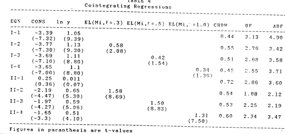
2. Testing for Cointegration
The two main cointegrating regressions that were in question were that involving Invl and Iny and that involving lnv2 and Iny. However, as the possibility of non-stationarity of expected loss series also existed, the following cointegrating regression were run : I - Narrow Money : 1 In VI = t a + /3 In y t 2 In VI = t a + 13 In y + t iEL Ml,13=0.3 3 In VI = t a + B In y + t iEL Ml,13=0.5 4 In VI = t a + 13 In y + t iEL M1,B=1.0 23
II - Broad Money : II - 1 * In V2 = a + J3 In y II - 2 In V2 = t II - 3 In VI = t II - 4 In VI = a + 13 In y + YEL t M2,13 = 0.3 a + 13 In y + YEL t Ml,13 = 0.5 a + S In y + i'EL t M1,B=1.0
The coefficients, CRDK’, ADF and DF statistics are reported
in Table (4).
All of the regressions pass CRDW test, however II-2 and II-3 fail in both DF and ADF tests, therefore they are considered as
non-cointegrated. In 1-3 and 1-4 coefficients of expected loss
series, and in II-l all of the coefficients are insignificant.
The relations which have no problem in providing healthy test statistics and significant coefficients are I-l, 1-2 and II- 4. In 1-2 and II-4 DF statistic fails however both CRDW and ADF tests provide supporting evidence in favor of cointegration and
consequently the null of non-cointegration was considered as
rejected.
TABLE 4 Cointegrating Regression: to LP EC?: CONS In y I-l -3.39 1.05 (-7.32) (9.39) 1-2 -3.77 1. 13 (-7.30) (9.30) T-3 -3.69 1.11 (-7.10) (8.80) 1-4 -3.65 1 . 1 (-7.00) (8.80) II-l 0.25 0.011 (0.36) (0.07) II-2 -2.19 0.65 (-4.47) (5.30) II-3 -1.97 0.59 (-4.27) (5.06) II-4 -1.65 0.51 (-3.3) (4.10)
EL(Mi,f .3) EL(Mi,i'-.5) EL (Mi, =1.0)
0.58
(2.0 8)
1.58
(8.6 9)
Figures in paranthesis are t— values
0 . 4 2 ( 1 . 5 4 ) 1 . 5 0 ( 8 . 8 3 ) 0 . 3 4 (1.3G) 1 . 3 1 ( 7 . 5 0 ) ROiy DF ADF — — 0.44 3.13 4.90 0.55 2.76 3.42 0.51 2.68 3.58 0.45 2.55 3.71 0.72 2.06 3.60 0.54 1.88 2.12 0.53 2.25 2.19 0.60 2.34 3.47 — — --- ---======= — — — ——
3. EC Formulation Of the Model
In this study, three approaches to tackle the problem of Error Correction Formulation have been adopted. The description of these three approaches and the estimated models are reported below:
1) Ordinary General-to-Specific Approach :
In this approach, for each of the successful
cointegration relations developed in· the previous section, a simple, lag-rich model was adopted. The change of dependent variable was regressed on four lags of each cointegrated variable and dependent variable and also of Error Correction term which is simply the residuals from cointegrating regression. The results are presented in table (5).
TABLE : 5
Estimation Results for the First Approach
EQN ¿ I n V 1 ^ = u .002-‘ u.&6 ¿ I n y ^ + 0.3 4¿ I n y y_3 (0.2'7) ( 16.5) (6.17) - 0.24 E C , . , ( -3.44) ¿ I n V 11 = -0.012+0,22 ¿ I n v 1 , . , +0.32 ¿ I n v 1 ^ _2+0.50 ¿ I n y t . j + l . O O ¿ I n y , _ , ( - 1.16) (2.22) (2.71) (4.04) ( 10.96) -0.90¿ELt-,-0.15 ECt_2 ( -2.55) ( - 1.77) ¿ I n v 2t = -0.12+0.16 ¿ I n v 2^ .2+0.69¿ l r ı У г 0.25¿ l π y ^ - r0.32¿ l n y , _ ^ , ( -2.45) ( 1. / 8) ( 11.05) ( - 5.93) (2.83) * ^ - 0.24 ¿ E L , .2- 0.24 ¿ E L , . , - 0.42 E C,_2 ( - 1.77) ( -2.46) ( -8.24) E Q N 2 a R D W L N 2 ■( F ) C H O W 1 0.04S 0.90 2.19 ♦ 0.13/2.73 0.50 0.38/2.53 0.65/2.31 2 0.045 0.93 1.72 ♦ 0.76/2.78 0.47 0.71/2.53 ♦ 1.35/2.41 3 0.0270.97 2.22 ♦ 1.69/2.80 0.62 0.47/2.74 1.27/2.46 ( - ) C R I T I C A L 2 V A L U E S . ( C R I T I C A L V A L U E F O R x " (2) T E S T 5.99) 27
These parsimonious models were reached using a general-to- specific approach, by dropping insignificant variables. When multicollinearity problem was encountered, problem causing
variable(s) was dropped paying attention not to cause
misspecification errors. All of the three models were found satisfactory. Each of the models has one significant lag of Error Correction Term.
A second check was made concerning this approach by estimating a free (unrestricted) dynamic model by relaxing the
coefficient restrictions imposed by prior cointegrating
regressions I-l, 1-2, and II-4. In these models, the change of dependent variable was regressed originally on :
1) Four lags of change of dependent variable
2) Four lags of changes of each variable present in
cointegrating regression and
3) First lags of levels of each variable (including
dependent) present in cointegrating regressions. In table (6) the results of these estimations and, error correction term obtained by normalizing for a unit coefficient on velocity term, are reported.
TABLE : 6
Unrestricted Dynamic Model for the First Approach
EQN. NO 1 ¿ I n V 1 ^ = - 0 . t i u + u . 3 5 ¿ I n V 11-1+0.21 ¿ i n V 11_3+0.8 6¿ I n 11^-0.43¿ I n ( “ 2 . 3 0 ) ( 2 . 5 2 ) ( 1 . 9 5 ) ( 8 . 6 9 ) ( - 2 . 5 7 ) - 0 . 2 2 I n v 1 ^ _ , - * 0 . 2 7 I n ( - 2 . 4 8 ) ( 2 . 4 5 ) 2 ¿ I n V 1 ^ - “ 0 . 5 2 ' ^ ( ' . 2 5 ¿ I n V 1 ^-3’^ 0 . 3 6 ¿ I r i v 1 ^ _ ^ + 0 . 7 0 A l n y ^ ‘'U5y EL |_| + 0 . 5 9 E l . ^ - 2 ( - 0 . 9 7 ) ( 3 . 1 5 ) ( 2 . 6 9 ) ( 5 . 0 0 ) ( 2 . 3 4 ) ( 1 . 9 9 ) - O .6& E L1-4-0 . 18 I n V1 t - 0 . 3 2 E L | - i 0 . 2 7 I n y^_i ( - 1 . 9 0 ) ( - 1 . 7 5 ) ( ^ 1 . 4 4 ) . ( 1 . 1 6 ) ^ ¿ I n V2’t = - 0 . 7 l + 0 . 4 9 A l n v 2 2 . i + 0 . 2 7 A ] n v 2 0 . 3 S 4 l n v 2 \ _ з ^ O . ^ £ ■ ¿ l π y ^ - ^ O . E ^ A l n y^_^ ( - 2 . 4 6 ) ( 4 . 1 7 ) ( 2 . 5 1 ) ( 4 . 7 0 ) ( 3 . 2 5 ) ( 3 . 7 9 ) - 0 . 8 5 A E L ^ _ , - 0 . S 7 ¿ E L t .2-0 .3 9 ¿ E L ^ _ з -0.3 9¿ E L ^ _4+ 1.02 E L t . , + 0 . 2 5 I n y t _ , -0 .7 4 In v 2 ^ 1 ( -3.3 3) ( - 3 . 2 0 ) ( - 1 . 9 0 ) ( - 2 . 7 3 ) ( 4 . 4 8 ) ( 3 . 0 8 ) ( - 5 . 0 7 REG. N 0 1
2
3 I I 1 P L I E D EC T E R N L n v 1 = 3 . 9 5 + 1 . 1 8 L n y L n V 1 = - 2 . 9 4 - 1 . 7 8 E L + 0 . 9 4 L n y L n v 2 = - 0 . 9 6 + 1 . 3 8 EL + 0 . 3 3 L n y 29Comparing the implied error correction terms obtained from
free-unresticted model with those in section IV-2, we see that
first and third regressions are very close to I-l and II-4, we also see that the lagged levels in free regressions in these two models are all significant. In the second free regression,
coefficient of EL term is much different than second
cointegrating regression although signs of regressors are in accordance in both of the regressions.
Finally to close this section, we can conclude that at least for I-l and II-4 the cointegrating regressions are validated by the unrestricted models.
2) In the second approach the simple cointegration
regression I-l which relates Lnvl to Lny is converted to an EC formulation in which change in Lnvl is regressed on four lags of change in Lny, error correction term and lagged dependent variable and to this, is added-as a new regressor- expected loss term:
4 4
A In V 11 = 2 A i n + y >i,-Aln EL
1=1 i=1 i=1
This regression is run for each of the three EC series. The approach is again general to specific so that insignificant regressors are dropped to reach a final simpler model.
This has been tried only for narrow velocity (vl) as it was seen that for broad money velocity and real income not cointegrated.
Hall in his 1986 article utilized this approach to place expected inflation term in the final model without any lags and reported a coefficient of 1.04 (t: 6,0) for this particular term.
When the same approach v/as used, the results are obtained as follows:
TABLE
Estimation Results for the Second Approach
EQN. NO
1 Ain v1t:-U.0u99+0.23ALn vlt_^+0.23Aln 0.27Aln
(0.95) (1.79) (5.50) (3.97)
-0.26 ECt-4-0.20 EL
(-3.75) (-1.24)
Ain vlt=0.08+0.21 ALri vlt_4+0.69Aln y^+ 0.27Aln y^.з
(0.84) (1.72) (6.04) (4.33)
-0.27 EC^_4-0.18 el
(-3.77) (-1.22)
Ain V I^ =-0.002+0.23Aln y^_3+ 0.75Aln y^_4
(-2.25) (4.67) (13.51)
-0.19 ECt_3-0.19 EL
(-2.66) (-1.69)
The diagnastic test results for each of the models are tabulated bellow:
TABLE : 8
Diagnostic Test Results for the Second Approach F! 1 0 .0 4 7 0 .9 2 2 Ü.D47 0.92 3 0 .0 4 7 0.91 Vv L M 1.06 0.07r'2,76 j .Oii'· Ll· c’b/iL·.7 6 2.0? Cl. 15/2.7^ A (2) A ( F ) CHLC'// ♦ i 0.53 0,55i'2.45 0.47/2 37 H.OU L'.■I'r'ri:!..H·"· / 1.06 0 .4 7 /2 .4 5 0 .6 3 /2 .3 4 ( * ) C R I T ! C A L V A L U E S . ( C R i I I C A L V A L U E FOR x \ 2 ) T E S T 5.9 9)
Such regressions can only provide unbiased estimates if all the series are I (0), added to the standard assumptions (this was discussed before). It should therefore be reminded that these three models were developed assuming that ADF and DF tests for stationarity of EL series provided biased estimates and that EL series are I (0). However as seen from the tables, in non of the models have EL series, significant coefficients.
3) Lastly, we wished to try a yet approach that was
used in section 6 of Engle-Granger (1987). In this approach,
first a Vector Auto-Regression (VAR) of change in dependent variable over changes in dependent and independent variables present in each cointegrating regression, is realized. The significant regressors are then employed in an error correction
formulation together with a constant and first lag of level of Error Correction term.
Results are tabulated in Table (9).
TABLE : 9 VAR Estimates ; 1 ri V 1i = -0.Ô7 Û.2S 0.2:0 0.1 1 ,■ 1 V 1 , - 1 v ‘ t - r 0 V 1 A L n V 1 O.OOti ( - 0 . 0 4 1 ) 0.46 (-2.23) 0 . 7 2 V I « - ^ y-< - A L„ 5 ) A Ln 0.2 (-■,.■78) ‘^''''>-'7M S ) 2 R ‘ = 0 . 9 2 a = 0 . 0 5 1 DVV=1.99
-0.51
0.18
0.120.075
0.13
’' ' ‘=(-0.64)*(1.00)
'''■-'*(0^68)^'" '''>-^(0,«) "
''''■^(0.66)
0.38 . ,
0.13
(-1.02) ^ ^^'^(-0.30) ^ ^^‘^*(1.33)^0.33
(1.00)' _ 0.51 (-1.23)0.54
0.39 r,
0.84
0.15 ,
0.16
0 16
(159jûELi.2*^104|ELi.3-^-i g^jELi^-(_124jlnvlt.,+(0^g)ln yt-r(_o57^ELt.,
R =0.9.5 C i :0.046 D V v '= 1 c-'j
i]f.
-03 0.^6
033
021
Û'’?
0,4.(-2.52)-(2%) 'A -^ \os8) ‘ C7) '^'■^,-,,50) ''''
053
.
0.31
,
0.74
109
099
( . 1 7 3) ¿Iri Vt-2-(.Q3g) ¿In i''-^(2.i2)^’^'^‘-^(-j.i5)^^^'-’“(-2’.63)
0.29
025
0.7b
0.33,
.1.13
In the first model In Y^_3 term was dropped because of multicollineSrity problems. The original model which included this term, didn't have any significant regressors but had a
goodness of fit measure of 0,92. By dropping In four
variables become significant.
Estimations of EC models using the significant regressors of VAR models (except lagged levels) and results of diagnostic tests are presented in tables (10) and (11).
The second model yields highly insatisfactory results
( n-0.i4,R =0.16 ) and it fails in error
autocorrelation test. Others however pass all the tests. In the first model, error correction term is insignificant. The signs are in accordance with theory.
TABLE : 10
Estimation Results for the Third Approach
EQN. NO 1 0 . 0 0 9 5 0 . 3 S 0.56 ' ' = ( 1 . 0 9 ) " ( 2 . 7 6 ) 0 . 1 3 ^ ( 1 0 . 3 0 ) ( - 1 . 5 9 ) ( - 0 . 1 3 ) ( - 0 . 2 9 ) ^ (2.25) ECt-i -0.023 0.12 , 0 87 ^ " ’ ^'='=(-3.12))"(,.86) - 0^' ,ri _ 0-32 0.43 ( - 2 . 6 2 ) " ^ ( - 1 . 9 9 ) ^ ^ * - ^ ' ( - 4 . 7 6 ) ^ TABLE : 11
Diagnostic Test Results for the Third Approach
EQN a R2 D W m A p ) 2 A ( F ) C H O W 1 0.049 0.90 2.23 ♦ 0.41/2.74 0.73 ♦ * 0.48/2.45 0.83/2.34 L·.· 0.14 0.16 1.68 « 14.49/2.71 1.66 ♦ * 1.56/2.74 0.83/2.28 3 0.042 0.94 1.32 ♦ 1.25/2.76 0.51 ♦ ♦ 0.83/2.45 1.31/2.37 ( * ) C R I T I C A L V A L U E S . ( C R I T I C A L V A L U E F O R A (2) T E S T 5.99'· 35
4. Evaluation of Approaches
Velocity for narrow money seems cointegrated with real
income (all in log-linear form) . All the test statistics are at
the safe side and all the regressors (constant and real income) are significant. When expected loss with Ml, 6= 0.3 is also considered, velocity seems also cointegrated with this term added to real income. DF statistic is in favor of non-cointegration this time. As there exists the possibility that expected loss series may not be non-stationary, DF statistic may reveal the truth and these latter variables may really not be cointegrated. The last cointegrating relation that is defected is the one relating velocity for M2 to real income and expected loss series for M2, B= 1,0. For all the other relations, both DF and ADF are suggesting non-cointegration.
The unrestricted EC regressions were used to check
contegrating-relations. For the first and third relations, the
coefficients obtained in unrestricted regression, when normalized for unit coefficient at velocity terms, provided very close estimates to cointegrating regressions. This is in accordance with the theory of cointegration.
When, level of EL variables for different Bs, are used as
one of the regressors in EC model, built on the first
cointegrating-relation (vl ^ y), it was seen that this term was always insignificant. Highest t value that was obtained was for B=1,0 (t= 1,69). This was done to see what would happen if EL
series for Ml, were really stationary. In such a case, in a regression including changes of other variables and level of EL, all regressors would be I (0) and coefficients would be unbiased.
When VAR is first employed, it was seen that for the first
regression, § was lower in AD model than that in VAR model
(0,049 vs 0,051). However error correction term in this regression is insignificant (t= 1,59). For the second regression
there were substantial problems, LM test indicated
autocorrelation, 3^ was too high (0,14) and R^ too low (0,16).
In the third regression, though o is slightly higher than
VAR model, we had all the regressors significant and all the diagnostic tests passed.
IV. CONCLUSIONS AND SUGGESTIONS FOR FURTHER STUDY
In this study we aimed at estimating the velocity function for Turkey. We employed a recent procedure which still needs to be developed, especially when critical values are concerned. We have obtained however satisfactory inferences albeit certain dubious point, that took place.
It was found that, cointegrations of velocity for Ml with real income and of velocity for M2 with real income and EL for
M2, C =1.0 were strongly evidenced by test statistics and
auxilliary unrestricted regressions. The error correction models built on cdntegrating regressions had significant EC terms.
EC models built on VAR models provided similar test statistics (except second model). The significant regressors however one of different lags.
The Error Correction models that are built on first and third approaches therefore can be considered as satisfactory.
In future studies using the same scheme, EL term may be divided into its two components ■n' and r (cancelling the restriction that the coefficients of the two are the same) and cointegration between these variables could be sought. As the interest rates are "nearly free" for a very short time, it can be difficult to use a "step" interest rate series Therefore r series can altogether be omitted in studies, till we can obtain a consideraby-long free interest series.
Next suggestion is to consider interest rates to foreign currency deposits, exchange rates, stock market coefficient of variation (or any other appropriate measure) gold priceseries etc. to be present in velocity function. There are thought to affect money demand and hence velocity in a country of high inflation.
V. REFERENCES
Akkaya, E. (1988). "Performance of the PPP and Monetary Models in
Explaining Floating Exchange Rates MSc Thesis Presented
to the Institute of Social Sciences of METU.
Brunner, K., Meltzer A.H. (1963) "Predicting Velocity:
Implications For Theory and Policy" Journal of Finance pp 319-355.
Colletaz, G., Gourlaoven, J.P.(1990). "Cointegration et Structure Par Terms des Taux d'Interet" Revue Economique, vol. 41, pp 687-711.
Hendry, F.D., "Econometric Modelling with Cointegrated Variables: An Overview" Oxford Bulletin of Econometrics, vol. 48, pp. 201-212.
Davidson, J.E.H., Hendry F.D., Srba, F., Yeo, S. , (1978 ). "Econometric Modelling of the Aggregate Time Series Relationship Between Consumers Expenditures and Income in the United Kingdom" The Economic Journal, Vol. 88, pp. 661- 692.
Dickey, D.A., Fuller, W.A (1979), "Distribution of the
Estimators for Autoregressive Time Series with a unit Root" Journal of American statistical Association, Vol 74, pp. 427-431.
Dickey, D.A., Fuller, W.A. (1981). "Likelihood Ratio Statistics
For Autoregressive Time Series With a Unit Rood"
Econometrica, Vol. 49, pp. 1057-1072.
Engle, R. and Granger C.W.J. (1987), "Cointegrating and Error
Correction: Representation, Estimation and Testing"
Econometrica, Vol. 55, pp. 251-276.
Granger, C.W.J. (1981). "Some Properties of Time Series Data and Their Use in Econometric Model Specification" Journal of Econometrics, Vol. 16, pp. 121-130.
Granger, C .W .J .(1986). "Developments in the Study of Cointegrated Variables", Oxford Bulletin of Economics and Statistics", Vol. 48, pp. 213-228.
Granger, C.W.J., Weiss, A.A. (1983). "Time Series Analysis of Error Correction Models" Studies in Econometrics, Time Series and Multimariate Statistics, Academic Press.
Gilbert, C (1986). "Professor Hendry's Econometric
Methodology" Oxford Bulletin of Economics and Statistics,
Vol.48, No. 3, pp. 283-307.
Hall, S.G., (1986). "An Applicaton of the Granger Engle Two-Step Estimation Procedure to United Kingdom Aggregate Wage Data"
Oxford Bulletin of Economics and Statistics vol. 48, pp.
229-239.
Jenkinson, T.J. (1986), "Testing Neoclassical Theories of Lebour Demand: An Application of Cointegration Techniques" Oxford Bulletin of Economics and Statistics, vol. 48, No. 3, pp. 283-307.
Keyder, N. (1977), "Türkiye'de Para Talebi ve Altın Talebi", METU Studies in Development, Summer 1977, pp. 43-66.
Keyder, N. "Para Arzi ve Talebi", METU Publications, 1977. Laidler, D.E.E. "The Demand for Money", Intertext Books, 1975. Rose, A.K. (1985) "An Alternative Approach to American Demand for
Money" Journal of Money Credit and Banking,vol. 17, p p . 439-455.
Salmon, M. (1982). "Error Correction Mechanisms" The Economic Journal, vol. 92, pp. 615-629.
Togan, S. (1987). "The Influence of Money and the Rate of Interest on the Rate of Inflation in a Financially Repressed
Economy, the Case of Turkey" Applied Economics,vol. 19, pp.
1585 - 1601
Uysal, A. (1986). "Money Demand and Supply in Turkey" MSc thesis presented to the Institute of Social Sciences of METU.
VI DATA SOURCES
Quarterly Income: Calculated by Ercan UY.GUR, Fatih ÖZATAY of CB of Turkey
Interest rates From "Interest Rates in Turkey",Unpublished
Expert Thesis by Zeynep ADA; SPO Ml, M2,Demand and Time Deposits: From CB of Turkey Prices: From State Statistical Institute of Turkey
I t„a hl. i t.r i X 1979 1979 1979 1979 1990 i960 19 Ox' 1 'V9 I i •■A.n .1992 4 1 2 •7 4 1 ivoi-y 411.830 55 - 440 61.550 45.530 « P'.OO „ 7! 30 . !36(.; 6(> 590 55 , ,.::'00 :■ .. !:Xv·;. ! 95,0 47.830 55, 6 6 0 p 6 B H2 EL(M1,0.3) 44 , 5-1 C, 1 , 4io •'¡ 6 , 9,065 10.893 12.273 14.197 19.. 8 30 23., 493 24.720 28.. 189 3;0.803.:. 31.733 ,:'.3.917 35,934 38.. 825 41 .. 194 26f> 2Q B 323 33.0 4 .■.!6 4··■■|6 4 '.'O 57« 654 C'<·*“·' · / .;i i-.i 811 824 879 91 2 . !::>40 , 780 , 730 6.10 81:^0 3L7;·; . '■' "! · ' - 370 . 590 U-I-IO u 200 317. 344 . 387 . 439 , ^I9S. 531). 5(;:8. 690 . ^ii03 , ,:v7·;/ . 1009 , 1208. 1337, 1589. 1749 0'1'J 0 0 0 0 0 0 000 00 0 000 0C>0 0 0 0 0 0 0 , 000 O’ilO , 0 0 0 0 0 0 . 000 . 070 .. (.K: :·;! . .1.07 „ 103... ., :l. 1 :s ., 174 „ i 58 . 119 .. 11.6 . 100 . 072 . 063 .054 .054 j.982 4 33.. 130 44,616 1173.900 22.A-b . 000 .. 042 .J.9L-.3 .1 70 .. 170 50 292 .).261 „ CSC 2442.000 -•„051 7/ . 7J.0 52.744 1325.30i:· 204B .. 000 .:· 05.3 .Î.983 :·· C.-7 .. 7 /0 55,. 252 1439 „ 63Ci 2735 :: or;(") ..039 1983 '•1 7.0 .. 720 60„413 1601„420 2948 « 000 -. 043 J.9l:4 1 5L> > 5'3l·' 67„617 1526.99C 3306 - C)00 . 041 1984 2: 59,. 950 80.345 1599.300 3723 u 000 „ 055 1984 ;··:. J.. . 710 86,470 1748.770 4130.000 . 084 1984 /|. 6 0 - 43<i 94.423 1908.580 4626 - 000 „ 073 1985 53.760 1 06.39:,·:' 1998.180 5254 - 000 . 069 1985 ···;. 63.970 115., 533 2140.930 5947 - 000 ., 077 1 985 76., 620 118.371 :2505.920 6807.000 .072 .1.98 5 4 3;>3800 130„673 2 ¿I 53 „ 04 0 7382 - 000 . 050 j. '7uS 3:.· 1 58,7 50 142.270 2747 ., 190 8025.000 .056 1 983j '■'.Y 69.560 149.259 3083,. 970 8794 n OOij .038 1986 83.360 154,. 133 3563,. 670 9474.000 . 023 1 986 4 67.310 164,614 3929.720 10340 - 000 . OOS 1987 ;i 62.680 177.104 439C) „ 910 .1 1196.000 .0 0 7 1987 73.630 193.466 4796.360 11924.000 .012 i 98 7 87.840 205.557 5666.190 13218.000 . 020 1937 4 75.560 229.713 6261„020 14368.000 „ 017 1988 1 67.270 282.404 6751.920 i. 5469.. 000 - ■. <17 C< 1938 77.. 070 322.601 6968„400 16376.000 .. 071 1 98B 91,870 348.866 824 8., 730 J.PÏ5.25.000 .016 1988 4 73 - 820 402.181 8906.770 22140.000 , 066 .EXPLANATIONS:
Re-Y : SEAL GNP in BILLIONS OF TL P6S : «SPI FOR TURFEY (1968=1.00) HI ; HI HONEY STOCK in BILLIONS OF TL
EL (HiKl) : EXPECTED LOSS SERIES CALCULATED FOR Hi HONEY DEFINITION (i=l,2) ■ AND FOR BETA VALUES 1 (1=0.3, 0.5, 1.0)