Optimizing supervision and control for industrial furnaces: Predictive control based design

   

OPTIMIZING SUPERVISION AND CONTROL FOR INDUSTRIAL FURNACES: PREDICTIVE CONTROL BASED DESIGN

 

Georgi M. Dimirovski1, 2_{, A. Talha Dinibütün}2_{, Miomir K. Vukobratovic}3_{, and J. Zhao}4

1 _{SS Cyril and Methodius University, Faculty of Electrical Engineering}

MK-1000 Skopje, Republic of Macedonia

2 _{Dogus University, Computer Engineering Department, Faculty of Engineering}

Acibadem, Zeamet Sk. 21, Kadikoy, TR-34722 Istanbul, Turkey Fax: +90-216-327-9631; E-mails: {gdimirovski, talhad}@dogus.edu.tr

3 _{Institute “Mihailo Pupin”, Centre of Robotics and Flexible Automation}

11000 Belgrade, Serbia and Montenegro Fax: +381-11-775-870; E-mail: [email protected]

4 _{Northeastern University, School of Information Science and Engineering}

Institute of Control Theory, Shenyang, Liaoning, 110004, P.R. of China Tel: +86-24-836-72273; E-mail: [email protected]

  

Abstract: A systems re-engineering technique to integrated control and supervision for applications to industrial multi-zone furnaces has been elaborated by using known theories on generalized predictive control and nonlinear programming. This paper presents the derivation of optimizing equations and inequalities. The design is based on the use of general predictive control to provide optimized set-points under the presumption a well designed regulatory control was implemented at the executive level. Digital implementation of control functions are sought within standard computer process control platform for practical engineering and maintenance reasons.

Copyright © 2004 IFAC



Keywords: Complex time -delay processes; generalized predictive control; integrated control and supervision; optimization; set-point control.

   

1. INTRODUCTION

Process designs and plant constructions of high-power, gas/oil fuel powered, industrial furnaces have been subject to both scientific and technological research for long time (Ivanoff, 1934). Nonetheless, their control and supervision have never seized to be topics of extensive research due to the complexity of energy conversion and transfer process in high-power, multi-zone, gas/oil fired furnaces (Lu, 1992; Ting and co-authors, 1992).

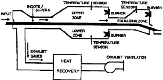
In a summary from control point of view (also see Figures I and II), these thermal processes can be operationally characterised as follows (Dimirovski

Fig. I. Input-output signal flow paths indicating the main input-output characteristics of thermal processes in high-power, multi-zone, gas/oil fired industrial furnaces.

IFAC DECOM-TT 2004

Automatic Systems for Building the Infrastructure in Developing Countries October 3 - 5, 2004 Bansko, Bulgaria

and co-authors, 2001): operating regimes of different-load as well as start-up and shut-dawn; convex input-output (control or steady-state) characteristics at the operating points; multivariable process dynamics; slow and non-linear overall dynamics, linearizable locally; varying time-delays; problematic sensor distribution; delicate sensor-actuator collocation. Provided the pressure in the furnace and the release of burned gases are operationally stabilized, the main controlled variables are the temperatures and controlling variables are the fuel/gas (energy) and air (oxygen) supply (e.g., see Dimirovski, 2000; Lu and Williams, 1983; Rihne and Tucker, 1991; Stankovski and co-authors, 1999; Yang and Lu, 1986).

Pusher furnaces in steel mills have been observed to represent rather well all operational difficulties and features of high-power industrial furnaces (Rihne and Tucker, 1991). Real-world pusher furnaces have multi-zone construction (Figure II) and indeed high installed powers. Furthermore, they are operated in difficult field environment that requires considerable maintenance support. Main disturbances come along with the heated steel mass flow and pace of the transportation line as well as the flows of hot gases and air inside the reheat processing space, albeit varying dimensions and grades of slabs in lower-grade steel processing (as Skopje Steelworks is aimed at) also act as disturbances. From industrial practice of slab pusher furnaces, it is well-known that the temperature regulatory level is capable to maintain the process variables close enough to the command set-points provided separate executive controls stabilize the pressure and maintain the general operating conditions; then the burners are properly actuated. The operational pace is imposed by the production scheduling of the slab rolling plant that follows the reheat furnace within the manufacturing line (e.g., see Yang and Lu, 1988; Dimirovski 2000; Dimirovski and co-authors, 2001).

Fig. II. The construction schematic of the three-zone 25/28 MW RZS pusher furnace at Skopje Steelworks (Dimirovski, 2000).

This paper presents the theoretical derivation (Dimirovski and Zhao, 2003) of a systems re-engineering design technique for high-power mult i-zone industrial furnaces by employing the system architecture of two-level integrated supervision and control systems , and by using theories of generalized predictive control and static optimization. The main design criterion adopted in this system

re-engineering is the improvement operational capacity of such high-power large industrial furnaces for energy savings. Recently it has been applied to systems re-engineering design of Skopje Steelworks furnace RZS 25/28 MW (see Figure II), and a great deal of the application practicalities have been published recently in a companion paper (Icev and co-authors , 2004).

The below presented systems engineering technique is believed to demonstrate well the essentiality of Professor H. H. Rosenbrock’s remarkable statement (1977, p. 390): "My own conclusion is that engineering is an art rather than a science, and by saying this I imply a higher, not a lower status". The rest of this paper is written as follows. In the next Section 2, an overview discussion on problem analysis and the background research is given. The subsequent Section 3 gives a presentation of the methodological approach and solving techniques applied. Then in Section 4 some sample results from the application to RZS furnace example are discussed. Conclusions and references are given thereafter.

2. ANALYSIS OF THE PROBLEM AND BACKGROUND RESEARCH

The overall control task is to drive the process to the desired thermodynamic equilibrium and to regulate it there as well as to maintain the temperature profile through the plant. However the economic reasons, in particular the one on energy cost (fuel consumption) per product unit, and operational technical restrictions make it necessary to optimise plant operations one way or another. Due to the need of both set-point and optimization control tasks, practice and research insofar have demonstrated that there are three solving alternatives: (i) an optimally designed controller to replace the regulatory level in performing both tasks (e.g., see Lu and Williams, 1983); (ii) an optimization expert system is combined with executive regulatory controls to perform both tasks (e.g. see Yang and Lu, 1988); (iii) a supervisory set-point optimization control is superimposed while retaining the classical regulatory level (e.g., see Marlin, 2000; Ogata, 2002) for the role of executive controls .

Industrial practice and the background research have demonstrated that the first alternative hardly leads to feasible implementation designs and that the second one requires a costly development of an appropriate expert system, employing both heuristics and mathematical modelling. It has been found in the course of research investigations carried out recently (e.g. Dimirovski and co-authors, 2001; Dimirovski and Zhao, 2003; Icev and co-authors , 2004) that the third design alternative is worth exploring for practical cost-effectiveness and maintenance reasons. In turn, this research has led to a novel system (re -) engineering design technique, to the presentation of which this invited paper is devoted.

2.1. General Conceptualization of the Problem

The systems (re-)engineering design by employing combined control and optimization methods is by itself a compromising quest to meet some main objective criteria while satisfying unavoidable engineering constraints and requirements (Lu, 1992). From the viewpoint of computer process control (Lu and Williams, 1983; Yang and Lu, 1986, 1988, the investigated problem of integrated supervisory-plus-regulatory control for industrial multi-zone pusher-type furnaces as an optimization system re-engineering problem may be formulated (Dimirovski and Zhao, 2003) in general conceptualizing terms as outlined below.

Let us assume there is available some model, providing either real-time estimation or predication of the internal process information, to be used as a resource for supervisory optimization control. Then it becomes possible to select a vector of admissible controls , say

U

(

k

)





u

1

(

k

)

.

.

.

u

_r

(

k

)



T, within some time horizon

T

_H, such that some performance index



  



1 0

))

(

),

(

(

H T k k

k

Y

k

U

unction

ObjectiveF

J

(1) is minimised subject to

)

),

(

),

(

(

)

1

(

k

f

Y

k

U

k

P

Y





,

Y

(

0

)



Y

₀, (2) Y

SP

Y



,

U



SP

_U,

P





_P. (3) In here,

U

represents a control vector for process optimization, which could define the reference set-points to local lower control level,

Y

represents a vector of feasible controlled variables, and

P

represents a vector of real-valued parameters and possibly some quantitative and/or qualitative constraints within some pre -specified domain.

The formulated optimization problem can be solved via either of approaches: directly (linear case with a quadratic criterion) or indirectly (non-linear case with Kuhn-Tucker conditions) through numerical computations (e.g. see Luenberger, 1984); or by an iterative heuristic search (e.g. see Lu, 1992); or by math-analytical nonlinear optimal control synthesis (e.g. see Zhao, 1993).

2.2. A Survey of the Relevant Background Research

In the literature, there may be found many studies that deal with set-point optimisation based on steady-state and/or dynamic models. Hence, this survey is by no means exhaustive, and the interested reader should consult the literature cited in the selected references for this paper.

Becerra and co-authors (1999), departing from steady-state model, have proposed a multi-objective predictive formulation that includes both economic

and regulatory objectives. There the regulatory level comprises a constrained non-linear controller the set-points of which are computed by the optimisation level whereby the parameters of the steady-state models are adapted on-line. Zheng and co-authors (1999) have reported a hierarchical control strategy in order to maximise the profit of a chemical plant. They used the steady-state process models to determine the set-points so that an economic objective function is optimised. Munoz and Cipriano (1999) have elaborated an economic control strategy for a mineral processing plant. Their strategy uses a regulatory level based on multi-variable predictive controllers and a global economic optimiser in order to determine the set-points of the predictive controllers. They have considered non-linear steady-state models of the grinding process and dynamic models of the flotation process given the pragmatic observation that time constants of the flotation are smaller than the ones of the grinding processes as a well-posed engineering reason.

De Prada and Va lentin (1996) have proposed a design approach that is rather appealing for case-studies of industrial furnaces. In order to determine optimized level set-points for the regulatory of a sugar processing plant, they have proposed a predictive control strategy based on an economic index optimisation. They obtained the optimal set-points at the supervisory level by optimising a multi-variable objective function. And the regulatory level is solved by using the GPC algorithm while also including constraints on the amplitude and on the slew rate of executive (manipulated) variables and the limits on controlled variables. The same predictors and constraints as for the regulatory level GPC controllers are used to solve the optimisation problem. The optimisation variables correspond to the increments of the executive variables. The optimal set-points are defined as the values of the controlled variables at time instant

t



N

_y, which corresponds to the optimal increments of the obtained executive variables. This procedure is repeated for each sampling instant, thus resulting in dynamically optimal set-points.

Indeed, model-based predictive control algorithms have been successfully applied to many different industrial processes, since the operational and economical criteria may be incorporated using an objective function to calculate the control action (e.g., see Richalet and co-authors, 1978; Richalet, 1992; Clarke and co-authors 1987, 1992, 1994; Garcia and co-authors, 1989). Moreover, in their very essence, these control strategies rely on the optimisation of the future process behaviour with respect to the future values of the executive control (process manipulated variables) and their extension to use non-linear process models is motivated by improved quality of the prediction of inputs and outputs (Allgower and co-authors, 1999). This way, non-linear predictive controls are derived albeit these do not have a specific control strategy of their own but rather utilise the methods associated with linear

predictive control via optimisation of an objective function, with constraints possibly (Ansari and Tade, 2000).

Tsang and Clarke (1988) have derived a GPC algorithm in which the constraints on executive control variables for two sampling instants of the control horizon were also incorporated. Subsequently, Demircioglu and Clarke (1992) have presented a continuous time GPC controller design based on state space models with constraints in which system stability was also ensured. A similar problem was solved by Camacho (1993) where constraints on both executive control and controlled variables were incorporated. In this case, to reduce the computing effort, the solution was obtained by transforming the quadratic optimisation problem into a linear optimisation problem. Along these lines, Camaco and Burdons (1998) have presented as a benchmark a simple furnace heat transfer and the respective GPC designs, which is of direct importance for the case of industrial furnaces as the one in our case study (Icev and co-authors, 2004). The guiding idea in this research was to improve furnace operation so that some more ‘calm’ regulatory controls are obtained via slightly time-varying set-points to the regulatory level, which in turn are obtained by using general predictive control concepts and constrained optimization. Another objective is to employ rather simple and math-analytical models that lead to a feasible two-level control strategy. An appropriate objective function is to be minimized for this purpose similarly as in works by Camaco (1993), De Prada and Valentin (1996), Munoz and Cipriano (1999). This objective function may represent several relevant parameters such as operational costs, control energy consumption and even other criteria, including also regulatory objectives of integrated square of the tracking error. Hence, it was adopted in this study.

3. SOLUTION DERIVATION FOR THE SUPERVISORY PREDICTIVE CONTROL BASED

DESIGN

The adopted solving approach to the problem of concern is as follows: firstly, a good design of the regulatory level that will provide executive controls (vector

u

) to the supervisory level for controlling measured process variables (vector

y

) while compensating the non-measured varying disturbances (vector

e

); and secondly, an optimized design (via minimizing a suitable performance objective function

J

) of the supervisory level to determine the optimal set-points (vector

r

) so that the relevant constraints accounted for into the performance index are satisfied (see Figure III). In principle, should it be available, an external reference trajectory (vector

w

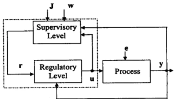
; not needed in our case study) can be included into the performance index. Hence, the supervisory level dynamically

optimises a general objective function subject to equality and inequality constraints, the overall control strategy is a hybrid one and the overall system will be stable with the conditions in (Zhao, 2001) satisfied. It should be noted, from the viewpoint of the overall system engineering, the resulting optimum may not be global but rather a local one because the regulatory level confines systems transients locally. Yet this solving approach resolves the posed problem.

Fig. III. Standard overall architecture of a two-level supervisory-plus-regulatory control system.

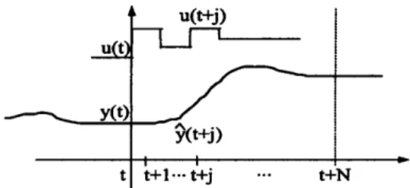
The above problem is well posed and can be solved by numerical algorithms when constraints are accounted for and/or non-linear models are used, following the third conceptual alternative (Section 1) and hints drawn from the theory of model based predictive control (Ansari and Tade, 2000; Camacho Bordons, 1998). As known from the literature (also see Figure IV), the main methodological steps in designing model based predictive controls are the following:

- The future outputs of controlled variables, for a determined horizon

N

_y, are predicted at each time instant

t

using some model of the process to be controlled. The output predictions

y

(

t



j

)

conceptually depend on the known values of process variables up to time instant

t

(the past history) and on the future control signals

u

(

t



j

)

which are to be calculated.

- The future control signals

u

(

t



j

)

are calculated by optimising a predefined objective function (criterion of performance index) in order to keep the process as close as possible some desired reference trajectory. To the best of our knowledge, rightly in most cases and the criterion is defined in terms of some quadratic form, e.g. a quadratic function of the errors between the predicted output signal and the predicted reference trajectory and of the control effort if controlling variables are to be optimized as well as in our case study.

- The control signal

u

(t

)

is executed on the actual process, and at the next sampling instant

t



1

the values of all the controlled variables until then and of all the executive control variables until time

t

are known.

- The concept of the receding horizon is used so that only the first control action from the assumed control horizon is applied at the present time instant and kept

until the next one. Then, both the prediction and control horizons are moved one step into the future, and the procedure is repeated at the next time instant. It should be noted that a suitable process model is crucial and it has to be adopted (developed or experimentally identified), and only then model based predictive control derived.

Fig. IV. An illustration of the main idea of the model based predictive control theory (Clarke and co-authors, 1987).

In the reality, as it is the case with Skopje Steelworks (Dimirovski, 2000), steel mill industrial processes are characterized by non-stationary stochastic disturbances. Therefore, as argued by Clarke in his works (e.g., 1987, 1988, 1992), the appropriate choice is a model of the class controlled autoregressive and moving-average process. Its general representation for single-input-single-output case and constant sampling period (the equidistant time-shifting intervals) is given as follows:







 

₎

₍

₎

₍

₎

₍

₎

₍

₎

_/

(

_q

1

_y

_t

_B

_q

1

_u

_t

_e

_t

A

(4)

with

q

1 the backward shift operator (i.e.

)

1

(

)

(

1

_

_



_v

_t

_v

_t

q

) and





1



q

1, where

e

(t

)

represents a zero mean white noise; the appropriate polynomials in

q

1 are given by

na na

q

a

q

a

q

A



_

_

1

_

_

_

_

 1 1

₎

₁

(

, (4 a ) nb nb

q

b

q

b

q

B







1











 1 1

1

)

(

. (4 b)

Thus, given a design of the regulatory control level implying fixed control algorithms, the respective model for the supervisory level may be represented by the following expression:

)

(

)

(

)

(

)

(

)

(

)

(

_q

1

_u

_t

_B

_q

1

_r

_t

_B

_q

1

_y

_t

A

_rc 



_rc 



_ry  (5) with nra nrc rc rc

q

a

q

a

q

A







1









 1 1

1

)

(

, (5 a) nrb nrc rc rc

q

b

q

b

q

B







1











 1 1

₎

₁

(

, (5 b) nry nry ry ry ry

q

b

b

q

b

q

B

(

1

)



₀



₁ 1









 . (5 c) The objective function, representing the optimization criterion at the supervisory level, has to account for accounts for the dynamical behaviour over the prediction-horizons. The class of objective functions as the ones used in (Tsang and Clarke, 1988;

Camaco, 1993; De Prada and Valentin, 1996; Camaco and Burdons, 1998; Munoz and Cipriano, 1999) is apparently well justified with respect to both controlled and control variables, and was adopted in our work too. That objective function may represent different optimisation goals at the supervisory level and the operational costs or the profit or the process energy consumption of a plant, in particular. In its scalar form, the objective function may be given as follows:





 

















y Nu i i u N j j y

y

t

j

u

t

i

J

1 2 1 2

₍

₎

_ˆ

₍

₁

₎

ˆ



 











y u N j N i ji yu

y

t

j

u

t

i

1 1

)

1

(

)

(

ˆ



 











u N i j u

u

t

i

1 2

₍

₁

₎









u N i j y

y

t

j

1

)

(

ˆ

ξ





  













u u N i i u N i i u

u

t

i

u

t

i

1 1

)

1

(

)

1

(

_ξ

ξ

. (6)

I

n it the individual quantities denote:

N

_u and

N

_y are prediction horizons;

y

(

t



j

)

are the j-step ahead predictions of the controlled variables based on data up to time

t

;

u

(

t

 i



1

)

are the executive controls (manipulated variables); and



u

(

t



i



1

)

are the increments of the executive controls;



_yj,

i u



,



_yuji,



_i_u and

ξ

_yj,

ξ

_ui,

ξ

_i_u are suitable weighting sequence matrices and vectors. (Notice, if known in advance, an external reference trajectory

)

(t

w

w



can also be included into the objective function as appropriate.)

In normal furnace operation, practical operating characteristics of actuators also impose constraints on the amplitude and the slew rate of the manipulated process variables, besides the limits imposed on the controlled process variables. Hence, the following constraints ought to be observed:

- amplitude limits on the controlled process variables,

y

N

j



1

,

...,

max min

y

ˆ

(

t

j

)

y

y







; (7) - amplitude limits on the executive control (manipulated) variables,

i



1

,

...,

N

_u

max min

u

(

t

i

1

)

u

u









; (8) - increment constraints on the executive control (manipulated) variables,

i



1

,

...,

N

_u

max min

u

(

t

i

1

)

u

u















. (9)

Notice that the constraints are imposed on

y

ˆ

(

t



j

)

, that is the

j



th

step ahead prediction of the

controlled process variables. The control action is to be obtained by minimising the objective function (6) under the equality constraints (5) and the inequality constraints (7)-(9). For this purpose, prediction of the control variables is calculated as a function of past values of the input controls and measured outputs and of a horizon future control actions.

3.1. An Outline of the Solving Methodology

As known from the literature (Luneberger, 1984), an explicit direct solution to this optimization problem can be obtained if the criterion is quadratic, the model is linear, and there are no constraints. This case is of more academic nature, because in practice there unavoidable constraints for many technological reasons, and so is the industrial furnace operation considered. Thus only a numerical optimisation indirect solution can be sought via introducing a Lagrangian function, typically, using Kuhn-Tucker conditions (Luneberger, 1984).

Further, for practical reasons with regard to computational effort involved, the optimization variables may be reduced to:

y

ˆ

(

t



1

)

, …,

)

(

ˆ

t

N

_y

y



;

u

(t

)

,

u

(

t



1

)

, …,

u

(

t



N

_u

)

,

)

(t

r

,

r

(

t



1

)

, …,

r

(

t



N

_y

)

. In turn, the constraints are slightly reduced too. In addition, on the grounds of the process model for predictive control and by recalling that the expectation of noise disturbances at time

t



j

is

E



e

(

t

 j

)





0

, the equality constraints on the controlled variable predictions for

j



1

,

...,

N

_y become:

























)

ˆ

(

1

)

ˆ

(

)

(

ˆ

t

j

a

₁

y

t

j

a

_na

y

t

j

n

_a

y

0

)

(

)

1

(

1

u

t



j













b

nb

u

t



j



n

b



b

. (10) By making using this intermediate result, constraints on the predictions of the controlled process variables as functions of the increments of the executive controls are simplified to:

             ) ( 1)ˆ( 1) ˆ( 1) ( ˆt j a₁ yt j a_nayt j n_a y

0

)

(

)

1

(

1



u

t



j











b

nb



u

t



j



n

b



b

. (11) Similarly, from the model of the regulatory control level, the equality constraints on the executive controls for,

i



1

,

...,

N

_u, are found to be as follows:             1) ( 2) ( ) (t i a_1rcu t i a_narcu t i n_arc u



















1

)

(

2

)

(

₁ 0

r

t

i

b

r

t

i

b

_{rc rc}













b

_nbrc

r

(

t

n

_brc

)

















1

)

ˆ

(

2

)

(

ˆ

₁ 0

y

t

i

b

y

t

i

b

yrc yrc

0

)

(

ˆ













b

nbyrc

y

t

n

byrc . (12)

Now, by making use of this result, the equality constraints on the increments of the executive controls, for

i



1

,

...,

N

_u, can be found be represented as follows:























u

(

t

i

1

)

a

_1rc

u

(

t

i

2

)















a

_narc

u

(

t

i

n

_arc

)





















b

_0rc

r

(

t

i

1

)

(

b

_1rc

b

_0rc

)

r

(

t

i

2

)















b

_nbrc

r

(

t

n

_brc

1

)























b

₀yrc

y

ˆ

(

t

i

1

)

(

b

₁yrc

b

₀yrc

)

y

ˆ

(

t

i

2

)

0

)

(

ˆ













b

nbyrc

y

t

n

byrc . (13)

Therefore, it is clear that the standard formulation of constrained non-linear optimization problem can be used. This problem now can be re-formulated (Luenberger, 1984) as follows:

x

x

x

F

Min

_M

r

,

...,

)

(

₁ (14) subject to

0

)

(

x



g

_i

r

,

i



1

,

...,

m

, (15)

0

)

(

x



g

j

r

,

j



m



1

,

...,

n

. (16)

Here

F

(

)

is a non-linear function to be minimized with respect to the vector

xr

of optimized variables so that the constraints are satisfied, with

g

_i

(x

r

)

representing the functions of equality and

g

j

(x

r

)

the functions of inequality constraints. In turn, Lagrangian function for this problem is:





  







n m j j j m i i i

x

g

x

g

x

F

x

L

1 1

)

(

)

(

)

(

)

,

(

r

λ

r

r

λ

r

λ

r

(17) Hence, Kuhn-Tucker are as follows:

0

)

,

(





_x

L

rx

_λ

r

, (18)

0

)

(

x



g

_i i

r

λ

,

i



1

,

...,

m

, (19)

0

)

(

x



g

j j

r

λ

,

j



m



1

,

...,

n

, (20)

0



j

λ

,

j



m



1

,

...,

n

. (21) In here



_x is the gradient operator of the scalar function

L

(



,



)

with respect to the vector

xr

. Note, the symbols

λ

_i,

λ

_j for denoting Lagrangean are the traditional ones. But in practical applications other symbols can be chosen, which was done in our case study. This will be seen in the sequel, where the above optimization relationships are applied to the considered time-discretized representation models of

the thermal process of RZS pusher furnace within control system architecture depicted in Figure III.

3.2. Solution Equations and Inequalities for the RZS Furnace

Thermal processes in industrial furnaces having finite steady states , for pragmatic reasons, stimulate the use of the well-known methods of statistic regression analysis (for input-output control characteristics) and of step-response and maximum-length PRBS-response (for process dynamics); three families of dynamic models according to the main operating power loads (e.g., 30%, 60-70%, and 90% of power load). After appropriate filtering, all these models are easily mapped into time sequences truncated at time Nt and then k-time sequence matrices, t0 < k < kNt, obtained with an appropriate sampling period Ts (note Ts = 1 min for the RZS furnace); i.e., a Toeplitz operator is derived from the sequence of MxM (NinpxNout) Markov matrices

)

(k

G

of plant process pseudo-impulse responses (Dimirovski, 2000). These models may be turned into matrices of approximate channel-transfer functions in shift operator

q

1. In turn, the necessary mathematical models for deriving the solving equations for this application example become readily available as seen in the sequel. The residing horizon for the supervisory predictive control can be determined by observing the pure time delays and the relationship between pure delay and inertial times

δ



τ

ij

/(

τ

ij



T

ij

)

and

η



τ

ij

/

T

ij

(Marlin, 2000) taking into consideration the adopted sampling period

T

_s



1

[min]; that is, by observing the integer value of

d





τ

_ij

T

_s



. Since

τ

_ij is approximately the same for the main channels of the upper and lower zones (i.e.,

ii



1 and

3

) and not equal to the one of the equalizing zone (i.e.,

3

1 and

ii



) as seen from Figure 4.5, a common average time delay

τ

_av was adopted and used throughout. In turn, it appeared that the residing horizon should have minimum

H

_r



3

and maximum

H

_r



5

sampling periods; the former can further reduce the computational effort, but the latter can contribute to the quality of supervisory control design.

The resulting controlled autoregressive and moving-average models with regard to

d





τ

_ii

T

_s



, have the form:







 

/

)

(

)

(

)

(

)

(

)

(

_q

1

_y

_t

_B

_q

1

_u

_t

_e

_t

A

_{ii i ii i ij} (22) with 1 1

₎

₁

_exp(

_/

₎

(

_q



_

_

_

_T

_q



A

_{ii s}

_τ

_av , (23 a) ) 1 ( 1

))

/

exp(

1

(

)

(

d av s ii ii

q

K

T

q

B









τ

  . (23b )

Since the regulatory level consists of PI controllers “

K

_Pii



K

_Iii

/

s

” (which are acting on error signals “

r

_ii

(

s

)



y

_ii

(

s

)



r

_i

(

s

)



y

_i

(

s

)

” with

K

_Pii and

Iii

K

designs to produce controls “

u

_ii

(

s

)



u

_i

(

s

)

”; elaborated in the regulatory control level) Eqs. (22) become:

)

(

)

(

)

(

)

(

)

(

)

(

q

1

u

t

B

q

1

r

t

B

q

1

y

t

A

_rci  _i



_rci  _i



_ryi  (24) with 1 1

₎

₁

(

_q



_

_

_q



A

i rc , (24 a)

,

)

5

.

0

(

)

5

.

0

(

)

(

1 1  











q

K

K

T

K

K

T

q

B

Pii ii s Pii ii s i rc (24b)

.

)

5

.

0

(

)

5

.

0

(

)

(

1 1  













q

K

K

T

K

K

T

q

B

Pii ii s Pii ii s i ry (24 c)

Given the engineering construction of the furnace (robust construction of batteries of burners and actuators at each zone) and the operating point with

midrange

U

, the inequality constraints on magnitude variations of the executive control variables were adopted. These constitute



20

%

of the maximum battery flow rate (see Eq. (8)), for ahead time steps

4

...,

,

1



i

), and these constrains along with actuator robustness allowed for neglecting the constraints on control increments (see Eq. (9)). With these magnitude constraints on controls and the constant pusher pace (also, see Figure V), the thermodynamic reasons ensure that the variations of controlled temperatures will remain close to the desired operating points, i.e. the initial condition

)

0

(

i

y

=1150 oC within the reheat processing 1050-1250 oC (to which the furnace was driven by the start-up operation) should some disturbance has caused a departure form there (also, see Figures VI and VII).

For each channel, the energy based quadratic objective function, in its simplest form with the weighting coefficients being omitted, to be minimized is as follows:

)

3

(

ˆ

)

2

(

ˆ

)

1

(

ˆ

2

_

_

2

_

_

2

_



y

t

y

t

y

t

J

i

)

3

(

)

2

(

)

1

(

)

(

2 2 2 2

_

_

_

_

_

_



u

t

u

t

u

t

u

t

.(25)

The equality constraints associated with the controlled temperatures, which are derived from Eq. (10), result in the following equations:



 )

(

t

j

y

_i

exp(



T

_s

/

_τ

_av

)

y

(

t



j



1

)



0

)

3

(

))

/

exp(

1

(













K

_ii

T

_s

_τ

_av

u

t

j

,

3

...,

,

1



j

. (26) Of course, some weighting coefficients can be introduced in (25) for the sake of further design freedom. Needless to say, this was not found useful.

The equality constraints associated with the executive controls (or manipulated process variables) - the fuel flow rates, which are derived from Eq. (12), lead to the following set of equations:













1

)

(

2

)

(

t

i

u

t

i

u











(

0

.

5

T

_s

K

_ii

K

_Pii

)

_δ

r

(

t

i

1

)











(

0

.

5

T

_s

K

_ii

K

_Pii

)

_δ

r

(

t

i

2

)











(

0

.

5

T

_s

K

_ii

K

_Pii

)

y

(

t

i

1

)

0

)

2

(

)

5

.

0

(











T

_s

K

_ii

K

_Pii

y

t

i

,

3

...,

,

1



j

. (27) The sets of Kuhn-Tucker conditions for the objective function, with regard to Eq. (4. 9) and the inequality and the equality constraints Eqs. (26)-(27), after a rather lengthy derivation finally become:







j

j

t

y

(

)

λ

2

exp(



T

s

/

τ

av

)

λ

j_1









(

0

.

5

T

s

K

ii

K

Pii

)

μ

j_1

0

)

5

.

0

(



2





T

s

K

ii

K

Pii

μ

j_ ,

j



1

,

2

; (28) 3

)

3

(

2

y

t





_λ



(

0

.

5

T

_s

K

_ii



K

_Pii

)

_μ

₄



0

,

2

,

1



j

; (29) 2 1

)

(

2

u

t



_{μ }

_μ



K

ii

(

1



exp(



T

s

/

τ

av

))

λ

₃



0

min 1





_ν

u _,

_j

_

₁

_,

₂

_{; (30)}

0

)

(

2

min 2 1











_{ } u i i i

i

t

u

_μ

_μ

_ν

,

j



1

,

2

; (31) 2 1

)

(

2

u

t



_{μ }

_μ



K

ii

(

1



exp(



T

s

/

τ

av

))

λ

₃



0

max 1





_ν

u _,

_j

_

₁

_,

₂

_{; (32)}

0

)

(

2

max 2 1











_{ } u i i i

i

t

u

_μ

_μ

_ν

,

j



1

,

2

; (33)

0

)

3

(

2

u

t





_μ

₄



;

j



1

,

2

; (34)

0

)

5

.

0

(



₁





T

s

K

ii

K

Pii

μ

;

j



1

,

2

; (35)







(

0

.

5

T

s

K

ii

K

Pii

)

μ

j_1

0

)

5

.

0

(



2





T

s

K

ii

K

Pii

μ

j_ ,

j



1

,

2

; (36)

0

)

5

.

0

(



₄





T

_s

K

_ii

K

_Pii

_μ

,

j



1

,

2

; (37)



 )

(

(

y

t

j

exp(



T

_s

/

_τ

_av

)

y

(

t



j



1

)



))

3

(

))

/

exp(

1

(











K

_ii

T

_s

_τ

_av

u

t

j

λ

j



0

,

3

...,

,

1



j

; (38)













1

)

(

2

)

(

(

u

t

i

u

t

i











(

0

.

5

T

_s

K

_ii

K

_Pii

)

_δ

r

(

t

i

1

)











(

0

.

5

T

_s

K

_ii

K

_Pii

)

_δ

r

(

t

i

2

)











(

0

.

5

T

_s

K

_ii

K

_Pii

)

y

(

t

i

1

)

i Pii ii s

K

K

y

t

i

T

)

(

2

))

μ

5

.

0

(











0

,

4

,...,

1



i

; (39)

0

)

1

(





min





u i

i

t

u

ν

,

i



1

,...,

4

; (40)

0

)

1

(





max





u i

i

t

u

_ν

,

i



1

,...,

4

; (41) and

0

min



u i

ν

, umax



0

i

ν

,

i



1

,...,

4

. (42) The optimal solutions for the executive control signals of the supervisory predictive controller,

)

(t

r

δ

, can be obtained by taking

λ

₁



0

,

λ

₂



0

,

0

3



λ

, and

μ

₁



0

, …,

μ

₄



0

. When the constraints are active as considered above and no further changing of executive controls is allowed for, via the non-linear programming method (Luenberger, 1984) for Eqs. (26)-(42), the time -varying set-points are determined as follows:











(

1

/(

0

.

5

))(

(

1

)

)

(

t

T

K

K

u

t

r

NLin _{s ii Pii} i

δ













(

0

.

5

T

_s

K

_ii

K

_Pii

)(

r

(

t

1

)

y

(

t

1

))

))

(

)

5

.

0

(

T

_s

K

_ii



K

_Pii

y

t

, (43) where the index

i



1

,...,

3

now indicates the channel of the regulatory control level (i.e.,

ii

=1, 2, 3). When the inequality constraints are not active (Langranean multipliers are not needed, hence non-existent) and further changing of executive controls is allowed for, the above optimization problem becomes a linear one and is solved via the linear programming method (Luenberger, 1984). The time-varying set-points are found as follows:











(

1

/(

0

.

5

))(

(

1

)

)

(

t

T

K

K

u

t

r

s ii Pii Lin i

δ













(

0

.

5

T

_s

K

_ii

K

_Pii

)(

r

(

t

1

)

y

(

t

1

))







(

0

.

5

T

_s

K

_ii

K

_Pii

)

y

(

t

))























)

(

)

/

(

(exp

))

/

(

exp

1

(

1

)(

5

.

0

(

)

/

exp(

1

(

3 2 2

t

y

T

T

K

K

K

T

T

K

av s av s ii Pii ii s av s ii

τ

τ

τ











exp

2

(

_T

/

)(

0

.

5

_T

_K

_K

)

_u

(

_t

2

)

Pii ii s av s

τ

))

1

(

)

5

.

0

)(

/

exp(









T

_s

τ

_av

T

_s

K

_ii

K

_Pii

u

t

,(44) where the index

i



1

,...,

3

again indicates the channel of the regulatory control level.

Equations (43) and (44) have been derived for computing the prediction-guided reference set-points for optimized operation of the particular case of RZS furnace. It should be noted, however, given the physical nature of thermal processes in industrial furnaces and their multi-zone construction, equations involving similar process parameters can be derived following the same methodology.

4. SOME RESULTS FOR RZS PUSHER FURNACE AND DISCUSSION

In here, only sample results for the case-study of RZS furnace (see Figure II) at Skopje Steelworks – three zones; total size 25x12x8 m; maximum installed 28MW and operating power 25 MW – are given and discussed from the overall systems engineering point of view. Thermal process in this 3-zone furnace, with respect to the actuator-sensor collocation, is a 3x3 (Ninp x Nout) multivariable process with a considerable pure time delay phenomenon both for the regulatory and the supervisory control level. Therefore simplified low-order models were utilised for designing executive furnace controls of the regulatory level such as represented by Eq. (45) below.

Fig. V. Operating steady-state characteristics with respect to operating pace: Slab temperatures Tt, Tc, Tb as functions of pusher pace; upper curve at slab top surface Tt, lower curve Tb - bottom surface; middle curve Tc – slab centre. The RZS furnace is primarily aimed at thermal treatment of low-grade steel slabs, before they enter the hot-rolling mill. When necessary, however, steel ingots are also processed for reasons of sustained run of the business, thus making its operation more delicate. Hence, the economic issue of energy saving is rather important.

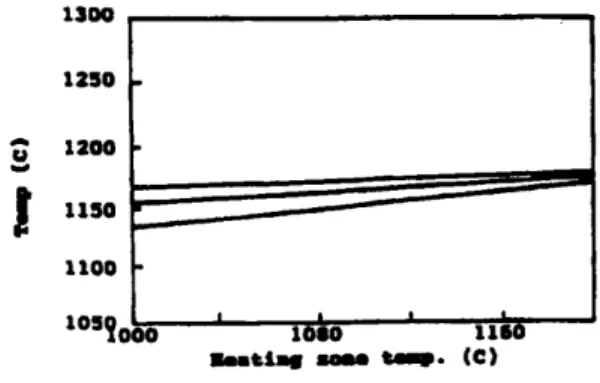
Typical steel reheat processing takes place at the processing temperatures 900-1100 oC / 1050-1250 oC / 1200-1400 oC. Hence a process identification study was prerequisite in order to obtain families of steady-state (e.g., characteristics in Figure VI) and dynamic process models (e.g., pseudo-impulse responses and difference equations; see Figure VII) from the control point of view. The furnace is operated in a steady-state regime at a given pusher pace depending on slab/ingot size and other metallurgical specifications (these are beyond our expertise and not of concern in here) as shown by the respective characteristic curves in Figure V (the standard 1050-1250 oC processing). For the operating regime 1050-1250 oC, the respective characteristic curves of the heating furnace zones (lower and upper) for the slab temperatures are shown in Figure VI. It should be noted, the post-design observation showed that diagram may not be entirely precise; most likely the actual curves are not that close to the linear ones.

The regulatory design alone (also see Figure IX) remains within the framework of the traditional implementation of a human-operator supervised classical scheme of overall adjusted and locally fine tuned SISO controls. Subsequently, certain additional improvements have been made following appropriate engineering investigations. With the goal to exclude or reduce the role of human operator (except for the start-up/shut-dawn regimes), the research reported in here is along the same lines and an enhanced real-time process control ensuring about 4% cost saving for fuels has been achieved for furnace operations according to characteristics in Figures V-VI (Icev and co-authors, 2004).

Fig. VI. Operating steady-state characteristics of heating zones : Slab temperatures Tt, Tc, Tb as functions of furnace heating zone temperature for the standard processing regime 1050-1250 o_{C (after overall control system redesign).}

Characteristics curves for Tt and Tb in Figures V-VI have been obtained off real time using special measurement technology, whereas the one for Tc is estimated by some combined empirical experimentation and analysis, or by a special Kalman filter, or by means of a special heat transfer simulation model. The main goal of the overall control system is to ensure achieving such a characteristic curve Tc for the inside temperatures of the slab, which guarantees its quality mechanical processing in the associated hot-rolling mill. Further, it should be noted that slabs are heated mainly due to radiation transfer from hot furnace walls, and convection heat transfer due to forced counter-flow of hot gases is minor (see Figure II). Besides the tracks, on which slabs are sliding when pushed, cause slightly lower heated skid-marks at the bottom of slabs. For these reasons, it is important to achieve heating zone operating characteristics as close as possible to the ones in Figure VI because are controls executive based on measured wall temperatures. Finally, for the constructive zones of the furnace, it is pointed out that any furnace control system design operates on the grounds of on on-line measurements of temperatures furnace walls and not of slabs, when implemented. That is, in this case study, these are the wall temperatures of the lower and upper heating zones and the equalizing (or soaking) zone as shown in Figure II.

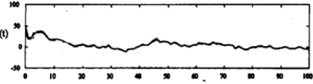
Fig. VII. A sample case of step-response tests at operating steady-state temperature 1150 oC; time in [min] and temperature gradation in tens of [o_C].

For the furnace identification (Ljung, 1999) under operating conditions, the input signals had be confined in ranges from (0.03-0.05) to (0.10-0.15) of the maximum magnitude of executive control inputs. Following a choice of 5-10% of the maximum input signal (fuel flow) allowed % of valve opening and the records of a number of step responses for every input, a family of resulting traditional first-order-lag (Ziegler-Nichols) and dead-time-second-order lag (Küpfmüller-Strejc) with ranges of values, respectively, via known theory (Marlin, 2000; Ogata, 2002) have been identified.

Process dynamics is a typical one (see Figure VI I) and non-periodic, which may be approximated by a ‘pure’ time-delay and ‘inertial’ time -lag. Combining these results with model PRBS-response identification and relevant data processing (MATLAB-Systems Identification Toolbox) it was possible to obtain sets of fairly good time -delay first and second order models, the latter represented by

)

1

)(

1

/(

)

exp(

)

(

s



K



s

T

1



T

2

s



G

ij ij

τ

ij (45)

where matrix of process gains is given by K = /Q. Thereafter the respective discrete-time representations in shift-operator

q

1, presented in the previous s ection, were readily derived.

Besides, on the grounds of a series of step-response identification it was possible to identify value ranges for the main attributes of slab heating process dynamics: steady-state (SS) gains

K

_ij (in [oC/MJ/min]) and pure time -delays (dead-times)

τ

_ij (in [min]) within each of the process transfer paths. Regarding the main process channels (transducer-actuator paths of the equalizing, lower, and upper zones) the values of SS gains range within 7.25-8. 95, 4.10-6.50, and 1.50-1.70, while time -delays (see Figure VIII) within 1.50-1.70, 2.10-3.90, and 3.90-7.20, respectively, depending on the actual power load, e.g. of 30%, 60-70%, and 90%. Note that these variations account for operating process uncertainties to some extent.

Fig. VIII. Estimates of operational time delay variations in the three furnace zones due to load variations and other disturbances (based on step responses); value ranges within the text. At this point, it is emphasised that a quality design of the regulatory control level is prerequisite for applying the optimizing supervision and control strategy presented in Section 3. A careful design study of the regulatory control level should be carried for each particular industrial furnace, so as to achieve high-quality performance in the presence of changing loads, hence varying time -delays and disturbances.

Closed-loop step performance at 90% load

Closed -loop step performance at 60% load

Closed -loop step performance at 30% load

Fig. IX. Performance of the closed-loop control of the designed regulatory level: Fairly simple SS- decoupling-plus-PI regulatory control amenable for easy maintenance and tuning (noise filtered).