© TÜBİTAK
doi:10.3906/fiz-2004-7 h t t p : / / j o u r n a l s . t u b i t a k . g o v . t r / p h y s i c s /
Research Article
Network dynamics reconstruction from data
Deniz EROĞLU∗
Department of Bioinformatics and Genetics, Faculty of Engineering and Natural Sciences, Kadir Has University, İstanbul, Turkey
Received: 09.04.2020 • Accepted/Published Online: 09.08.2020 • Final Version: 31.08.2020
Abstract: We consider the problem of recovering the model of a complex network of interacting dynamical units from
time series of observations. We focus on typical networks which exhibit heterogeneous degrees, i.e. where the number of connections varies widely across the network, and the coupling strength for a single interaction is small. In these networks, the behavior of each unit varies according to their connectivity. Under these mild assumptions, our method provides an effective network reconstruction of the network dynamics. The method is robust to a certain size of noise and only requires relatively short time series on the state variable of most nodes to determine: how well-connected a particular node is, the distribution of the nodes’ degrees in the network, and the underlying dynamics.
Key words: Dynamical systems, complex networks
1. Introduction
Many severe disorders such as Parkinson’s disease, schizophrenia, and dyslexia are believed to be associated with anomalous brain connectivity [1]. The key role that connectivity plays in a network function is not restricted to neuroscience. Indeed, examples are found in engineering [2,3], physics [4,5], and biology [6–8]. To understand and control such systems, as well as to predict sudden changes of behavior, one often needs a faithful description of the governing rules and connectivity structure of the networks involved.
Reconstructing the connectivity structure of a network from data is a daunting task due to the high dimensionality of the network dynamics. Often there is no lack of data for the observed dynamics at each node, and the main challenge is to understand how to use this data to understand how the dynamics is influenced by the thousands or millions of interactions among the elements of the network [9,10].
Recently, the problem of reconstructing the network connectivity from multivariate data has attracted a great deal of attention [11–16]. Advanced methods can tackle the case of a few coupled phase oscillators [17–23]. For networks of moderate size, approaches based on information measures can be used under the assumption that the interaction strength is large enough to induce nonlinear collective dynamics [24–26]. However, in large networks the interaction strength per connection is typically weak and the multitude of interactions are organized in an intricate maze composed of communities having highly connected nodes coexisting with poorly connected ones [27]. In such situations, the weak interaction allied with the chaotic dynamics of the nodes leads to an observed dynamics that, at first sight, looks like a noise signal, thereby offering a great challenge to reconstruction methods.
In this article, we provide a method to recover the statistical properties of the connectivity when the connection strength per link is weak. Our approach works when the network structure exhibits disparate
∗Correspondence: [email protected]
connectivity scales such as scale-free (SF) degree distribution and when the isolated dynamics of the nodes is chaotic. With relatively short time series, our method can recover the degree distribution, build a model for the isolated dynamics and the coupling function. We also illustrate the power of this method against a certain size of additive noise from a single multivariate time series.
2. Model: network dynamics
We consider a network of N nodes with nonidentical nonlinear isolated dynamics and pairwise interaction. Such network can be described by its adjacency matrix A, whose entry Aij equals 1 if nodes i and j are connected
and 0 otherwise. The time evolution of the dynamics on the network is determined by
xi(t + 1) = fi(xi(t)) + α N
∑
j=1
Aijh(xi(t), xj(t)). (1)
When performing reconstruction from data, however, the isolated local dynamics fi: M → M , the
coupling function h, the coupling parameter α , the adjacency matrix A and even the dimension of the space M are unknown. This class of equations describe the dynamics of many important complex systems found in neuroscience [28], engineering [2,3], superconductors [5], and biology [8] among others.
Our two basic assumptions are (i) local dynamics is close to some unknown ergodic and chaotic map f , i.e. ∥f −fi∥ ≤ δ (this is usual in applications [29,30]) and (ii) the connectivity of the network is heterogeneous.
This means that the number of interactions ‘received’ by a node i (given by its in-degree ki=
∑
jAij), varies
widely across the network. More precisely, ki is very small compared to N for most i , but for a relatively small
number of nodes, called hubs, ki is much larger (e.g. a SF network). Our method tests whether these two basic
assumptions (i) and (ii) hold and from then on performs the reconstruction of the model.
We assume that we have access to a time series of observations yi(t) = ϕ(xi(t)) at each node, where ϕ is
a projection to a state variable. This is often the case in applications. For instance, in neurons we have access to a membrane potential and in electronic circuits to the voltages. From this single variable, we will reconstruct the model.
3. Functional networks
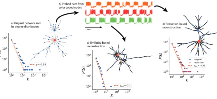
Suppose that a multivariate time series is given for some fixed, but unknown, network and dynamical parameters Figures 1a and 1b. A fundamental question is whether one can recover the interaction structure from these measurements. The relation between time series and network structure is not unique, but it is believed that the important statistical information about the network connectivity is manifested in the time series [31–33].
To access the network connectivity, it is common to introduce a functional network. This consists in assigning a numerical value to the similarity between the time series of any two nodes and then construct a network according to the values obtained. There are many ways to assign a similarity value to two time series. For examples one can use correlations, mutual information, and various extensions of these [34, 35]. Let us focus on the correlation measure.
3.1. Pairwise correlations between nodes
As a measure of similarity, we use Pearson correlation between the time series yi(t) and yj(t) , t = 0, . . . , T
by the nodes i and j . Then, the intensity Si =
∑
jsij approximates how many nodes have similar behavior
to the node i . The paradigm is that studying the statistical properties of quantities such as the distribution of intensities we gain some insight into the network connectivity structure. Let us put this paradigm to the test by performing simulations on SF networks of chaotic systems.
3.2. Scale-free networks of coupled chaotic systems
We generate a power law graph of N = 104 nodes, using the model of networks with given expected degrees
[36] with local and fully chaotic dynamics given by the logistic map f (x) = 4x(1− x), coupling function h akin to diffusion h(x, y) = sin 2πy− sin 2πx. We simulate the network for a time T = 2000 to obtain the time series. We then compute the intensity Si for every node and compare its distribution with the degree distribution of
the network (see Fig 1(c)). The true structural exponent for the power law is γ = 2.53 , on the other hand, the structural exponent estimated through the functional network is γest= 3.1 yielding nearly 25% imprecision.
The functional network therefore overestimates γ . This has drastic consequences on the predicted character of the network. Indeed, the number of connections of a hub is heavily concentrated at kmax = kminN1/(γ−1). So, the relative inaccuracy in the maximal degree is N1/γ−1/γest, which, in this case, leads
to roughly 500% inaccuracy. This, in turn, has drastic consequences on the ability to predict emergence of collective behavior for the network dynamics [10,37].
Aside from inaccurate γ estimation, another striking observation in Figures1a and1c is the absence of many points at the lowest level of P (S). Abundance of low-degree nodes and rareness of high-degree nodes are common property of SF networks. The degree of such high-degree nodes are usually unique in the SF networks, therefore there are many points at the lowest level of the degree distribution. However, the correlation-based analysis is not sensitive enough to distinguish these high-degree nodes from each other. This causes the missing points on P (S) and a large deviation from the degree distribution. For these reasons, we propose a new technique to extract the structural exponent by exploring the approximate ergodic behavior of the overall network dynamics.
4. Effective networks
Our method consists in building an effective network model to describe the observations. The effective network provides a model for the local dynamics, the coupling function and the statistical properties of the network, more precisely, it recovers the degree distribution. Thus, we can build a network having statistically the same characteristics as the network that generated the data, which, along with the recovered model for the local dynamics and coupling function. Our method consists of three main steps:
Step 1 : Reduced dynamics. For the sake of clarity, we describe the procedure when the reduced
dynamics is a 1-dimensional map. Eq.1can be reduced in the following form
xi(t + 1) = fi(x(t))− αkiv(x(t)) + αξi(t). (2)
where ki is the degree of node i and ξi is finite size fluctuations due to reduction at node i , v(x) =
∫
h(y, x)dm(y) and m is the Lebesgue measure. For a precise statement and details of the general setting see [10,38].
Given the multivariate time series {y1(t), . . . , yN(t)}, we consider each time series separately and then
probability that the dynamics is low dimensional. If the time series is high dimensional, we discard it, and otherwise, once we are in the appropriate dimension, we estimate the evolution function gi(x) = fi(x)−αkiv(x)
and we continue to the next step.
Step 2: Isolated dynamics and effective coupling function. Once we have estimated gi for each
time series, we notice that for the low-degree nodes, αkiv is negligible and the dynamics at the low-degree nodes
are close to f . We identify these nodes by analysing the distribution of Si. We use the top Ntop nodes of the
highest intensity to obtain a proxy for the isolated dynamics. We then average these rules to get ⟨g⟩ ≈ f . The choice of Ntop is not fixed and depends on the number of nodes and the fluctuation σg2=⟨(gi− ⟨g⟩)2⟩. A good
heuristic to choose Ntop is σ2g/N
1/2
top ≪ 1, as we have used here.
The effective coupling function. Since αkiv = gi− ⟨g⟩, analyzing the family {gi− ⟨g⟩}Ni=1 can yield the
shape of v up to a multiplicative constant via a nonlinear regression by imposing that gi− ⟨g⟩ and gj− ⟨g⟩ are
linearly dependent. The choice of the base function for the fitting is supervised and depends on the particular application.
Step 3. Network Structural Statistics. After selecting a v that satisfactorily approximates gi− ⟨g⟩
up to a multiplicative constant over all indices i , we estimate the parameter βi = αki using a dynamic
Bayesian inference. Because the fluctuations ξi(t) are close to Gaussian we use a Gaussian likelihood function
and a Gaussian prior for the distribution of the values of βi, and hence obtain equations for the mean and
variance. We split the data into epochs of 200 points and update the mean and variance iteratively.
4.1. Application: logistic maps on scale-free networks
To compare our method and the functional network approach, we test the same system as in the functional network approach (Figures 1a–1c). Consider M = [0, 1], x = x and fi(x) = fi(x) where
f (x) := 4x(1− x). (3)
It is known that for such parameter, the map f has an absolutely continuous invariant probability measure. As a coupling function, we consider
h(xj, xi) = sin(2πxj)− sin(2πxi) (4)
and the reduction (Eq. 2) is given by xi(t + 1) = f (xi(t))− αkiv(xi(t)), where v is defined as above. Again,
we consider the reduced model gi(x) = f (x)− βiv(x) in terms of the free parameter βi= αki. Analyzing the
distribution of βi we access the distribution of the degrees. The estimate for γ obtained applying our method
is 2.55, which has an error of just 1% (Fig. 1(d)).
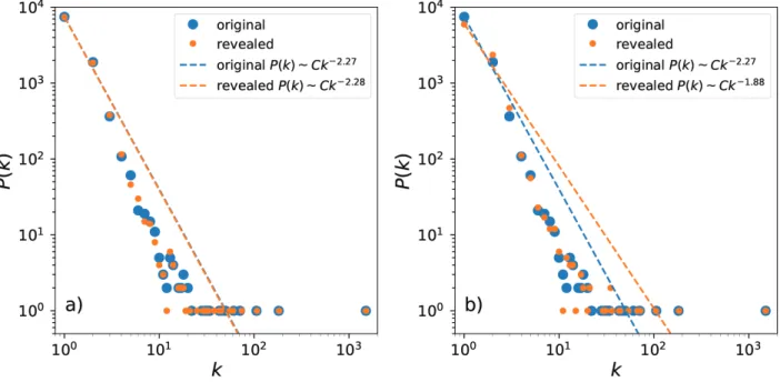
To illustrate the power of our approach, we generate SF networks with distinct values of γ , and perform our reconstruction approach to get estimates for the exponent γ . The method estimates the structural exponent with a 2% accuracy (Figure 2).
5. Robustness of the reconstruction under noise
Adding some small independent noise to the dynamics does not influence much the reconstruction procedure for the logistic map. This is a consequence of stochastic stability of the local dynamics together with the persistence of the reduction [10]. On the other hand, when the fluctuations become too large the reconstruction
Figure 1. Reconstruction of Networks Dynamics. Measuring the state of each node in time we access the performance
of the network. From time series of such measurements the goal is to reconstruct the network. Under the assumption that connections are manifested by correlations a functional network is created by measuring this quantity. Correlation analysis provides an over identification of the structural exponent. a) the original network and its degree distribution, b) the probed time series from original network, c) similarity-based reconstructed degree distribution and associated network, d) reduction-based reconstructed degree distribution and network.
Figure 2. Reconstruction of the network statistical properties for the logistic map with diffusive coupling. The degree
distribution of the network follows a power law P (k)∝ k−γ. The power law exponent γ vs the estimated one γest from
data.
will underestimate the network structure. To illustrate these effects, we consider the randomly perturbed various maps
where the random variables ηi(t) are independent over i and t , and identically distributed uniformly in the
interval [−η0, η0] . Intuitively, as long as η0< α min ki the reconstruction will go through as the noise fluctuation
will not compete with the coupling term. Notice that we normalize ∥v∥ = 1.
Now, we illustrate the robustness agains noise with three dynamical systems logistic map, Bernoulli map and Henón map. For all the applications the network structure selected as follows the system size of the network N = 105 and min ki= 1 .
5.1. Application: logistic map
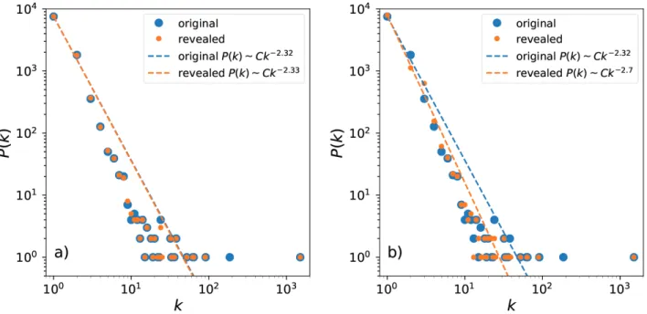
The effect of noise on coupled logistic maps for α min ki= 0.0013 is illustrated in Figure3. In inset a) the noise
has a smaller support η0 = 0.001 than the critical noise level, and the reconstruction performs accurately. In
inset b) the noise has a large support η0 = 0.003 , the reconstruction underestimate the number of low degree
nodes.
Figure 3. Performance of the reconstruction for coupled logistic maps under effect of noise. When stochastic
pertur-bations are moderate, the effective networks provide sharp estimates on the network structure. If the noise is large, the difference between the time series at low and high degree nodes becomes blurred. Inset a) shows that the reconstruction is unaffected by the noise for η0= 0.001 . b) the reconstruction of the degree distribution for η0= 0.003 cannot accurately
estimate the degree distribution.
5.2. Application: Bernoulli Map
Here, we study the effect of the noise problem on coupled Bernoulli maps. Consider M = [0, 1], x = x and
fi(x) = fi(x) where
f (x) := 2x mod 1. (5)
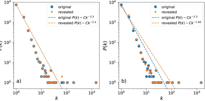
The effect of noise on coupled Bernoulli maps for α min ki= 0.002 illustrated in Figure4. In inset a) η0= 0.001 ,
the algorithm is able to reconstruct the degree distribution. In inset b) the noise has a large support η0= 0.003 ,
Figure 4. Performance of the reconstruction for coupled Bernoulli maps under effect of noise. Inset a) shows that the
reconstruction is unaffected by the noise for η0= 0.001 . b) the reconstruction of the degree distribution for η0= 0.003
cannot accurately estimate the degree distribution.
5.3. Application: Henón Map
Here, we study the effect of the noise problem on 2-dimensional coupled Henón maps,
f (x, y) = {
1− 1.4x2+ y 0.3x
with x−coupled scheme, can be represented with the following coupling matrix h,
h = [ 1 0 0 0 ] .
The effect of noise on x−coupled Henón maps for α min ki= 10−5 illustrated in Figure4. In inset a) the
noise is small η0= 10−5 and the reconstruction works well. In inset b) the noise has a large support η0= 10−4,
the reconstruction fails as in previous 1-dimensional dynamical systems applications.
6. Conclusions
We have described a general procedure that allows to reconstruct degree distribution and dynamical features from time series of observations at each node of a networked system. The method, inspired by theoretical results on the ergodic properties of coupled systems, has shown very good performances when tested on large heterogeneous networks of interacting chaotic units even when there is a small size noise is involved in the application. It exploits dynamical insights, giving estimates more accurate than those obtained with generic statistical tools only.
Figure 5. Performance of the reconstruction for x−coupled Henón maps under effect of noise. Henón map is a
2-dimensional map and the systems only coupled towards their x -components. Inset a) shows that the reconstruction is unaffected by the noise for η0= 10−5. b) the reconstruction fails for η0= 10−4 which is larger than α min ki.
Acknowledgment
We are in debt with Matteo Tanzi, Sebastian van Strien and Tiago Pereira for enlightening discussions. This work was supported by TUBITAK Grant No. 118C236.
References
[1] Bohland JW, Wu C, Barbas H, Bokil H, Bota M et al. A proposal for a coordinated effort for the determination of brainwide neuroanatomical connectivity in model organisms at a mesoscopic scale. PLoS Computational Biology 2009; 5 (3).
[2] Yadav P, McCann JA, Pereira T. Self-synchronization in duty-cycled Internet of Things (IoT) applications. IEEE Internet of Things Journal 2017; 4 (6): 2058-2069.
[3] Dörfler F, Chertkov M, Bullo F. Synchronization in complex oscillator networks and smart grids. Proceedings of the National Academy of Sciences 2013; 110 (6): 2005-2010.
[4] Komar P, Kessler EM, Bishof M, Jiang L, Sørensen AS et al. A quantum network of clocks. Nature Physics 2014; 10 (8): 582-587.
[5] Watanabe S, Strogatz SH. Constants of motion for superconducting Josephson arrays. Physica D: Nonlinear Phenomena 1994; 74 (3-4): 197-253.
[6] Néda Z, Ravasz E, Brechet Y, Vicsek T, Barabási AL. The sound of many hands clapping. Nature 2000; 403(6772): 849-850.
[7] Blasius B, Huppert A, Stone L. Complex dynamics and phase synchronization in spatially extended ecological systems. Nature 1999; 399 (6734): 354-359.
[9] Park HJ, Friston K. Structural and functional brain networks: from connections to cognition. Science 2013; 342 (6158): 1238411.
[10] Pereira T, Van Strien S, Tanzi M. Heterogeneously coupled maps: hub dynamics and emergence across connectivity layers. arXiv 2017; arXiv: 1704.06163.
[11] Gardner TS, Di Bernardo D, Lorenz D, Collins JJ. Inferring genetic networks and identifying compound mode of action via expression profiling. Science 2003; 301 (5629): 102-105.
[12] Sauer TD. Reconstruction of shared nonlinear dynamics in a network. Physical Review Letters 2004; 93 (19): 198701.
[13] Schneidman E, Berry MJ, Segev R, Bialek W. Weak pairwise correlations imply strongly correlated network states in a neural population. Nature 2006; 440 (7087): 1007-1012.
[14] Tokuda IT, Jain S, Kiss IZ, Hudson JL. Inferring phase equations from multivariate time series. Physical Review Letters 2007; 99 (6): 064101.
[15] Ren J, Wang WX, Li B, Lai YC. Noise bridges dynamical correlation and topology in coupled oscillator networks. Physical Review Letters 2010; 104 (5): 058701.
[16] Levnajić Z, Pikovsky A. Network reconstruction from random phase resetting. Physical Review Letters 2011; 107 (3): 034101.
[17] Kralemann B, Cimponeriu L, Rosenblum M, Pikovsky A, Mrowka R. Phase dynamics of coupled oscillators reconstructed from data. Physical Review E 2008; 77 (6): 066205.
[18] Penny WD, Litvak V, Fuentemilla L, Duzel E, Friston K. Dynamic causal models for phase coupling. Journal of Neuroscience Methods 2009; 183 (1): 19-30.
[19] Kralemann B, Pikovsky A, Rosenblum M. Reconstructing phase dynamics of oscillator networks. Chaos: An Interdisciplinary Journal of Nonlinear Science 2011; 21 (2): 025104.
[20] Kralemann B, Frühwirth M, Pikovsky A, Rosenblum M, Kenner T et al. In vivo cardiac phase response curve elucidates human respiratory heart rate variability. Nature Communications 2013; 4 (1): 1-9.
[21] Stankovski T, Duggento A, McClintock PV, Stefanovska A. Inference of time-evolving coupled dynamical systems in the presence of noise. Physical Review Letters 2012; 109 (2): 024101.
[22] Ota K, Aoyagi T. Direct extraction of phase dynamics from fluctuating rhythmic data based on a Bayesian approach. arXiv 2014; arXiv: 1405.4126.
[23] Cestnik, R, Rosenblum M. Reconstructing networks of pulse-coupled oscillators from spike trains. Physical Review E 2017; 96 (1): 012209.
[24] Wilmer A, De Lussanet M, Lappe M. Time-delayed mutual information of the phase as a measure of functional connectivity. PLoS One 2012; 7 (9).
[25] Lobier M, Siebenhühner F, Palva S, Palva JM. Phase transfer entropy: a novel phase-based measure for directed connectivity in networks coupled by oscillatory interactions. Neuroimage 2014; 85: 853-872.
[26] Casadiego J, Nitzan M, Hallerberg S, Timme M. Model-free inference of direct network interactions from nonlinear collective dynamics. Nature Communications 2017; 8 (1): 1-10.
[27] Zamora-López G, Zhou C, Kurths J. Cortical hubs form a module for multisensory integration on top of the hierarchy of cortical networks. Frontiers in Neuroinformatics 2010; 4: 1.
[28] Izhikevich EM. Dynamical systems in neuroscience. Cambridge, MA, USA: MIT Press, 2007.
[29] Pinto RD, Varona P, Volkovskii AR, Szücs A, Abarbanel HD et al. Synchronous behavior of two coupled electronic neurons. Physical Review E 2000; 62 (2): 2644.
[30] Eroglu D, Lamb JS, Pereira T. Synchronisation of chaos and its applications. Contemporary Physics 2017; 58 (3): 207-243.
[31] Bettinardi RG, Deco G, Karlaftis VM, Van Hartevelt TJ, Fernandes HM et al. How structure sculpts function: unveiling the contribution of anatomical connectivity to the brain’s spontaneous correlation structure. Chaos: An Interdisciplinary Journal of Nonlinear Science 2017; 27 (4): 047409.
[32] Eguiluz VM, Chialvo DR, Cecchi GA, Baliki M, Apkarian AV. Scale-free brain functional networks. Physical Review Letters 2005; 94 (1): 018102.
[33] Bullmore E, Sporns O. Complex brain networks: graph theoretical analysis of structural and functional systems. Nature Reviews Neuroscience 2009; 10 (3): 186-198.
[34] Zhang J, Small M. Complex network from pseudoperiodic time series: Topology versus dynamics. Physical Review Letters 2006; 96 (23): 238701.
[35] Greicius MD, Krasnow B, Reiss AL, Menon V. Functional connectivity in the resting brain: a network analysis of the default mode hypothesis. Proceedings of the National Academy of Sciences 2003; 100 (1): 253-258.
[36] Chung F, Lu L. Complex graphs and networks. Providence, RI, USA: American Mathematical Society, 2006. [37] Pereira T. Hub synchronization in scale-free networks. Physical Review E 2010; 82 (3): 036201.
[38] Eroglu D, Tanzi M, Van Strien S, Pereira T. Revealing dynamics, communities, and criticality from data. Physical Review X 2020; 10: 021047.