Methods and tools for visualization and management of SBGN process description maps

METHODS AND TOOLS FOR

VISUALIZATION AND MANAGEMENT OF

SBGN PROCESS DESCRIPTION MAPS

a thesis

submitted to the department of computer engineering

and the graduate school of engineering and science

of bilkent university

in partial fulfillment of the requirements

for the degree of

master of science

By

Mecit Sarı

I certify that I have read this thesis and that in my opinion it is fully adequate, in scope and in quality, as a thesis for the degree of Master of Science.

Assoc. Prof. Dr. U˘gur Do˘grus¨oz(Advisor)

I certify that I have read this thesis and that in my opinion it is fully adequate, in scope and in quality, as a thesis for the degree of Master of Science.

Assist. Prof. Dr. Burkay Gen¸c

I certify that I have read this thesis and that in my opinion it is fully adequate, in scope and in quality, as a thesis for the degree of Master of Science.

Assist. Prof. Dr. ¨Ozg¨ur S¸ahin

Approved for the Graduate School of Engineering and Science:

Prof. Dr. Levent Onural Director of the Graduate School

ABSTRACT

METHODS AND TOOLS FOR VISUALIZATION AND

MANAGEMENT OF SBGN PROCESS DESCRIPTION

MAPS

Mecit Sarı

M.S. in Computer Engineering

Supervisor: Assoc. Prof. Dr. U˘gur Do˘grus¨oz July, 2014

Graphs are commonly used to model relational information in many areas such as relational databases, software engineering, biological and social networks. In vi-sualization of graphs, automatic layout, interactive editing and complexity man-agement of crowded graphs are essential for effective utilization of underlying information.

Advances in graphical user interfaces have given rise and value to interactive editing and diagramming techniques in graph visualization. As the size of the information to be visualized vastly increased, it became harder to analyze such networks, making use of relational information needed to be acquired. To over-come this problem, sophisticated and domain-specific complexity management techniques should be provided.

The Systems Biology Graphical Notation (SBGN) has been developed over a number of years by biochemists and computer scientists to standardize visual representation of biochemical and cellular processes. SBGN introduces a concrete, detailed set of symbols for scientists to represent network of interactions, in a way that is not open to more than one interpretation. It also describes the manner, in which such graphical information should be interpreted.

The SBGN Process Description (PD) language shows how entities are influ-enced by processes, which are represented by several reaction types in a biological pathway. It can be used to show all the molecular interactions taking place in a network of biochemical entities, with the same entity appearing multiple times in the same diagram.

iv

We developed methods and tools to effectively visualize and manage SBGN-PD diagrams. Specifically, we introduced new algorithms for proper manage-ment of complexity of large SBGN-PD diagrams. These algorithms strive to keep SBGN-PD diagrams intact as complexity management takes places. In ad-dition, we provided software components and web-based tools that implement these methods. These tools use state-of-the-art web technologies and libraries.

Keywords: Bioinformatics, Biology, Graph Visualization, Pathways, SBGN, Com-plexity Management, Visualization Software, Web-based Software.

¨

OZET

T ¨

URKC

¸ E BAS

¸LIK

Mecit Sarı

Bilgisayar M¨uhendisli˘gi, Y¨uksek Lisans Tez Y¨oneticisi: Do¸c. Dr. U˘gur Do˘grus¨oz

Temmuz, 2014

C¸ izgeler, ili¸skisel bilgiyi modellemek amacıyla yazılım m¨uhendisli˘ginde, ili¸skisel veritabanlarında, sosyal ve biyolojik a˘gların g¨osteriminde yaygın olarak kul-lanılırlar. Bilginin etkin kullanımı i¸cin otomatik yerle¸stirme, interaktif ortamda de˘gi¸sikliklerin yapılabilmesi ve kalabalık ¸cizgelerin karma¸sıklıklarının y¨onetilmesi, ¸cizge g¨osterimi i¸cin gerekli y¨ontemlerdir.

C¸ izge g¨osteriminde interaktif ortamda de˘gi¸siklik yapma ve diyagramlama teknikleri, grafiksel kullanıcı arabirimlerindeki geli¸smelerle birlikte ¨onemli ve etkin hale geldi. G¨osterilmek istenen bilginin artı¸sı ile birlikte, bu a˘gların analizi ve elde edilmek istenen ili¸skisel verinin kullanımı olduk¸ca zorla¸smaktadır. Bu problemi ¸c¨ozmek i¸cin, karma¸sık ve alana ¨ozg¨u karma¸sıklık y¨onetimi tekniklerinin geli¸stirilmesi ve sa˘glanması gerekmektedir.

Systems Biology Graphical Notation (SBGN), biyokimyasal ve h¨ucresel proseslerin g¨orselle¸stirilmelerini standart bir ¸sekilde ifade edebilmek amacıyla, biyokimyacılar ve bilgisayar uzmanları tarafından, yıllardır s¨uregelen bir ¸calı¸sma ile geli¸stirilmektedir. SBGN, etkile¸sim a˘glarının kesin ve belirsizli˘ge yer vermeye-cek ¸sekilde g¨osterimi amacıyla, somut ve detaylı bir sembol listesi sa˘glayan bir g¨orsel dil ya da notasyondur. Ayrıca, SBGN bu tarz bir grafiksel bilginin nasıl yorumlanması gerekti˘gini de izah eder.

SBGN proses dili, biyolojik yolaklardaki entitilerin, biyolojik reaksiyonları temsil eden proseslerden nasıl etkilendi˘gini a¸cıklar. Aynı entitiyi birka¸c defa aynı diyagramda g¨ostererek, biyokimyasal entiti a˘gında yer alan b¨ut¨un molek¨uler etkile¸simlerin g¨osterimi yapılır.

Bu ¸calı¸smada, SBGN-PD diyagramlarının etkin bir ¸sekilde g¨osterimi ve analizi i¸cin metotlar ve ara¸clar geli¸stirdik. ¨Ozellikle, b¨uy¨uk SBGN-PD diyagramlarının

vi

karma¸sıklıklarının etkin bir ¸sekilde y¨onetilmesi amacıyla yeni algoritmalar sun-duk. Bu algoritmalar, karma¸sıklık y¨onetimi teknikleri uygulandıgında SBGN-PD diyagramlarının b¨ut¨unl¨u˘g¨un¨u koruyacak ¸sekilde tasarlandı. Ek olarak, bu metot-ların kullanıldı˘gı yazılım bile¸senleri ve web tabanlı ara¸clar ¨uretildi. Bu ara¸clar geli¸smi¸s ve modern web teknolojilerini ve k¨ut¨uphanelerini kullanmaktadırlar.

Anahtar s¨ozc¨ukler : Biyoinformatik, Biyoloji, C¸ izge G¨osterimi, Yolaklar, SBGN, Karma¸sıklık y¨onetimi, G¨orselle¸stirme Yazılımları, Web Tabanlı Yazılım.

Acknowledgement

I would like to express my special thanks my advisor Dr. U˘gur Do˘grus¨oz for his guidance and support throughout my study on this thesis. I have learned so much from him during my graduate study.

I would like to thank to Assist. Prof. Dr. Burkay Gen¸c and Assist. Prof. Dr. ¨

Ozg¨ur S¸ahin for reviewing and commenting on the manuscript of this thesis. I express my deepest thanks to ˙Istemi Bah¸ceci, Can C¸ a˘gda¸s Cengiz, Do˘gukan C¸ a˘gatay, Merve C¸ akır, Beg¨um Gen¸c, Muhsin Can Orhan for being my close friends and the good times in the office.

Special thanks to B¨ulent Arman Aksoy and Sel¸cuk Onur S¨umer for their precious support for my thesis study. I know I would not be able to finish my thesis without them.

I would like to thank T ¨UB˙ITAK for their financial support during my thesis and to Bilkent University for the environment they have provided.

I would like to thank my parents Necdet and Zekiye for their endless love and trust. Also, my siblings Fatih, Handan, and Reyhan have given me strength during my study.

Contents

1 Introduction 1

1.1 Motivation . . . 5

1.2 Contribution . . . 6

2 Background And Related Work 8 2.1 Graph Visualization . . . 8

2.2 Complexity Management in Graph Visualization . . . 11

2.3 Systems Biology Standards . . . 16

2.3.1 BioPAX . . . 16

2.3.2 Systems Biology Graphical Notation (SBGN) . . . 16

2.4 Related Software . . . 21

2.4.1 Cytoscape . . . 21

2.4.2 Pathway Commons . . . 26

2.4.3 PCViz . . . 26

CONTENTS ix 2.4.5 BioGene . . . 31 2.4.6 cBioPortal . . . 31 2.4.7 CySBGN . . . 31 2.4.8 VISIBIOweb . . . 32 2.4.9 Biographer . . . 33 2.4.10 SBGN-ED . . . 35

3 Methods For Visualizing SBGN-PD Maps 37 3.1 Motivation . . . 37

3.2 Complexity Management of SBGN-PD Maps . . . 40

3.2.1 Hide Selected Node Group . . . 48

3.2.2 Show Selected Node Group . . . 49

3.2.3 Highlight Processes of Selected Node Group . . . 50

3.2.4 Highlight Neighbors of Selected Node Group . . . 51

3.2.5 Filter by Arbitrary Domain Knowledge . . . 52

4 Tools For Visualizing SBGN-PD Maps 54 4.1 SBGNViz.js . . . 54

4.2 SBGNViz.js-SA . . . 55

4.3 PCViz . . . 59

CONTENTS x

5.1 Future Work . . . 64 5.2 Availability . . . 64

List of Figures

1.1 Textual representation of a biological pathway (Recruitment of re-pair and signaling proteins to double-strand breaks) in

Pathway-Commons [1] . . . 2

1.2 Visual representation of a biological pathway (Recruitment of re-pair and signaling proteins to double-strand breaks) in Pathway-Commons [1] . . . 2

1.3 Visualization of a biological pathway (ATM Mediated phosphory-lation of Repair Proteins) in ChiBE [2] . . . 3

1.4 A complex real-life graph from software modeling [3] . . . 4

1.5 Left: A map of a computer network after a series of complexity management operations applied. Right: The same network with certain desired parts revealed for detailed analysis. [3] . . . 4

2.1 A graph topology where a, b, c, d, e, f, g are vertices and the lines that connect the vertices are the edges. . . 8

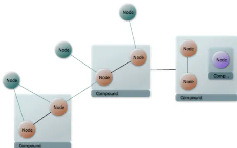
2.2 A compound graph with multiple levels of nesting . . . 9

2.3 Graph representation of a social network [4] . . . 10

LIST OF FIGURES xii

2.5 Visualization of the same graph before (left) and after (right)

ap-plying layout . . . 11

2.6 Visualization of a complex biological pathway(Activation of Cas-passes 3 and 7) using PATIKAweb [5] . . . 12

2.7 Same biological pathway with (Figure 2.6) after applying collaps-ing operations . . . 13

2.8 Graph visualization with fisheye view [6] . . . 14

2.9 Folding operation on a graph . . . 15

2.10 Hiding and ghosting operations on a graph . . . 15

2.11 Visual representation of SBGN [7] . . . 18

2.12 SBGN Process Description describing metabolic pathways of MAPK cascade [8]. . . 20

2.13 An example SBGN-PD map (left) and its SBGN-ML code (right) 21 2.14 Architecture of Cytoscape.js [9] . . . 23

2.15 Initialization of a simple graph using Cytoscape.js . . . 24

2.16 Graph model of Cytoscape.js . . . 25

2.17 A sample view from PCViz . . . 27

2.18 Two cancer studies are loaded to the network of MDM2 neighborhood 28 2.19 PCViz Architecture . . . 29

2.20 Compound structure problem with CySBGN . . . 32

2.21 Desired look of a node with auxiliary units (left), CySBGN look of nodes with auxiliary units (right) . . . 32

LIST OF FIGURES xiii

2.22 VISIBIOWeb is a web based tool to analyze SBGN-PD maps . . . 33 2.23 Members of a compound node must be inside it (left), dragging

causes misbehavior (right) . . . 34 2.24 Biographer can be used to import, export, edit and create SBGN

diagrams for all of its specifications . . . 35 2.25 SBGN-ED is a VANTED plugin used to analyze SBGN diagrams 36

3.1 A complex network visualization looks like an hairball with lots of edge crossings [10] . . . 38 3.2 The visualization of ATM mediated phosphorylation of repair

pro-teins in the context of MRN complex. . . 39 3.3 Traditional filtering techniques produce an inconsistent graph

(left), while the desired graph is a valid, complete SBGN map (right) . . . 40 3.4 A complex and a neighbor process (with orange border) are asked

to be expanded (left). First, all of their children are added to the expansion (right). . . 42 3.5 All of the parents of current node group are added to the expansion

because of the 4th _{principle (left), all components of the complexes}

are added to the expansion because of the 5th _{principle (right). . . 43}

3.6 Current expansion have processes (in blue) and neighbor processes (in red) to add their neighborhood to the expansion. . . 44 3.7 All of the neighborhood of the processes and neighbor processes

LIST OF FIGURES xiv

3.8 Newly added nodes might be in another parent or they might have children. So, we must add the parents (left) of the current ex-panded nodes considering the 4th _{principle. Also, these parents}

might have another children, we add the children of complexes again because of the 5th principle and complete expansion process

(right). . . 45

3.9 Expanding non-selected nodes (those inside blue box) would ex-pand them with unwanted nodes (those with orange border) . . . 46

3.10 The node group to be removed is orange (left), undesired part of the network is in green box and desired part is in blue one after the expansion of remaining nodes (right) . . . 47

3.11 Expansion of the desired part of the network (blue box in Fig-ure 3.10 (right)), the blue box includes the nodes to be shown . . 48

3.12 Active RAS is asked to be removed (left), outcome of this operation in the network (right) . . . 49

3.13 Inactive RAS is asked to be shown (left), outcome of this operation in the network (right) . . . 50

3.14 Active Grb2 is asked to be highlighted with its processes (left), outcome of this operation in the network (right) . . . 51

3.15 Active Grb2 is asked to be highlighted with its neighbors (left), outcome of this operation in the network (right) . . . 52

4.1 A sample view from SBGNViz.js-SA . . . 55

4.2 Detailed information of IRF1 is fetched from BioGene . . . 57

4.3 SBGNViz.js-SA architecture . . . 58

4.4 A process is selected (in magenta) and its details are shown in Details tab. . . 59

LIST OF FIGURES xv

4.5 Users click the edge between TP53 and MDM2 to see their detailed process in SBGN. . . 60 4.6 Detailed process information between MDM2 and TP53 in

SBGN-PD notation. . . 61 4.7 Filtering out the processes of NCI Nature from the SBGN-PD

Chapter 1

Introduction

A graph is a way of representing a set of objects (nodes) and relations (edges) between these objects. It is a data structure that could be used to model complex relational information such as network, communication, and data flow represen-tation. Using graphs as a formal way to visualize relational information eases data validation, integration, querying, and visualization.

Although, textual representation of relational information is simple and straightforward, it generally obstructs deriving information (Figure 1.1). Visual-ization of information has become a considerable aspect for understanding any kind of information (Figure 1.2). Information visualization counts on the human eye’s broad bandwidth pathway and offers techniques for representation of ab-stract information to allow people to see, explore, and understand large amounts of data at once and in intuitive ways [11].

The study and analysis of interaction between biological entities with networks has become a major area in bioinformatics (Figure 1.3). Many of the processes known to take place in biological cells are analyzed in the form of different types of networks [12]. The network complexity increases with new information pro-duced about these processes, which leads to difficulties of analyzing and retrieving information.

Figure 1.1: Textual representation of a biological pathway (Recruitment of repair and signaling proteins to double-strand breaks) in PathwayCommons [1]

Figure 1.2: Visual representation of a biological pathway (Recruitment of repair and signaling proteins to double-strand breaks) in PathwayCommons [1]

Figure 1.3: Visualization of a biological pathway (ATM Mediated phosphoryla-tion of Repair Proteins) in ChiBE [2]

Systems Biology Graphical Notation (SBGN) [13] has been developed by bio-chemists, modelers, and computer scientists to standardize biological pathway visualization so that scientists could represent biological pathways in a standard and unambiguous way. SBGN supports regularity, eliminates ambiguity, and fa-cilitates software support for transmission of complex information like well known standard visual languages such as Unified Modeling Language (UML) and Data Flow Diagrams. SBGN is formed by three languages (process description [14], entity relationship [15], and activity flow [16]), among which process description diagrams are arguably most commonly used ones in biology.

As mentioned earlier, size of the information to be visualized could be exces-sive and cause problems to understand information. The increase in the size of the information (e.g., size of information databases and the complexity of their structures) to be visualized forces a demand for more sophisticated complexity management techniques for many applications [3] (Figure 1.4). Showing, hiding, and emphasizing some parts of visualized network could dramatically increase the human comprehension over the visualization (Figure 1.5).

Figure 1.4: A complex real-life graph from software modeling [3]

Figure 1.5: Left: A map of a computer network after a series of complexity management operations applied. Right: The same network with certain desired parts revealed for detailed analysis. [3]

1.1

Motivation

Many graph visualization software have been developed to visualize pathway in-formation. While some of these tools are used for simple network visualiza-tion [17, 18, 19], there are also other alternative tools that support SBGN dia-grams [20, 21, 22, 23, 24, 25]. However, most of these tools are desktop appli-cations [21, 23, 26, 25] or plugins for desktop appliappli-cations [24]. Despite the fact that there are web based tools that support SBGN [20, 22], they do not sup-port interactive editing [22] or not available on touch enabled devices [20]. More importantly these tools also lack full support for compound structures used in representing molecular complexes and cellular locations / compartments.

In recent years, biological network data exchange format (BioPAX [27]) and biological pathway visualization standards (SBGN) have been developed and they take advantage of advanced graph visualization, including compound structure. All these reasons led us to research and development of visualization and com-plexity management of complicated biological networks.

Web based technologies have gained importance in recent years and became commonplace in software development. Along with the development of computing and storage technologies, users now heavily depend on online services. Besides that, web based software which has native browser support and does not depend on third party applications (like Flash) is platform independent and users do not need to install any other software. Those advantages make web based technologies an appropriate candidate to provide services to end users.

With the introduction of touch enabled mobile devices and computers, users have new possibilities to interact with software and applications. Touch feature required specialized software and hardware in the past, however, nowadays a lot of manufacturers offer devices and software supporting these new input meth-ods [28].

1.2

Contribution

Considering the complexity and the domain of biological pathways and underly-ing information, we determined the principles and invariants to properly manage complexity in SBGN-PD diagrams. Then, considering these principles and in-variants, we proposed algorithms to apply complexity management operations that involve showing, hiding, and emphasizing certain parts of a network without destroying the integrity of the pathway. These algorithms can be used when the user selects an entity group and applies any complexity management operation or when managing complexity according to an arbitrary domain knowledge is necessary.

We also developed an extension to Cytoscape.js (an open-source JavaScript graph library for analysis and visualisation) [9], called SBGNViz.js, to be able to visualize PD diagrams. This extension includes a converter from ML [29] to JSON since Cytoscape.js only accepts the JSON format and SBGN-ML generator to export the current network in SBGN-SBGN-ML format. Additionally, SBGN-PD entities can have dynamic data as described in section 2.3.2.

SBGNViz.js has the advantage of being written purely in JavaScript and in-herits support for touch enabled devices from Cytoscape.js, enabling use in a wide variety of devices, from a mobile phone to a desktop computer with a web browser. Also, SBGNViz.js is highly portable, thus a developer could easily use SBGNViz.js in any web-based application.

We also created a sample application, called SBGNViz.js-SA, to show the functionalities of SBGNViz.js and how easy to port it into a web application. SBGNViz.js-SA takes biological pathways to be visualized in SBGN-ML file for-mat and display it in SBGN-PD notation. SBGNViz.js inherits features of Cy-toscape.js scrolling, zooming, hiding and deleting facilities as well as its support for compound structure for compartments and complexes in SBGN. More im-portantly, we implemented complexity management operations that we designed. Furthermore, users could access gene-specific information from EntrezGene [30] through BioGene [31] facility.

Lastly, we integrated SBGNViz.js into PCViz [32], an open-source web-based network visualization tool that helps users query Pathway Commons [1] and ob-tain details about genes and their interactions extracted from multiple pathway resources. Users are able to see the neighborhood of a gene and select an interac-tion between a pair of genes to see its detailed pathway visualizainterac-tion in SBGN-PD format on a separate window.

Chapter 2

Background And Related Work

2.1

Graph Visualization

A graph G = (V, E) consists of a set of vertices V and edges E. An edge e ∈ E is a pair of vertices (u, v) where u ∈ V and v ∈ V are the endpoints of the edge. An edge associates its endpoints (Figure 2.1).

In a directed graph, every edge e = (u, v) has direction from u ∈ V to v ∈ V where u is the source vertex and v is the target vertex. However, there is no sense of direction for the edges in an undirected graphs.

Figure 2.1: A graph topology where a, b, c, d, e, f, g are vertices and the lines that connect the vertices are the edges.

If there is an edge e = (u, v) where u = v, that edge is called a loop or self edge. Two or more edges connecting the same source and target vertices are called multi-edges.

An edge e is in the outgoing edge list of a vertex u if u is the source of e; similarly, e is in the incoming edge list of a vertex u if u is the target of e.

A graph is called a compound graph if it contains any vertex that in turn includes nodes or edges inside (Figure 2.2). Compound graphs have child-parent relationship such that a compound vertex v is the parent of the vertices inside of v and every node inside of vertex v is a child of vertex v. A child node might in turn be a compound node giving opportunity to define multiple levels of nesting (Figure 2.2).

Figure 2.2: A compound graph with multiple levels of nesting

Graphs are used to define topological structure of relational information and they do not provide any geometric information for visualization. However, vi-sualization of a graph is a vital concept for users to understand the underlying information in a graph. Since the size and the complexity of information to be analyzed has been vastly increasing, graph visualization techniques are needed even more for analysis (Figure 2.3 and Figure 2.4).

Figure 2.3: Graph representation of a social network [4]

for graph elements such as location, width, height, and border along with its topological structure. Many cosmetic properties like color, transparency, border shapes, edge arrow shapes are also considered aspects of graph visualization. In fact, any visual concept that influences viewers’ comprehension is treated as a graph visualization concept.

Layout of a graph corresponds to its geometry, aiming visualization with aes-thetically pleasing results. Although the aesthetic quality of a visualization might change from one to another, there are some certain aspects to consider while ap-plying layout like minimizing edge crossing number, total drawing area, total edge length and increasing uniformity of edge length and reflecting the topologi-cal symmetry of the graph. A graph visualized with a bad layout could confuse users whereas a good layout would help to understand the underlying information and its topology (Figure 2.5).

Figure 2.5: Visualization of the same graph before (left) and after (right) applying layout

2.2

Complexity Management in Graph

Visual-ization

Complex relational information such as biological and social networks are gen-erally too large to visualize at once and details become hard to detect resulting in extra effort of users to understand the network. In visualization of graphs,

masking unwanted parts of the network and unmasking those parts when needed are the strategies called complexity management techniques. The techniques like hiding, folding, ghosting, and nesting have an important role on visualization of biological networks as well as any other domain.

The practicality of complexity management techniques is variant in the con-text of the information to be visualized. For example, hiding a child of a com-pound node is not a good way to manage the complexity if the comcom-pound node is only complete with its components and might have different type or meaning in its new state. This will be discussed in more detail later in Section 3.1. After all, some complexity management operations could not be applied blindly without considering the domain knowledge.

A common complexity management technique for graphs with nested topol-ogy is collapsing a compound node. It simply shows a compound node as a simple node and creates meta edges for the node’s children. Using this method, a com-plex graph (Figure 2.6) could be simplified and currently unnecessary parts of the topology could be made insignificant in a reversible way (Figure 2.7).

Figure 2.6: Visualization of a complex biological pathway(Activation of Caspasses 3 and 7) using PATIKAweb [5]

Figure 2.7: Same biological pathway with (Figure 2.6) after applying collapsing operations

Another popular complexity management technique, called fisheye view, scales up the center of the view decreasing the level of details towards the boundaries of the graph [33]. Thus, the user could emphasize the area of interest of the graph (Figure 2.8). This technique can be used in real time as users change the area of interest and focus point is updated smoothly and simultaneously.

Folding operation creates a new folder node and puts a group of graph mem-bers inside of the folder node. The folder node is a simple node and created in collapsed mode to decrease the graph size. Using this method, currently un-wanted parts of the network can be collapsed in a folder node, allowing to reverse the operation on demand by unfolding the node. Also, it can be used to group the graph components according to some criteria.

Figure 2.9 shows an example of folding operation on a graph. The nodes in dark blue are asked to be folded in a node and the result of that operation is on the right. Dark blue nodes and their edges are placed in a newly created folder node. Meta edges are created between folder node and the rest of the graph, representing the edges of nodes a and b whose one end is inside the folder.

Figure 2.8: Graph visualization with fisheye view [6]

Hiding operation could be applied to a graph member by not rendering it on the display. In that case, the graph member is not displayed in the current network and it is removed from the graph topology, thus users are unable to interact with it.

Ghosting technique could be used to deemphasize a graph member by chang-ing its visual style like opacity, color, and brightness. Ghostchang-ing does not remove any graph member from the graph and the topology, it only looses the focus on the ghosted graph member and users are able to interact with it.

Figure 2.10 shows an example of hiding and ghosting operations. Nodes a, b, and their incident edges are hidden in the graph. Additionally, compound node c and its children with their incident edges are ghosted i.e., transparency of these nodes is increased.

Figure 2.9: Folding operation on a graph

2.3

Systems Biology Standards

2.3.1

BioPAX

BioPAX, short for Biological Pathway Exchange, has been developed as a standard language to represent biological pathways at molecular and cellular level [27]. It covers a variety of pathways from signalling to ppi networks. In recent years, plenteous amount of pathway data has been generated by diverse communities. Such a development has conceived huge databases and many tools for utilization of pathway information. However, diversity of tools, databases and notation across communities have caused inefficiency because of the lack of data integrity. To overcome this problem, BioPAX has been introduced as a standard to collect, index, interpret and share pathway information. By courtesy of BioPAX, a huge amount of pathway data from many types of organisms is now available from an expanding number of databases.

2.3.2

Systems Biology Graphical Notation (SBGN)

Biology is one of the fields that have highest rate of graphical and textual informa-tion. Although BioPAX filled a gap in storing and formatting of biological infor-mation, there was still an ambiguity of a standard graphical notation. To resolve this problem, Systems Biology Graphical Notation (SBGN), a visual language developed by a community of biochemists, modelers, and computer scientists, was introduced [13].

While developing SBGN, scientist’s major concern was to cover almost all technical and practical needs of the diverse biology community. Therefore, SBGN is an open source project, and is still improved by a large community. Common biological objects, their properties and interactions from different biological com-munities are visually supported with this notation. SBGN is in favor of keeping notation, number of objects and syntax at a minimum level to increase learning curve and comprehension of users. Also, it is highly modular to handle large

diagrams and complexity easily.

Interactions between biological entities differentiate with their properties. It is useless and vain to represent all reactions and interactions in the same dia-gram, resulting in incomprehension and confusion. To solve this problem, three different styles of notation has been introduced, Process Description [14], Entity Relationship [15], and Activity Flow [16], to represent only required interactions of a specific context. Our focus and work was on Process Description (Figure 2.11) diagrams since it is widely used by the biology community.

Figure 2.11: Visual represen tation of SBGN [7]

A process diagram represents all the molecular processes and interactions taking place between biochemical entities and their products [13]. Change is the aspect of process description describing how entities are processed from one form to another.

Entity Pool Node (EPN) represents any physical or conceptual entity in a bi-ological network. The PD includes six EPN that represents physical entities: un-specified entity, simple chemical, macromolecule, nucleic acid feature, multimer, and complex. Additionally, source, sink, and perturbing agents are conceptual entities in PD.

EPNs could contain auxiliary units that provide additional information. They are placed on the boundaries of the EPN.

• Unit of information is used to show abstract information related to the functionality of the entity it belongs to.

• State variable shows current state of the entity, corresponds to physical or informational configuration.

• Clone marker shows whether the entity is cloned, indicates that another occurrence of that entity can be found in the map.

EPNs are transformed to other EPNs by processes. Different process types are represented with process, omitted process, uncertain process, association, dis-sociation, and phenotype as seen in Figure 2.11.

Complex and Compartment are compound nodes in PD maps. Complex node represents an entity that consists of a number of other entities. A complex has its own identity and must be considered with all of its components. Compartment node represents a logical or physical structure composed of entity pool nodes.

For example, in Figure 2.12, RAF macromolecule and ATP enter a process with the catalysis RAS macromolecule in active state and leave as phosphorylated RAF and ADP. As it is seen, the overall diagram shows how entities are changed by different processes.

Above, we gave an overview of Process Description language. Further details could be found in Process Description language Level 1 documentation [14].

Figure 2.12: SBGN Process Description describing metabolic pathways of MAPK cascade [8].

Although SBGN standardizes representation of biological pathway informa-tion in a concise and unambiguous way, it does not offer any standard for how the maps should be stored. Because of that, the biological maps produced by any tool could not be used in another. To overcome this problem, SBGN-ML, a dedicated, lightweight XML-based file format, was developed[29]. SBGN-ML includes all necessary information to draw the entities in SBGN and stores the positions of entities, i.e., layout of the maps (Figure 2.13).

Figure 2.13: An example SBGN-PD map (left) and its SBGN-ML code (right)

2.4

Related Software

In this section, we will go over related software tools.

2.4.1

Cytoscape

Cytoscape family has three visualization software, Cytoscape, Cytoscape Web, and its successor Cytoscape.js.

Cytoscape [34] is an open source desktop application to visualize molecular interaction and biological networks and integrate these networks with additional data like annotations and gene expressions. Cytoscape was developed for bio-logical research but it is a general platform for complex network analysis and visualization nowadays. It offers lots of features for data integration, analysis, and visualization.

Cytoscape Web is a web based graph visualization library that depends on Flex / ActionScript technologies. It can be easily embedded to any web appli-cation. Additionally, Cytoscape Web offers a JavaScript API to customize and manipulate the network at client side.

Cytoscape.js has been developed as an open source graph library written in JavaScript, utilized for analysing and visualizing graphs. It does not depend on any third-party application like flash and also supports mobile browsers. Along with all the features of Cytoscape Web, it offers new queries for data management and takes advantage of latest web technologies. It is funded by NRNB (Natural Resource for Network Biology) [35] and NIH (National Institutes of Health) [36]. The main difference between Cytoscape’s web and desktop applications is that Cytoscape is an application for end users, whereas Cytoscape web applications require to write code using their API.

Cytoscape.js gives users an opportunity to display and manage graphs inter-actively. It supports both desktop and mobile browsers; thus, it allows users’ interaction with graphs, such as selection, pinch-to-zoom, and panning for both touch and non-touch operated devices.

Cytoscape.js depends on event-driven model with a core API [9] (Figure 2.14). The core is the component that offers functions to change the graph as a whole, like applying layout and panning the graph. Also, it provides lots of functions for efficient access of graph elements. Additionally, it has some extensions and is responsible to notify the extensions when needed. Extensions make the necessary changes on graph elements and notify the core about the changes. The extensions are non-transparent to the client applications, as clients access Cytoscape.js only through the core using its API.

Figure 2.14: Architecture of Cytoscape.js [9]

Cytoscape.js gets graph elements and their style properties, layout options, and any other graph property as JSON objects during initialization (Figure 2.15). Style properties follow CSS convention and Cytoscape.js introduces its own style properties in case CSS properties are insufficient.

Another strong side of Cytoscape.js is that it contains lots of graph analysis algorithms from graph theory such as breadth first search, depth first search, minimum spanning tree and Dijkstra’s shortest path. Users are able to obtain and operate on neighborhood, connected edges, descendants, children, parents, siblings, etc. of a node group with a single function.

Cytoscape.js provides full support for compound structures and offers useful functions to access, traverse, and perform operations on compound nodes. This support makes Cytoscape.js convenient to use in domains where hierarchically structured information needs to be visualized.

Cytoscape.js adopts the selector facility of JQuery [37] and selectors work on graph elements. It greatly simplifies traversing and manipulating the nodes according to some criteria. For example, the user could apply breadth first search

Figure 2.15: Initialization of a simple graph using Cytoscape.js

on nodes with weight higher than a number, get all descendants of a compound node with a certain shape and logically combine a couple of criteria together. Besides, those functions are chainable, users are able to call several functions on the same graph element consecutively. For example, to get all complexes’ macromolecule children, the user can apply the following function:

cy.nodes(”node[class=’complex’]”)

As it is seen, selectors and chaining are very useful to apply complexity man-agement operations on SBGN diagrams.

Cytoscape.js stores the elements (nodes and edges) in an array structure and uses a map structure to access the elements using their ids. For parent-child relationship, the parent has an array list of children kept consistent with the graph state. Accessing an element using its id takes O(logN ), where N is the size of the element array. Also, iterating over elements array costs O(N ).

The core of Cytoscape.js offers a couple of functions to access the elements in the graph. These functions return a Collection, which stores a set of elements in the graph. Additionally, collections offer a set of functions to filter, edit, and traverse the collections. Most iteration operations, if not all, cost O(N ) on the list itself but O(1) for accessing the list.

Figure 2.16 shows the class diagram that summarizes graph model of Cy-toscape.js. Since Cytoscape.js does not have object-oriented design, this diagram does not show the actual architecture but gives the overall design approach.

Cytoscape.js offers a couple of functions to layout graphs. Users are able to choose a suitable layout algorithm according to the context of their graph. Grid, Breadth First, Arbor [38], Preset with predefined positions, and CoSE [39] are some of the layout algorithms that Cytoscape.js support.

2.4.2

Pathway Commons

Pathway Commons [1] is a service that provides publicly available pathway infor-mation of various organisms. It includes several database sources which support BioPAX format for biological pathways. Biologists can use web interface of Path-way Commons’s to access an extensive amount of biological data. They can specify a gene set and the type of the query such as paths between and neighbor-hood and obtain the pathway data in various format such as SBGN-ML, BioPAX, and Simple Interaction Format (SIF).

2.4.3

PCViz

PCViz [32] is an open source web based network visualization tool that offers to make queries to Pathway Commons to retrieve biological pathway information for a set of genes from several pathway data providers. It uses these queries to visualize networks of interaction and acquire information about gene details (Figure 2.17).

PCViz provides lots of features and advantages for biological network analysis and visualization. PCViz

• is compatible with almost all web-browsers, including the ones on the mobile devices (e.g., iPad and devices with Android OS).

• is only human-oriented, does not include information about other organ-isms.

Figure 2.17: A sample view from PCViz

• uses Pathway Commons data to be able to visualize thousands of genes and their interactions.

• allows to add new genes of interest to the current network of interest. • takes advantage of full BioPAX representation and extract relevant

infor-mation from the complex BioPAX data coming from Pathway Commons. • reduces the size of the network by filtering genes or interactions based on

different criteria like interaction type, more relevant genes with the genes of interest

• allows users to load multiple cancer contexts to the network to see the overall frequency of alteration for each gene and uses this information to enhance the complexity management. For instance, when cancer context is

loaded, the nodes that have low frequency of alteration are filtered first.

As mentioned before, PCViz provides cancer context information. It uses cBioPortal [17] to retrieve cancer information about the genes in the network. After the network is loaded, users can get a list of all cancer studies and select one study and get a list of all genomic data types available. When the cancer data is loaded to the network, PCViz represents this data via visual styles, e.g. from gray to red gradient color on the nodes (Figure 2.18).

Figure 2.18: Two cancer studies are loaded to the network of MDM2 neighbor-hood

Figure 2.19 shows PCViz architecture and summarizes its features. Back-end of PCViz

• is implemented with Springs MVC framework as a REST service. All ser-vices provide data in JSON format to the client side. Queries are cached on the backend side to reduce lag for queries.

• retrieves pathway information of specified genes of interest in BioPAX for-mat.

• makes a query to BioGene and retrieve the gene information in JSON format when users click to a gene.

• makes a query to iHOP and retrieve edge annotation data in text format when users click to an edge.

• makes a query to cBioPortal and fetch cancer study to be loaded in TSV (tab seperated value) format.

Figure 2.19: PCViz Architecture

Back-end of PCViz converts all data to JSON and passes it to front-end. PCViz’s front-end

• is responsible to render the view of PCViz.

• generates a canvas for SIF view and SBGN view using Cytoscape.js. It uses Backbone.js to structure the view by defining gene names as model and Cytoscape.js instance on the html dom object as view component. The network information from Pathway Commons is retrieved in the Backbone instance using the genes of interest.

• generates Details view in the tabbed menu (Figure 2.18). When users click a gene, it renders the BioGene information of this gene using Backbone.js. It uses Backbone.js as SBGNViz.js-SA uses. Additionally, when users click an edge, it makes a query to iHOP and shows edge annotation data. • generates Settings view. This view offers filtering according to the

interac-tion types and a smart filtering opinterac-tion that filters the nodes according to relevance with the genes of interest.

• generates Context view. When users select a cancer study, it makes a query to cBioPortal and retrieve the alteration frequencies of the genes in the network.

2.4.4

Paxtools

BioPAX, as mentioned earlier, encapsulates a huge amount of pathway data and genetic, protein interactions. Since BioPAX includes massive number of classes and properties, it is grueling to produce and modify such data. Paxtools sorts this problem out by introducing a java API that transforms BioPAX properties to Java classes, offering methods and algorithms for utilization of BioPAX proper-ties. Such methods include reading, writing, searching, merging, comparing, and transforming pathway information and help scientists to access and use BioPAX data with proven software since Paxtools is developed by the community [40]. With lots of pathway data providers that support BioPAX, scientists can easily access data and use it within their software tools for visualization, validation, and analysis.

2.4.5

BioGene

BioGene [31] is a simple web service where scientists can query a gene and retrieve information about its functions and references. It primarily uses Entrez Gene, a gene database provided by NCBI [30].

2.4.6

cBioPortal

cBioPortal is a web application that allows users to explore, visualize, and analyze cancer genomics data [17]. Given a set of gene and associated cancer study, it visualizes the network with alteration frequencies caused by the cancer study in question. It uses Adobe Flash Based CytoscapeWeb for visualization and cannot be used in mobile devices.

2.4.7

CySBGN

CySBGN is a Cytoscape plugin that lets users import, modify, and examine SBGN Diagrams [24]. Since Cytoscape is a desktop application, it can not be used online, however it supports all major operating systems: Linux, Windows and MacOs X.

Unfortunately, CySBGN does not support all edge and node shapes in SBGN-PD. It makes its own conventions for shapes that Cytoscape does not support. Also, it is not compatible with the latest version of Cytoscape and does not support compound nodes. Complexes and compartments are drawn with trans-parency to represent parent-child relations. When the user moves a child, it might jump out of the compound node in a way that violates the compound structure (Figure 2.20). Also, some Cytoscape features like layout can not be applied to any SBGN-PD diagrams since it will ignore the nesting structure.

Another problem with CySBGN is that, it does not have z-index ordering for nodes. That causes a problem when rendering a node with auxiliary units, since

Figure 2.20: Compound structure problem with CySBGN

they are rendered as other nodes and connected to its node with an edge. In other words, a node might be rendered with its auxiliary units behind it, resulting in unpleasant layouts (Figure 2.21).

Figure 2.21: Desired look of a node with auxiliary units (left), CySBGN look of nodes with auxiliary units (right)

2.4.8

VISIBIOweb

VISIBIOWeb [22] is a free web service that is used for visualization and layout of BioPAX pathway models (Figure 2.22). It depends on JavaScript and Google Maps API [41] and shows a static image of the pathway in SBGN-PD format, allowing use in both mobile and desktop browsers. It only accepts “.owl“ type files to load and analyse, however users are able to export the network in SBGN-ML format.

VISIBIOWeb does not allow users to edit the geometry or the style of the graph elements since it displays a static image of the pathway; in other words,

Figure 2.22: VISIBIOWeb is a web based tool to analyze SBGN-PD maps the visualized network can not be edited interactively. However, nodes could be clicked on to show their properties as extracted from associated “.owl“ file. Addi-tionally, basic graph visualization concepts like zooming, panning, and scrolling are also possible.

2.4.9

Biographer

Biographer is a comprehensive tool developed by Theoretical Biophysics Group in Berlin and used for visualization and layout of biological networks [20]. It is formed by three components, layout component written in C++, JavaScript web component for visualization and server component that composes those compo-nents and provides network import and visualization.

model. It builds up a layout for overall positioning of the networks, making use of hierarchical model for layout of individual reactions. Hierarchical layout puts substrates at the top and products at the bottom, placing other entities to the left and the right.

Unfortunately, compound structure support of Biographer is not complete. Although layout component takes compound entities of SBGN into account, user interaction with compounds does not go with the grain. When a user drags a compound node, its children also move within it. However, child node goes out of the boundaries of its parent in case of dragging, making it look like there is no child-parent relation between them (Figure 2.23). Additionally, users need to adjust width and height of SBGN compound structures manually to be able to add children.

Figure 2.23: Members of a compound node must be inside it (left), dragging causes misbehavior (right)

Biographer also provides an online editor for all of three specifications of SBGN. Users are able to create their diagram with lots of customization options (Figure 2.24).

Figure 2.24: Biographer can be used to import, export, edit and create SBGN diagrams for all of its specifications

2.4.10

SBGN-ED

SBGN-ED [21] is an extension of VANTED (Visualisation and Analysis of Net-works containing Experimental Data) developed to create, edit, visualize, and validate SBGN maps (Figure 2.25). It supports all three types of SBGN.

VANTED [42] is an open source, desktop application, that provides loading, editing, and analyzing graphs with biological pathway information or functional hierarchies. VANTED and SBGN-ED can not be used online but works on all major operating systems with Java support.

Beyond visualization of SBGN-PD diagrams, SBGN-ED offers functional-ity for data mapping and processing, and statistical analysis. The features of VANTED and its add-ons are also available for SBGN-ED, allowing users to broaden the functionality of the software.

Figure 2.25: SBGN-ED is a V ANTED plugin used to analyze SBGN diagr ams

Chapter 3

Methods For Visualizing

SBGN-PD Maps

3.1

Motivation

As mentioned before, biological pathways are generally too large to visualize and details become obscured. Such networks can be reduced temporarily by removing or understating the currently unnecessary parts of a network; such examples have been provided in Section 2.2.

The core of an SBGN-PD diagram is processes and their interactions. Al-though pathway data is accessed from databases with sophisticated and context-related queries, such biological information might contain thousands of molecular entities. Excessive amount of data restricts the capabilities and features of net-work visualization tools. Visualization of such netnet-works ends up being slow on interactive analysis and graphs look like an hairball because of the great num-ber of edge crossings (Figure 3.1). Using complexity management operations like hiding or folding unwanted parts of the graph and abstraction of the network in various layers could dramatically lower the size of such network diagrams, allowing effective visualization.

Figure 3.1: A complex network visualization looks like an hairball with lots of edge crossings [10]

These complexity management techniques fall behind when context and char-acteristics of process description diagrams are taken into account. It is crucial that the overall integrity and validation of a biological process network should not be destroyed while hiding or filtering some parts of that network. For example, a process node must be filtered out if all of its substrates, products and effectors are also filtered out. Otherwise, the diagram will remain in an inconsistent state. For example, users might make a query to show only NBN proteins on such a network in Figure 3.2. Applying traditional techniques would end up with inconsistent results. As it is seen in Figure 3.3 (left), processes and their edges are cleared away and reaction information is lost. Additionally, some of the components of the complexes are removed although complexes have their own identity with their components. Consequently, a general complexity management technique would violate the underlying information and the characteristics of the entities.

Considering the characteristics of SBGN-PD, we need to transform the query to ”show only processes that involve NBN proteins”. Such a query would give consistent results without violating SBGN-PD rules as seen in Figure 3.3 (right).

Figure 3.2: The visualization of ATM mediated phosphorylation of repair proteins in the context of MRN complex.

We intend to define all characteristics of SBGN-PD to be able to manage complexity in large biological networks. Considering these characteristics, we introduce new algorithms to be able to modify all types of general complexity management techniques to keep the SBGN-PD maps intact and consistent when these operations are applied to such diagrams. Additionally, we propose some techniques to manage complexity according to an arbitrary domain knowledge.

Figure 3.3: Traditional filtering techniques produce an inconsistent graph (left), while the desired graph is a valid, complete SBGN map (right)

3.2

Complexity

Management

of

SBGN-PD

Maps

Complexity management operations on SBGN-PD maps generally work in a way that shows, hides or emphasizes a part of the network. Those operations are generally applied to a node group that is a set of entities in a biological network. Unfortunately, as mentioned above, complexity management cannot be done by only showing or hiding such a node group. For example, a process must be considered with all of its inputs and outputs. Thus, hiding only one process has no meaning (some of the entities might be in the map to represent the hidden process). Similarly, hiding a subset of a complex’s members will leave the network in an invalid state.

To overcome this problem, we have the following principles / invariants to satisfy when showing or hiding a node group:

1. If a node has to be shown, it should be displayed.

with should be displayed since SBGN-PD shows the transformation of these biological entities via processes.

3. If a process has to be shown, then all of its inputs, outputs, and effectors should be displayed too. A process shows the transformation of the biologi-cal entities and hiding an input, output, or effector might refer to a different kind of process. Additionally, hiding an input produces inconsistent results since the outputs are formed according to the inputs.

4. If a node has to be shown, the parent node (complex or compartment) should be displayed since the complexes are identified with their components and compartments represents the logical or physical structure that is formed by its components.

5. A complex molecule should always be displayed with all of its components since a complex represents a biological entity composed of other biological entities and the resulting entity has its own identity.

To be more clear, the 5th _{principle partially applies to the same for}

compart-ments. If a compartment is in the node group to be shown, obviously, all of its components must be displayed too. However, some of the nodes in the node group to be shown might be in a compartment without the compartment itself being in the specified group. In that case, only those nodes must be shown, not all of the components of the compartment. In contrast, all of the complex’s components must be displayed no matter what.

Thus, when a complexity management operation is performed on a node group, the group must be expanded according to the principles described above. Expanding a node group indicates adding other nodes (in the neighborhood of the node group and need to be added according to the principles) to the node group. We propose expandNodes algorithm to solve this problem (Algorithm 1).

Algorithm 1 Expanding node group according to SBGN-PD criteria procedure ExpandNodes(nodeGroup)

nodeGroup = nodeGroup ∪ nodeGroup.descendants() nodeGroup = nodeGroup ∪ nodeGroup.parents()

nodeGroup = nodeGroup ∪ nodeGroup(”complex”).descendants() processes = nodeGroup(”process”)

nonProcesses = nodeGroup(”!process”)

neighborProcesses = nonProcesses.neighborhood(”process”)

nodeGroup = nodeGroup ∪ processes.neighborhood() ∪ neighborProcesses ∪ neighborProcesses.neighborhood()

nodeGroup = nodeGroup ∪ nodeGroup.parents()

nodeGroup = nodeGroup ∪ nodeGroup(”complex”).descendants() return nodeGroup

end procedure

When a node group needs to be expanded (Figure 3.4 (left)), we first add all the descendants of the nodes (Figure 3.4 (right)).

Figure 3.4: A complex and a neighbor process (with orange border) are asked to be expanded (left). First, all of their children are added to the expansion (right). According to the 4th principle, we need to add all parents of the node group (Figure 3.5 (left)). Expanding the node group with parents might add new com-plex nodes, so we add all comcom-plexes’ components to the node group because of the 5th _{principle (Figure 3.5 (right)).}

Figure 3.5: All of the parents of current node group are added to the expansion because of the 4th _{principle (left), all components of the complexes are added to}

the expansion because of the 5th principle (right).

Until now, we expand the selection with parents and children of the node group according to the principles. Now, we need to define three different node groups:

• processes are all the processes in the node group, we need to add all of their neighborhood considering 3rd principle.

• nonProcesses are all the non-processes in the node group, we need their processes because of the 2nd _principle.

• neighborProcesses are the processes connected to nonProcesses and not in the node group currently.

Figure 3.6 shows these node groups with different colors; processes, nonPro-cesses, and neighborProcesses are in blue, orange, and red, respectively.

Figure 3.6: Current expansion have processes (in blue) and neighbor processes (in red) to add their neighborhood to the expansion.

Next, we need to add neighborProcesses and neighborhood of processes and neighborProcesses (Figure 3.7). Notice that, neighborProcesses and their neigh-borhood are added to the node group due to 2nd _{and 5}rd _{principles, respectively.}

Figure 3.7: All of the neighborhood of the processes and neighbor processes are added to the expansion.

Lastly, adding new nodes might bring new parents and complexes, so we add parents and components of complexes again (Figure 3.8). Finally, node group has been expanded without destroying the integrity of the network.

Figure 3.8: Newly added nodes might be in another parent or they might have children. So, we must add the parents (left) of the current expanded nodes considering the 4th _{principle. Also, these parents might have another children,}

we add the children of complexes again because of the 5th _{principle and complete}

expansion process (right).

The expandNodes algorithm can be used where users specify a node group and want to emphasize it somehow (showing, highlighting, etc.). Often times, user can specify a node group and emphasize the remaining nodes in the network (i.e., the specified node group might be deemphasized). In this situation, expanding the remaining nodes directly does not solve our problem. That approach might bring unwanted nodes back.

As it is seen in Figure 3.9, the user might ask to hide the selected nodes with orange border. Expanding the remaining nodes in blue box using expandNodes algorithm would result the entire graph to be in the node group after the ex-pansion according to the 2nd _{and the 3}rd _{principles. Phosphorylated RSK and}

phosphorylated ERK have a process in the node group to be hidden and this process must be hidden with all of its neighbors.

Figure 3.9: Expanding non-selected nodes (those inside blue box) would expand them with unwanted nodes (those with orange border)

We propose an expandRemainingNodes algorithm to be able to remove a node group properly, keeping the above principles in mind (Algorithm 2).

Algorithm 2 Expanding remaining node group according to SBGN-PD princi-ples

procedure ExpandRemainingNodes(nodeGroup, allNodes) nodeGroup = expandNodes(nodeGroup)

remainingNodes = allNodes.not(nodeGroup) remainingNodes = expandNodes(remainingNodes) return remainingNodes

end procedure

When a node group is somehow needed to be deemphasized, that group must be expanded first, in line with principles set forth. In other words, we could not directly hide them since they might contain entities from desired part of the network because of the expansion. For example, the node group to be removed might contain a macromolecule connected to a process from the network to be shown. As it is seen in Figure 3.10 (right), we could not remove phosphorylated RSK since it has a process within the desired part.

Figure 3.10: The node group to be removed is orange (left), undesired part of the network is in green box and desired part is in blue one after the expansion of remaining nodes (right)

In fact, the problem is that an entity in the graph could possibly participate in any number of processes. Some of these processes might be in desired parts of the graph, whereas some might not be. Users probably do not want to see a group of processes and the remaining processes should be complete. In order to achieve this, we use expandNodes algorithm again, but on the node group to be shown. In Figure 3.10 (right), the node group in blue box is the one to be shown and Figure 3.11 shows the final node group to be shown after expansion.

The expandNodes and expandRemainingNodes algorithms are the bases for complexity management techniques for SBGN-PD maps. In expandNodes al-gorithm, we get parents, descendants, and neighborhood of given set of nodes. Those node groups might end up making up the entire graph, so its worst-case running time is O(N ), where N is the number of nodes. The expandRemainingN-odes algorithm uses the expandNexpandRemainingN-odes algorithm twice, so its complexity is also O(N ).

In the next section, we present the actual complexity management techniques implemented in SBGNViz.js, using the algorithms described above. Other than expanding algorithms, they only perform delete or highlight of the nodes, which

Figure 3.11: Expansion of the desired part of the network (blue box in Figure 3.10 (right)), the blue box includes the nodes to be shown

cost O(N ) at the most.

3.2.1

Hide Selected Node Group

A node group could be selected and asked to be removed from the view. In that case, the expandRemainingNodes algorithm is applied to the selected node group. This algorithm returns the nodes to be shown in the network, so we hide the rest of the network (Algorithm 3).

Algorithm 3 Hide selected node group

procedure hideSelectedNodes(selectedElems) allElems are all of the elements in the map

elemsToShow = expandRemainingNodes(selectedElems, allElems) elemsToHide = allElems.not(elemsToShow)

hide(elemsToHide) end procedure

removed from the graph. Such a request would remove all of its processes and all neighbors of these processes. Since the complex node is in another process from the desired part of the graph, it stays in the node group to be shown with all of its components.

Figure 3.12: Active RAS is asked to be removed (left), outcome of this operation in the network (right)

3.2.2

Show Selected Node Group

A node group could be selected with the purpose of hiding the rest of the network. We need to use the expandNodes algorithm on selected nodes to obtain the nodes to be shown. After expanding nodes, we need to hide the rest of the network (Algorithm 4).

Algorithm 4 Show selected node group

procedure showSelectedNodes(selectedElems) allElems are all of the elements in the map

elemsToShow = expandNodes(selectedElems) elemsToHide = allElems.not(elemsToShow) hide(elemsToHide)

end procedure

selected node, only its processes and involvements are shown in the network.

Figure 3.13: Inactive RAS is asked to be shown (left), outcome of this operation in the network (right)

3.2.3

Highlight Processes of Selected Node Group

Highlighting a node group emphasizes the node group without removing anything from the network. It can be done in several ways according to the style conven-tions of the tool used. We simply assume the opacity of the nodes that are not in the node group to be decreased for this purpose.

Highlighting processes of selected objects includes highlighting all of the se-lected processes and immediate neighbors of these processes. In fact, it highlights exactly the same node group that the expandNodes algorithm returns (Algo-rithm 5).

Algorithm 5 Highlight Processes of Selected Node Group

procedure highlightProcessesOfSelected(selectedElems) selectedElems = expandNodes(selectedElems)

highlight(selectedElems) end procedure

be highlighted with its processes. Notice that, Grb2 itself is not directly involved in a process but its parent is a complex and 4th _{and 5}th _{principles enforce the}

selection to be expanded to include the complex.

Figure 3.14: Active Grb2 is asked to be highlighted with its processes (left), outcome of this operation in the network (right)

3.2.4

Highlight Neighbors of Selected Node Group

Highlighting neighbors of the selected nodes is different from other complexity management techniques as it partially supports the principles. Since we just want to highlight neighbors, the 3rd principle is omitted. If a non-process node is se-lected, only its processes are highlighted instead of highlighting all neighborhood of those processes. Such an operation would be helpful in a crowded graph where it is difficult to understand the neighbors because of edge crossings. Hence, we do not base our Highlight Neighbors of Selected Node Group algorithm on any expand algorithms (Algorithm 6).

First, complex parents are added to the node group since complexes must be considered as a whole. Then, we add descendants of these parents since they may contain other entities. These two steps are very similar to second and third step of expandNodes algorithm. Next, neighborhood of the node group and their descendants are added to the node group and highlight operation is applied.

Algorithm 6 Highlight Neighbors of Selected Node Group

procedure highlightNeighborsOfSelected(selectedElems) selectedElems = selectedElems ∪ selectedElems.parents(”complex”) selectedElems = selectedElems ∪ selectedElems.descendants() selectedElems = selectedElems ∪ selectedElems.neighborhood() selectedElems = selectedElems ∪ selectedElems.descendants() highlight(selectedElems)

end procedure

Figure 3.15 shows an example of this operation. Active Grb2 is asked to be highlighted with its neighbors. Since its parent is a complex, neighbors of that complex are also shown.

Figure 3.15: Active Grb2 is asked to be highlighted with its neighbors (left), outcome of this operation in the network (right)

3.2.5

Filter by Arbitrary Domain Knowledge

In addition to highlighting and filtering a user-selected node group, it is essential to apply such operations in the context of and in line with an arbitrary domain knowledge. For example, biological pathway data providers like Pathway Com-mons might offer biological pathways that include processes from various sources. Some sources might be thought to be highly reliable than others. Also, some bi-ological pathways have network-context information like alteration frequencies of

biological entities from a cancer study. Users should be able to eliminate less affected biological entities from a pathway map without destructing the map’s integrity. Such queries can be handled by using the expand algorithms described earlier on the node group to be shown or hidden according to the domain knowl-edge.

Chapter 4

Tools For Visualizing SBGN-PD

Maps

In this chapter, we present the software tools that implement our methods pre-sented earlier.

4.1

SBGNViz.js

SBGNViz.js [43] is developed as an extension of Cytoscape.js [9] to visualize bi-ological maps represented with SBGN Process Description language. Taking ad-vantage of Cytoscape.js visualization and gesture facilities, SBGNViz.js supports all node and edge shapes introduced in SBGN Process Description notation.

Cytoscape.js accepts extensions of several types. An extension can be a core, collection, layout or renderer extension. Since SBGNViz.js introduces new node and edge shapes, it registers to Cytoscape.js as a renderer extension.

Developers are allowed to add any property to nodes’ and edges’ data object in case the properties are needed for an extension. As explained before, along with the shape, dimensions and label of the entities of SBGN Process Description

notation, they have other properties like auxiliary units, multimer and port in-formation. Those SBGN-PD related properties are attached to nodes’ and edges’ data object as JSON objects to be used during initialization of Cytoscape.js and SBGNViz.js uses this data while rendering SBGN-PD node and edge shapes.

4.2

SBGNViz.js-SA

SBGNViz.js-SA [44], short for SBGNViz.js Sample Application, uses SBGNViz.js to visualize, analyze, and edit biological pathways represented in SBGN-ML (Fig-ure 4.1). Along with its support for basic graph visualization feat(Fig-ures like panning and zooming, it provides full compound structure support for compartments and complexes in SBGN-PD notation.

Figure 4.1: A sample view from SBGNViz.js-SA