On the effective bandwidth for resource management in ATM networks

ON TH E EFFECTIVE BAN PW IPTH

F O R lU S S O m C E BflANAGEMENT IN ATM

■•NETWORKS

A THESIS

SUBMITTED TO THE DEPARTMENT OF ELECTRICAL AND

ELECTRONICS ENGINEERING

AND THE INSTITUTE OF ENGINEERING AND SCIENCES

OF BILKENT UNIVERSITY

IN PARTIAL FULFILLMENT OF THE REQUIREMENTS

FOR THE DEGREE OF

MASTER OF SCIENCE

B y

T ija n i C h a h ed

J u n e 1 9 9 7

ON THE EFFECTIVE BANDWIDTH

FOR RESOURCE MANAGEMENT IN ATM

NETWORKS

A THESIS

SUBMITTED TO THE DEPARTMENT OF ELECTRICAL AND ELECTRONICS ENGINEERING

AND THE INSTITUTE OF ENGINEERING AND SCIENCES OF BILKENT UNIVERSITY

IN PARTIAL FULFILLMENT OF THE REQUIREMENTS FOR THE DEGREE OF

MASTER OF SCIENCE

By

T i jarii

τ κ

■С4 З

■133^

I certify that I have read this thesis and that in rny opinion it is fully adequate,

in scope and in quality, as a thesis for the degree of Master of Science.

Prof. Dr. Erdal Ankan(Supervisor)

I certify that I have read this thesis and that in iny opinion it is fully adequate,

in scope and in ciuaJity, as a thesis for the degree of Mcister of Science.

Assist. Prof. Dr. Tuğrul Dayar

I certify that I have read this thesis cind that in my opinion it is fully adequate,

in scope and in quality, as a thesis for the degree of Master of Science.

Approved for the Institute of Engineering and Sciences:

Prof.■'Dr. Mehmet Barci\

ABSTRACT

O N T H E E F F E C T IV E B A N D W I D T H

F O R R E S O U R C E M A N A G E M E N T IN A T M N E T W O R K S

Tijani dialled

M .S . in Electrical and Electronics Engineering· Supervisor: Prof. Dr. Erdal ArikcUi

June 1997

The aim of this work is to present a synthesis view of the concept and theory of the effective bandwidth, a measure that captures the statisticcif cliaracteristics of time-varying ATM sources, to cover some of its applications, to investigate its limitations and to determine the extent of its effectiveness.

For the effective bandwidth to be a viable tool, its on-line, real-time application to network management tasks is a major concern. In this line of thought, on-line traffic characterization and resource maruigement in A'L'M networks are the main

of our work.

Since optimal resource management in ATM networks relies essentially on the ability of the network design to perform statistical multiplexing and account for the gains, this case is investigated and a novel, optimal connection admission control (CAC) algorithm is suggested.

Keywords : ATM, Effective Bandwidth, On-Line Resource Maimgement.

ÖZET

A T M A G

B A N T Ge n i ş l i ğ i ü z e r i n e

Tijani Glıalıed

Elektrik ve Elektronik Mühendisliği Bölümü Yüksek Lisans Tez Yöneticisi: Prof. Dr. Erdal A nkan

Hazircin 1997

İTik'ğcr bant geniijliği· zaınarıla değişen Eşzarnansız Aktamn Modvı (ATM ) kayııaklanmn istatiksel karakteristiklerinin bir ölçüsüdür. Bn çalışmada etkin bant gi'iıişliği kavramı ve teorisinin bir sentezi sunulmakta, daha, sonra uygula­ malarından balrsedilmekte, sınırlamaları araştırılmakta ve ('tkinliği ölçülmektedir.

l'isdeğer bant genişliğinin etkin bir gereç olabilmesi için, ağ yönetimi i.şinedıatta vc' gc'i'çek zamanda uygulanabilmesi büyük önem taşır. Bu bağlamda, çalışmamızın ana konusu Eşzanıansız .Aktarım .Modu ağlarında hatla trafik karakterizasyonu v(' kaynak yöıu'timidir.

Kşzamansız .Aktarım .Modu ağlarında optimal ka.ynak yönetimi, ağ l.asarımmın is- taliksel çoğullania ve kazançları dikkate alma yeteneğiyle yakından ilişkilidir. Bu durum araştırılmakta, yeni ve optimal l)ir bağlantı kabul kontrolü mekanizmasi önerilmekti'dir.

Analılar lûllnulcr : Rşzamansız .Aktarım .Modu. Eşdi'ğer Bant (h'iü.şliği. Hatla Kavııak ü'önetimi.

ACKNOWLEDGEMENT

I express my deep gratitude to Dr. Erdal Arikan for making all tliis happen.

Sir, I tried to thank you all the way through, but if I didn’ t, let me do it here. Thank you. Sir.

i am indebted to Dr. Atalar for giving me the oppurtunity of undertaking this work.

I thank the numerous authors who provided me with ]irecious references and invaluable discussions. Special thanks to Dr. Lucantoni, Dr. Chang, Dr. Kesidis, and Dr. Mark, to name just a few.

I thank the readers Dr. Dayar and Dr. Gürler for their effort, kindness, and time.

1 am grateful to my family and my friends for their care and support.

I tlumk any person who in one way or another made this work come true.

Needless to say, none of this would have been possible without my mother,

naturally.

VI

to Safia

Contents

1 Introduction 1

2 Effective Bandwidth: Review, Theory and Applications 5

2.1 Major Works on S u b je c t ... 5 2.2 Effective Bandwidth T h e o r y ... 14 2.2.1 D e fin itio n ... 14 2.2.2 P ro p e rtie s... 14 2.2.3 E x a m p le s ... 1.5 2.2.4 Multiplexing M o d e l s ... 19

2.3 Applications of Effective Bandwidth T h e o r y ... ,. 23

2.3.1 Effective Bandwidth as Traffic Descriptor ... 23

2.3.2 Bandwidth M anagem ent... 27

2.3.3 Admission C o n t r o l ... 29

2.3.4 T a riffin g ... 31

2.3.5 Example of Charging M e ch a n ism ... 31

(JONTENTS _VIU

2.3.6 Traffic Monitoring 32

2.3.7 Other A p p lica tio n s... 32

3 On-Line Resource Management: Source Characterization 33 3.1 Preview 33 3.2 First Order Exponent A p p ro a ch ... 35

3.2.1 Virtual Buffer M e t h o d ... 37 3.2.2 Numerical S im u lation s... 38 3.2.3 C om m en ts... 40 3.3 Traffic M onitoring... 41 3.3.1 M o d e l ... 41 3.3.2 A lg o r ith m ... 42 3.3.3 Numerical S im u lation s...·... 42 3.3.4 C om m ents... 45 3.4 Approach R evisited ... 45 3.4.1 Nev.' Sch em e... 46 3.4.2 Implementation I s s u e s ... 47 3.4.3 Numerical Sirnuhitions... 48 3.4.4 C om m en ts... 53 3.5 Discussion of R e s u lt s ... 63

CONTENTS IX

4 On-Line Resource Management: Multi-Input Case 55

4.1 Preview .55

4.2 Connection Admission C on trol... 56

4.2.1 M o d e l ... 57

4.2.2 A lg o r ith m ... 58

4.2.3 Numerical S im u lation s... 59

4.2.4 C om m ents... 63

4.3 Multiplexing Input Streams - CAC r e v is it e d ... 64

4.3.1 Theoretical Preliminaries... 64 4.3.2 A lg o r ith m ... 65 4.3.3 M o d e l ... 67 4.3.4 Numerical S im u lation s... 68 4.3.5 C om m ents... 74 4.4 Discussion of R e s u lt s ... 74 5 Conclusion 76

A Large Deviation Principle 79

List of Figures

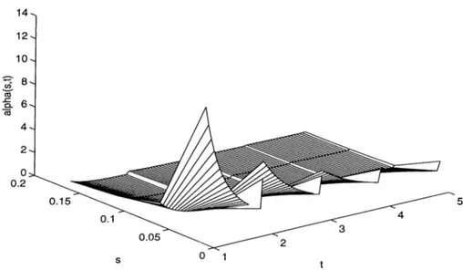
2.1 The effective bandwicltli for periodic sources. The parameters B = (/ = 1. A single unit of workload is produced at the end of every unit interval with random phase. The effective bandwidth is seen to grow over intervals shorter than the period of the source . . . . 16

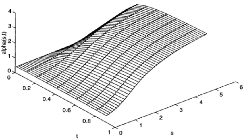
2.2 Effective bandwidth of an on /off fluid source. The parameters A = 1, /i = 9, and h = 10. The effective bandwidth approaches the mean rate Xhf{\ + /j,), as s or t approaches zero. 17

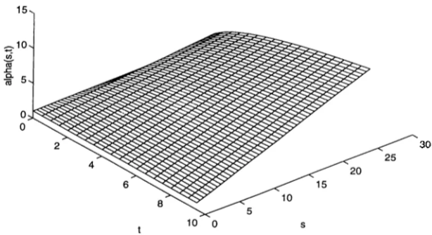
2.3 The Effective bandwidth of a Gaussian source. The parameters are H - 0.75, A = 1, and cr^ = 0.25. The long-range order is indicated by the continued growth of the effective bandwidth with large t... 18

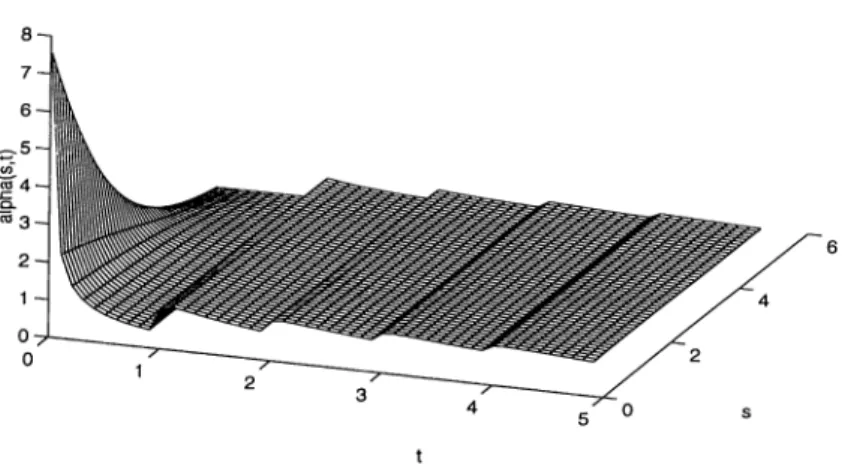
2.4 The effective bcindwidth of an O N /O FF periodic source. The pa­ rameters are p - 0.05, /? = 2, and cl = 1. The increase of the effective bandwidth as t either increases towards the interval over which the source remains ON or OFF, or decreases l^elow the pe­ riod of the source... 19

3.1 Effective Bandwidth F u n c tio n ... 36

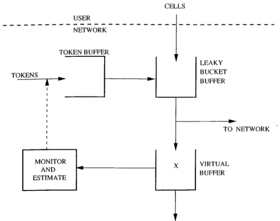
3.2 Virtual Buffer M o d e l ... 37

LIST OB' FIGURES XI

3.4 Estimate of A versus t i m e ... 39

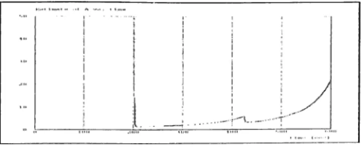
3.5 Estimate of True CLP, CLP and CLP vs. t i m e ... 40

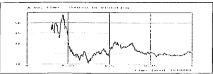
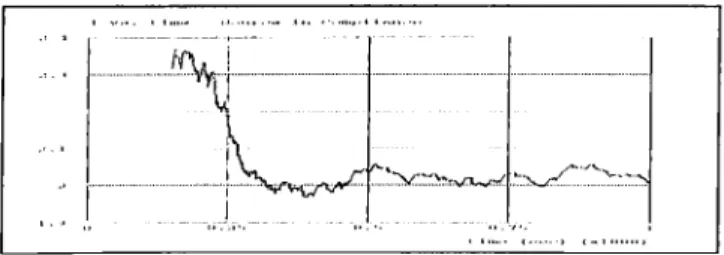
3.6 Virtual Buffer Model for Traffic Monitoring 41 3.7 Estimate of / vs. time - Source in Violation 43 3.8 Estimate of A vs. time - Source in V io la tio n ... 43

3.9 Estimate of I vs. time - Source in C om p lia n ce... 44

3.10 Estimate of A vs. time - Source in Compliance 44 3.11 Model for New Scheme 48 3.12 Modified Model for New Scheme 49 3.13 Estimate of a versus / .i... 50

3.14 Estimate of 6 versus /r 50 3.15 Estimate of p and liatp versus p, 51 3.16 Estimate of p and p vs. p - Magnified Figure ... '. 51

3.17 Estirncvte of pd and pd versus, p ... ; ... 52

4.1 Model for C A C ... 57

4.2 Model for Merging Input Streams and Pertbrming C A C ... 67

4.3 Source 1- Estimate of C W T D vs. p ... 68

4.4 Source 1- Estimate of Bcwtd vs. p ... 68

4.5 Source 2- Estimate of C LP vs. p ... 69

LIST OF FIGURES Xll

4.7 Source 3- E,stimate of CLP vs. ¡ . i... 70

4.8 Source 3- Estimate of Вф vs. /.i... 70

4.9 Source 3- Estimate of C W T D vs. /л... 71

Chapter 1

Introduction

The trend of current and recent developments in telecommunication networks is towards high-speed digital networks, notabl}^ the ATM-based B-I8DN, which are expected to support heterogeneous classes of traffic, ea,ch usually requiring a. different quality of service (QoS). This environment, though flexible enough for siq^porting existing cuid future services, presents a dynamic nature that poses complex resource management problems when trying to achieve efficient use of network resources. Efficiency and higher resource utilization are met through statistical multiplexing. The kitter, in turn, requires a complete characterization of the traffic. Hence, traffic characterization has an important role to play in the design and control of networks that would be able to cope with bursty multi- media traffic and guaranteed QoS.

Work has been done on a measure that captures the chara.cteristics of tlu? source, including its burstiness, and the service requirements. This measure is known as the effective bandwidth.

A measure of the performance of a traffic descriptor such as the effective bandwidth may be the cell loss probability (CLP) at the buffer. Hence, tlie problem of determining CLPs in queuing systems is also crucial in the develop­ ment of emergent technology of networks using A'l'M. However, as A'l'M networks

Chapter 1. Introduction

would support bursty multimedia traffic, often multiplexing a Icirge number of in­ put streams, an exact analysis cuid Ccilculation of the CLPs is intrcictable. In the presence of very small CLP values of the order of 10“ '^ and reasonably large buffer sizes, as in an ATM context, a large deviation cipproach (Appendix A) may be adopted, and the effective bandwidth acts cis an cisyrnptotic a.pproximation to the tail probabilities of loss.

To have a better view and understcinding of the effective bandwidth concept, we provide a brief overview that covers the motivations behind such a theory and the major developments that have been reached so far.

The traditional circuit-switched network assumes that each call of class j

requires cui amount of capacity ajk at link k. The capacity requirement c\jk is constant throughout the connection. The theory of such networks is rich, a.nd well-understood. However, what if ci call’s resource requirements are to vciry randorrdy over the call’s duration ?

Hui [25,26] investigated the case of a simple model of unbuffered resources. He assigned to each time-varjdng source of class j a measure of the I'eal, true bcuidwidth requirement cVj which he termed the effective bandwidth of the re­ source at each source of class j. I ’lie effective bandwidth o;./ depends on the characteristics of the source of class j such as its burstiness, and on the degree ol statistical multiplexing possible at the resource. Kelly [27] generalized the notion of the effective bandwidth to certain models of a buflered resource. This would enable to carry the insights available in the circuit-switched networks to these new emerging ATM networks.

Gibbens and Hunt [21] defined the effective bandwidth tor a unilorm arrival, uniform service (UAS) model. Its calculation is found to be quick, simple and efficient. The multi-service network reduces to a. circuit-switched network.

Guerin et al. [23] proposed a computationally simple approximation lor the effective bandwidth (also referred to as the equivalent capacity in the literature) for individual and multiplexed connections. They derived an exact computational procedure for the effective bandwidth, though intractable in an A'fM networks context.

In [5], Chcing developed a. general framework lor the theory of the effective bandwidth through the large deviation principle. He defined a caJculus lor net­ work operations based on the effective bandwidth. The importance of his work is that it nicide possible to extend the single queue results to the network case.

Chcipter 1. Introduction 3

El Walid and Mitrci [20] derived the effective bcuidwidth for general Marko­ vian traffic sources. The effective bandwidth emerged as an explicitl^^-identified and a simply-computed measure. Its computation depends only on the source characteristics and not on the system. This lead to a decentralized estimation for the measurements.

Lciter, the effective bandwidth, through a heuristic approach, was proven to exist for multiclass Markov fluids and other ATM sources (constant rate memory- less sources, discrete time Markov sources, Markov fluids and Markov-modulated Poisson processes) [29]. It was regarded cis the fixed rate at which each source is transmitting, in a small CLP context. It does not depend on the number of sources sharing the buffer nor on the model parameters of the other sources.

In [17], the effective bandwidth was defined as the minimum bandwidth re­ quired by the connection to accommodate its desired QoS. Their work intro­ duced an on-line resource management application, namely traffic monitoring, that makes use of the effective bandwidth concept.

Recently, Kelly [28] presented a synthesis work on the effective bandwidth theory. He stressed the unifying role of the concept, as a summary of the statisti­ cal characteristics of sources ovcir time and space, as a limit and an approximation lor models of multiplexing under QoS constraints and as a basis lor simple and ro­ bust scheme for resource management applications such as connection admission control (CAC) mechanisms for a poorly characterized traffic.

It is important to note that, while the effective bandwidth theory is well- defined and understood, very few attempts have been made so as to clea.r tin; way to a functional use of it. An application of the theoretical tool to the real world problems is essential. Our main concern, in this work, is to investigate procedures that ma,ke use of the effective bandwidth concept for on-line, real­ time resource maiicigement in ATM networks. Moreover, the effective bandwidth

Chcipter 1. Introduction

analysis is generally addressed on a single source model basis. However, resource mancigernent in ATM networks is not oi^timal unless stci.tistica.1 multiplexing is exploited cind the gains ixchieved therein are accounted for. Hence, merging in­ put strecims together on a single link and performing network applications on a rnultii^lcxed basis is especially of concern.

Our work is organized as follows. Chapter 2 is devoted to a detailed literature review of the effective bcindwidth concept. We cover the theory of the effective bandwidth along with some illustrative examples, introduce several traffic de­ scriptors and examine the major resource rnanagement applications. Chapter 3

describes and simulates two schemes for on-line, real-time, ATM source charac­ terization. Specifically, based on a model suggested by De Veciana et al. [17], we estinicite, via on-line measurement, the performance of a source. An applica­ tion of this estimation procedure, namely traffic monitoring, is illustrated for a Markovian arrival process. The second scheme, suggested by Mark et al. [32], enables characterization of general types of sources with no restrictive assump­ tions on the type of offered traffic load. This methodology is also studied and its improved features over the former are emphasized. Once sources are charcxcter- ized, resource management issues can be addressed in either of two ways: Sources may be either treated individually or on a multiplexed basis. In Cliapter -4 we present our work for the multi-source case. We focus on CAC using both the in­ dividual and the multiplexed cvpproaches. Since efficiency and optimal utilization of network resources cire met through stcitisticcd multiplexing, our work focuses on merging severed iniDut streams together on a single link and account for the gains achieved therein. Based On this new approach, we suggest a novel, optimal CAC scheme. Owing to the inherent shortcomings of the effective bandwidth concept. Chapter 5 sumnicirizes the major limitations and criticism addressed to this approximation and stcites our concluding remarks.

Chapter 2

Effective Bandwidth: Review, Theory and

Applications

2.1

M ajor Works on Subject

We present a detailed literature review that covers the niotiva.tioiis behind the eifective bandwidth theory, its aims, the major developments that have been reached so far and their underlying limitations.

As mentioned in the Introduction, the traditional circuit-switched network assumes that each link k has a. capacity 6\· and that each call of class j requires an amount of capacity aj^ at link k. The network is able to carry rij calls of class

j if Tijajk < Ck- The theory of such networks is rich and well-understood. However, what if a call’s resource requirements are to vary randondy over the calls duration ?

Hui [25,26], for a simple model of unbuffered resources and using the large deviation approximation (Appendix A), showed that the probability of resource overload can be held below a desired level by imposing that tire number of calls

Chapter 2. Effective Bandwidth: Review, Theory and Applications

rij acceiptecl from sources of class j satisfies

(

2

1

where C is the capacity of the resource and aj is the effective l)andwidth of the resource at each source of class j. 'f’he effective Ijandwidth a./ depends on the characteristics of the source of class j such as its burstiness and on the degree of statistical multii^lexing possible at the resource. The obtained results were asymptotically exact.

Kelly [27] generalized the notion of the effective bandwidth, additive over sources of different classes, to certain models of a buffered resource, introducing finite size buffers is important for they disable traffic fluctuations for the streams sharing the resources. Most importantly, this would enable to carry the insights available in the circuit-switched networks to these new emerging ATM networks. The models considered were the M /G /1 and the 6 ///C //1 queues. Kelly concluded that this concept is important for source classification and admission control. The major drawback is in overload, i.e., for large resource capacity C and larger effective offered load, the accepted sources would be l^iased towa.rds tliose with low effective bandwidth.

In [21], Gibbens and Hunt defined the effective bandwidth tor the uniform arrival, uniform service (HAS) model. They considered heterogeneous O N /O F F sources which alternate between exponentially distributed periods of transmission at the peak rate and idleness. The effective bandwidth is found to be a measure that depends only on the mean bandwidth, burstiness of the source and the channel. Its calculation is found to be quick and efficient. The multi-service network reduces to a circuit-switched network.

The work found in [21] was based on [2]. Therein, the authors analyzed the statistical multiplexing of N sources of a single type onto a communication channel. So, two generalizations had to be investigated: (i) Case of more than one single channel type, and (ii) case of a network of such channels, d'o investigate the first issue, one could think of solving a set of single-type source problems. However, this turned out to be wrong. Instead, lor m different types of sources.

Chapter 2. Effective Bandwidth: Review, Theory and Applications

an efFective bandwidth is defined ci,s the set

i^ ,p ) = {N = (Ni,N2,..N„,,) : Pat (queue length > B) < p}, (2.2) Q'

wliere B is tlie buffer size and p is the cell loss probability (CLP). For p of the order of 10“ ^, the large deviations approach is used and a {B ,p ) is approximated by

a{B,p) = {N = (M,iV2,..fV„0 : Y^mcxi < C}, (2.3)

i

where cv; is the effective bandwidth of type-« source. This approximation would make it possible to analyze the two issues cited above. Specifically, the author distinguished two cases. For large buffer size B, log{p)lB tends to G [—oo,0],

approximation (2.3) Wcis shown to be exact, and for an O N /O F F type-i source with ON and OFF periods exponentially distributed with means and

« ¿ (0

_ i n + hi + Ai - + Pi - A,:)2 + 4A,:|tt,:

2^

(2.4)

where 7; is the constant rate of transmission of source of type i while in ON state.

Note that, = 0 corresponds to

K li

a¿(

0

A; + 7i

That is, the effective bandwidth is taken as the mean rate, which is a lower bound. The only constraint on the system is that it be stable. This is due to the long time elapsed before the buffer size is exceeded, and sources have bcien tlirough their ON and OFF periods many times. The other case is For ^ = —00. Then,

cvi(-oo) = 7i. (

2

6

This corresponds to the peak rate. This happens when the source is so l)ursty, that a peak rate bcuidwidth allocation is needed. Hence, the measure C = f —

I _ Ç [0,1] is the asymptotic system burstiness, i.e., the larger C, becomes the more susceptible the channel is to burstiness. The fact that ( depends on the channel only, and not on the offered load, is of prime importcuice in the design of ATM networks.

Chapter 2. Effective Bandwidth: Review, Theory and Applicaiions

Рог small buffer size B, the buffer overflows if

^ > c. (2.7)

The rare event is no longer that the queue has built up, but rather that an unusually large number of sources are ON at once. For В = 0, the exact acceptance set is given by the Bernoulli model, and the UAS model turns out more accurate than the large deviation approximation. For В small, but non­ zero, the difference between the two approximations is large, l^ut gets smaller as

В is increased. As a conclusion, the effective bandwidth is valid lor finite buffer size B, with different levels of accuracy.

Guerin et al. [23] proposed a computationally simple approximation for the effective bandwidth (also referred to as the equivalent capacity in the literature) lor individual and multiplexed connections. This unified metric would turn out to be useful for bandwidth management, routing and call control procedures. It should be emphasized that their methodology can provide an exact со т р и tationa.1

procedure for the effective bandwidth, but its complexity makes it intractable in real-time network traffic applications. Thus, an approximation is more appropri­ ate. The first approximation is based on the fluid-flow model (continuous-time Markov chain) and the second is the stationary approximation for the bit rate distribution. In most cases where the statistical multiplexing effect is significant, the distribution of the stationary bit rate can be accurately approximated by the Gaussian distribution. However it should be emphasized that the second approximation does not hold in the case of sources with long burst periods (as for the asymptotic approximation on the large buffer size). The authors argued that even an exact model does not provide a correct measure of tlie GLP seen bj^ connections, as it is unable to fully capture the impact of the interactions within the network.

In [4], Chang developed a general framework for the theory of the eflective liandwidth. A general form of the effective bandwidth was derived using the large deviation theorem. The following calculus for network operations was found: (i) 'file effective bandwidth of multiplexed independent sources is less than the sum of the effective bandwidths of the sources, (ii) the distribution ol delays a.nd

Chapter 2. EíFective Bandwidth: Review, Theory and Applications

queue lengths is bounded by exponential tails if the effective bandwidth is less than the channel capacity, (iii) the effective bcuidwidth of the output is less than the effective bandwidth of the input, (iv) the effective bandwidtli of a routed process from a departure process can be derived from tlie effectives l:)a.ndwidth of the departure process cind the effective biindwidth of the routed process. The importance of these rules is that they make possible to extend the single queue results to the network Ccise.

In [5], an intuitive derivation for the effective bandwidth was given. To achieve this goal, and instead of investigating the queue behavior at the packet level, time and space were scaled, yielding the approximation of ATM networks by stochastic fluid network, with external inputs given by the Gibbs distribution. The tail distribution of queue lengths in fluid networks could then be solved by simple minimization problems.

El Walid and Mitra [20] derived the effective bandwidth for general Markovian traffic sources, with no restrictions on their dimensionality, homogeneity or time reversibility. They defined the effective bandwidth as the maximal real eigenvalue of a matrix directly olitained from the source parameters and the admission criterion (network resources and service requirements).

The source is characterized by (M , A), where M is the irreducible infinitesimal generator of a Markov chain arid is the source constant rate at state s.^ Let

G {B) be the stationary P r { X > B), where X is the random buffer content and

G{B) the overflow probability for a buffer of size B. The admission criterion is

G{B) < p. The asymptotic regime states that p tends to 0 and B tcnids to infinity. In this case log(p/i?) tends to ^ E [—oo,0j. fl'lie effective Irandwidth depends on (M, A) , and on the l^nffer and overflow ])rol3ability oidy tlirouglt The effective bandwidth a turned out to l)e the maximal real eigenvalue of the matrix

A - (

2

8

where A = diag{\). For A; sources characterized by A*^'^), cv =

Chcipter 2. Effective Bandwidth: Review, Theory ¿ind Applications ₁₀

eigenvalue of the matrix,

i A ^

1 - e^'

tM (2.9)

Hence, the effective bandwidth is an explicitly-identified, a simply-computed measure. Its computation depends only on the source characteristics, and not the system, which leads the wa.y to a decentrcdized estimation lor the measure­ ments. It has correct properties at the natural cisyrnptotic regime (CLP tends to zero and buffer size tends to infinity) of the small loss probabilities. The authors considered both Markov-modulated fluid and point processes (such a.s Mcirkov- modulated Poisson or phase renewal processes). Most importantly, the effective bandwidth notion acts as a bridge to the familiar circuit-switched network de­ sign. Numerically, the effective bandwidth provides a. conservative bound on the acceptance region, and contrary to the mean and peak rates, it jrrovides an ef­ fective basis for admission control. Finally, in the presence of a leaky bucket, the effective bcindwidth decreases, by time, from the maximal effective bandwidth of the source to a lower value.

Later, the effective bandwidth, through a heuristic approach, was proven to exist for multiclass Markov fluids and other ATM sources (constant-rate memory- less sources, discrete-time Markov sources, Markov fluids citid Markov-modulated Poisson processes) [29]. It was regarded as the fixed rate at which eacli source is transmitting, in a small CLP context. It does not depend on the number of sources shciring the buffer nor on the model parameters of tlie other sources. Again, the buffer size was assumed infinite and the source was subject to the same assumptions cis in [5].

Gun et al. [24] investigated the effective bcindwidth vectors for multiclass traffic multiplexed on a partitioned buffer. Their model included a single source generating j different classes of traffic and Vcu'ious independent, lieterogeneous and Markov-modulated fluid sources multiplexed into a single buffer. They de­ fined an effective bandwidth vector corresponding to the j (JoS classes. In tlic;ir analysis, they used the property that if the sum of the effective bandwidth of all the sources multiplexed onto the buffer is less than the speed ol the channel to remove the data from that buffer, then the QoS is satisfied lor all the sources.

CImpter 2. Effective Bandwidth: Review, Theory ¿md Applica tions ₁₁

Moreover, this work is valid lor sources with close QoS requirements. In practice, when sources have different QoS, they all line up to the stringent QoS. This re­ sults in sub-optirnal resource allocation. The solution can be to classify traffic into multiple classes according to their QoS and to assign a separate buffer for each. However, this method has many drawbacks. It is better to adopt a slianed buffer scheme. Yet, the effective bandwidth approximation is again based on the large buffer asymptotics. This can significantly overestimate (in the case of sources that are more bursty than Poisson) or underestimate (in the case of sources less bursty than Poisson) the number of sources that can be multiplexed on a trunk. The effective bandwidth vector is not additive, provides an approximation and not a bound and leads, numerically, to sub-optinicil buffer thresholds.

In [17], the effective bcindwidth was defined cis the minimum bandwidth re­ quired by a connection to accommodate its desired QoS. Based on huge devia­ tions, an effective bandwidth approximation was found to mimic the tail probabil­ ities of loss. For cl. buffered link with capacity c cells/sec, supporting a. stationary and ergodic cirrival packet stream /1(0, ¿), let X be the buffer’s stationary work­

load. QoS aims to limit the likelihood of large delays or to ensure that CLP is small. Based on the large deviation theorem, the tail probability of loss is approximated by

F { X > B) < p = < 1, (2.f0)

where h is a measure of the stringency of the QoS requirement and B is the buffer size. The effective bandwidth function is defined b}^

cv(^) = S ' liin t

¿—>■00

- 1

log

(

2

.

11

)

The derivation is as follows. Under mild conditions for both continuous and discrete-time arrival processes, and for all <5 > 0,

cv(6) < c lirn B~^ log [P{ X > B)] < - 8, B-^oo or equivalently. P { X > B ) = exp - B a - T c ) + oiB) (

2

12

It was used as a traffic descriptor for traffic monitoring, d'he traffic con­ sidered was one that tolerates statistical QoS guarantees, and again tlie large

Chcipter 2. Effective Bandwidth: Review, Theory and Appiiccdions ₁₂

deviation assumptions were made. On its viability as a traffic descriptor, it turned out to be efficient, reasonably accurate, robust and simple in the sense of implementation and performance. On its accuracy a.nd the rela,xation of the stationarity assumptions, it turned out not to capture all the statistical multi­ plexing gains. One way to solve this is to use refined asymptotics [9] (Section 2.3.1), or to combine the effective bandwidth with a zero-buffer approximation. As for the quasi-static approximation (the assumption that the system reaches steady state), it could not be relaxed. The effective bandwidth approximation is:

P ( X > B) ^ Aexp{—BI ) RS exp{—BI), where I = q“ ' (c). Thus A is approxi­ mated as 1. However, in reality A may be large, or small. Determining A may be prohibitive and would make bandwidth mcuiagement leased on the effective Ijandwidth inefficient. A remedy to this would be to measui-e the extent of the statistical multiplexing gciin (A) cuid change the admission criterion (é) [30]. But, this solution requires a complete specification of the entire effective bandwidth char cicteris tics.

In [15], the effective bandwidth was derived for stationary sources. It has been computed as a function ol the mean ixite, index of dispersion and the bulfer size. Specifically, for a stationary process Xn with kth order autocovariance j { k ) cUid spectral density function f{u>) = 7(A.·) exp(fa;A:), the index of dispersion

7 is defined as

CO

7 = 7t/( 0 ) = Y2 7(^·)· A:= —oo

The assumption is that the process should be purely indeterministic without periodicity or long-term dependencies. As for the effective bandwidth and for Ni

stationary, independent inputs satisfying the Gartner-Ellis theorem (Appendix B), each with mean pi cuid index of dispersion 7;, the effective bandwidth rv,: associated with each source is

h i

9

— hi + + <'-^(^)î (2.f5)

where 8 is a measure of the stringency of the QoS requirements. Moreover, formulae for Markov-modulated fluid (two-state fluid, M /M /00, //.-state fluid) were also given therein. These forrnulcie have been tested numerically in [16] and yielded good results.

Chcipter 2. Effective Bandwidth: Review, Theory and Applications 13

A simple, intuitive overview on the effective bandwiclth theory was presented in [4]. The approcich was through the large deviation theory and the Laplace method of integration. It includes: (i) Identification of the energy function, en­ tropy function and the effective bandwidth function, (ii) a calculus of the effective bandwidth function, (iii) bandwidth allocation and buffer management, (iv) traf­ fic descriptors cind (v) envelope processes and conjugate processes, a method for fast simulations and bounds. The effective bandwidth is regarded as the min­ imum bandwidth to satisfy the corresponding QoS. fo r a source modeled as a constant-riite fluid with rate Л on a period of time t and probability density func­ tion /(A ,Z ), the tail distribution of the queue is given by the integral of /( A ,/) . Using the large deviation theorem, /ÏA, t) is shown to ha.ve the Gibbs distribution, i.e.,

f{ X, t) = exp(-fA *(A )). (2.16)

A*(A) is the energy function obtained from the Legendre trciiistbrmation of A(d), i.e..

A*(A) = sup(dA — A(d)), (2.17)

and A(fl)is the entropy function obtained from the Gartner-El lis limit of a source,

1 r

A(d) = lirn - log .

i-i-oo i L (2.18)

Then,

„ . (0) = _(2.19)

is the effective bandwidth function. Note that c\*{0) is increcising in 0, it tends to the average rate as 0 tends to 0 and tends to the peak rate as 0 tends to infinity. The calculus of the effective bcindwidth is then derived heuristically. It mainly shows that the effective bandwidth of multiplexing independent arrivcds is additive. As for the application of the theory to networks, tlie results are asymptotic, in the sense that they yield very loose bounds for finite l)ufler sizes. 'I'lie independent input assumption makes it difficult to analyze networks with loops.

Chapter 2. Eilective Bcindwidth: Review, Theory and Applications 14

l.heory. He stressed the unifying role of the concept, as a sumniary of the statisti­ cal characteristics of sources over time cincl space, as a limit and an approximation for models of multiplexing under QoS constraints a.nd as a l)asis for simple and ro- l)ust scheme lor tariffing and connection admission control mechanisms lor poorly characterized trciffic. The material found in the next section is inspired mainly from this work [28].

2.2

Effective Bandwidth Theory

In what follows, an alternative definition of the effective bandwidth is given, along with some of its major properties and examples. Later, the theory is ext(Mided to some common multiplexing models. Note that the effective bandwidth, defined next, is associated with stationary sources.

2.2.1

Definition

Kelly [28] defines the effective bandwidth in terms of two free parameters, .s· and /., representing the space and time scales, respectively. The appropriate choice of .s and t will depend on the chai’cicteristics of the resource (capacit.y, buffer size, traffic mix, scheduling policy, etc.).

Let A"[0, /] be the cunount of work arriving from a source over a time inter­ val [0, /] and let X [0,t] have stationary increments. The effective bandwidth is defined cis

a{ s, l ) = i log

st (

2

20

2.2.2

Properties

1. If .^[0, /] hcis independent increments, then (y{s, t) does not depend on t.

2. ifX [(), i] = XZ for i > 0, then cv(s, ¿) = o-fs/, 1), i.e., cv(s,/) depends on

s and t through the product st only. Otherwise, a{s/t, t) is strictly decreasing in

t.

3. Additive Property - If A"[0,Z] = I]; A",[0,Z], where (^¿[O,/]),· are indepen­ dent, then

a{s,t) = ^ cv,:(s,Z ). (2.21)

Chapter 2. Effective Bandwidth: Review, Theory and Applications 15

4. For any fixed value of ais. t) is iricrecising in .s, and lies between the mecui and the peak of the arrival rate rnecisured over an interval of length /, i.e.,

m

A <

< A M

₂

₂₂

2.2.3

Examples

'lb have a better appreciation of the effective bandwidth concept, Kelly [28] de­ rived some closed form expressions for some common source tyjres. 'I'hese are presented here along with some illustrative figures.

Periodic Sources

'I’liis model can be used to describe arrivals of constant-ra.te sources. Let B units of workload be produced at times Ud nd, n = 0,1, . . . , where / / is unitorndy distributed on the interval [0,1]. The effective bandwidtli function is given by

/ X B pt , 1 , a ( s ,0 = J [~i\ + -_st log

Note that

limcv(s,i) =

Î- . 0

An illustration of Eqn. (2.23) is given in Fig. 2.

( t - - n j . (2.23)

c » ‘ - 1

ds ■ (2.24)

Chapter 2. Effective Bandwidth: Review, Theory and Applications ₁₆

Figure 2.1: The effective bandwidth for periodic sources. The pcirarneters B - d = 1. A single unit of workload is produced at the end of every unit intervcil with random phase. The effective bandwidth is seen to grow over intervals shorter than the period of the source

Fluid Sources

Let a stationary fluid source be described by a two-state Markov chain. The transition rate from state 1 to state 2 is A and the transition rate from state,2 to state 1 IS p. While in state 1, workload is produced at a constant rate /?,, and no workload is produced at state 2. The effective bandwidth function is given by

/ exp

1

\\ma{s,t) = - (hs - p - X + J( hs - p + A)^ + ipX). (2.26)

In general, lor a stationary source described by a finite Markov chain with stationary distribution tt and q-matrix Q, with the workload produced at rate hi

while in state i,

(2.27)

1

Chapter 2. Effective Bandwidth: Review, Theory and Applications ₁₇

where h = diag{hi)i.

Note that

1

^hmo;(5,Z) == ^ (/){s), (2.28)

where (j){s) is the largest real eigenvalue of the matrix Q + hs. An illustrcition of Eqn. (2.25) is given in Fig. 2.2.

Figure 2.2: Effective bandwidth of an on /off fluid source. 'The parameters A = 1,

p = 9, and li - 10. The effective bandwidth approaches the mean raté A/?,/(A+/i), as s or t approaches zero.

Gaussian Sources

Consider X [0 ,i] = Xt + Z[t), where Z{t) is normally distributed with zero mean, then,

(2.29)

a{s,t) = A + — Var[Z{t)].

In the heavy traffic case, Var[Z(t)] =

In general, Z is a fractional Brownian motion with Hurst parameter H E

(0,1), and Var[Z{t)] = . Then,

Chcipter 2. Effective Bandwidth: Review, Theory and Applications ₁₈

If H < 1/2, limt_oo « (s , i) is finite and does not depend on .s; if H —1/2,

limt-,ooCi{s, t) is finite but depends on s; and if H > 1/2, a(s, t) grows as a fractional power of t. The latter case exhibits long range order. An illusti’cition of Eqn. (2..30) is given in Fig. 2.3.

30

Figure 2.3: The Fffective bandwidth of a Gaussian source. The parameters are

II = 0.75, A = 1, and = 0.25. The long-range order is indicated by the continued growth of the effective bandwidth with large t.

General O N /O F F Sources

The source in this case alternates between long periods in ON state with effective bandwidth a i(s , t), and long periods in OFF' state where it produces no workload. Let p be the proportion of time spent in the ON state. For values of t small compared to periods spent in ON and OP'F states, the effective bandwidth is

4 log[l + p (ex p (siai(s, ^)) - 1)],

st (2.31)

where cvi(s',i) is given by (2.23). An illusti'cition of Fqn. (2.31) is given in F'ig. 2.4.

Chapter 2. Effective Bandwidth: Review, Theory and Applications ₁₉

Figure 2.4: The effective bandwidth of an O N /O F F periodic source. The param­ eters are p = 0.05, B = 2, and d = 1. The increase of the effective bandwidth ivs t either increases towards the interval over which the source remains ON or OFF, or decreases below the period of the source.

2.2.4

Multiplexing Models

Owing to the importance of multiplexing in achieving efficiency and optimal­ ity in resource management in ATM networks, Kelly [28] suggests the following multiplexing scheme.

Let the arrival process be as follows:

A'[0,i] = E E A id O .i], j = l i=l

(2.32)

where iXji[0, t])ji are independent processes with stationary increments whose distribution may depend on j , but not on i. Let there be a resource to cope with the ciggregate arriving stream, iij is the number of sources ol type j and Cij(s, t)

is the effective bandwidth of a source of type j. Hence,

Chapter 2. Effective Bandwidth: Review, Theory and Applications ₂₀

For several multiplexing models to come, we would be interested in the rela­ tionship between the constraint

^ n , a , { s \ n < C*, j=i

(2.34)

lor choices of and the cicceptance region defined as the set of vectors

(ni,n2, ■■■P'lj) lor which a given performance, in terms of queuing delay or buffer

overflow, is guaranteed. Bufferless Models Let J nj = E E E . . j = l i= l (2.35)

where Xji are independent random variables with scaled logarithmic moment generciting functions

(2.36)

aj{s) = - log

Xji may be regarded as the instantaneous arrival load at a bulferlcss resource of Ccipacity C, so that Cij{s) = linii_,o cvj(.s/Z, i). Chernoff’s bound yields

log7^(A ^>60 < log = sicxis) - C), (2.37)

where cv(.s) = ^y?rjCVj(s). Hence, \ogP{X > C) < —7 is satisfied within the set.

A = \n ■_^ . inf

O 5 - C) < —7} for n > 0. (2.38)

The half space touching at a point n* on the boundary ot region A is

Chcipter 2. Effective Bandwidth: Review, Theory ¿ind Applications 21

where s* scitisfies the iniimum in (2.38) with n replaced by n*. This is a conserva­ tive bound on the non-linear acceptance region for a bufferless model. Applying the Chernoff theorem, we get

A i j N , CN)

lim

N-^OO N = A·, (2.40)

that is, as the number of sources increases and the tail probability decreases, the approximation made to lead to the region A becomes more accurate.

M /G /1 Models

In this section, (2.34) will emerge as the linear limiting form, conservcitive bound, on the acceptance region for a buffered model with general input processes.

Let Xji[td,t] have independent increments, ctj{s) = a.j(s, t) and «(.s) = c\{s,t).

Let Q he the stationary workload in the queue and C the capacity of the server. The buffer size is infinite. The Pollaczek-Khinchin formula is

C - cv(0)

C - a ( s ) ‘ (2.41)

Let K be a finite constant such that cv(«;) = C , then the Cramer’s estimate gi ves

C — cv(0) .¡^ P{Q > B)

K a [k] as B ^ GO.

F’or P(Q > B) < —7, n e .4(7 , B), Cramer’s estimate implies

lim A (7AI , BN) - A, N—yoo where A = {n : Y^rij a { ^ ) < C}. (2.42) (2.43) (2.44)

So far, we were concerned with the proportion of time the bufter occupancy e.xceeded a level B in a queue with cin infinite buffer. Next, we will consider the case of a finite buffer size where the workload exceeding this level would be lost.

Chapter 2. EfFective Bandwidth: Review, Theory and Applications 22

Finite Buffers

IxM, the proportion of the workload lost in the finite buffer be L{B). From (2.42), we deduce

L{B) --- C {C - a { h ) f as B ^ o o .

K, a ( K,) cv(Uj (2.45)

For log L{B) < - 7, n e Apropic^

lirn A i'iN , BN) = A.

N—+00 (2.46)

Mean Delays

From the Pollaczek-Khinchin formula (2.41), it follows that EQ

and the constraint EQ < L is satisfied if and only if

J2L

i=l + - H—

<

c.

(O' - cv(0))

(2.47)

Buffer Asymptotic Models

For models more general than the MIG/l, tciil probabilities decay exponentially. To see this, consider an arrival stream A [0,f] with stationary and ergodic incre­ ments. Let Q be the stationary-distributed worklocid of a queue with capacity C

and finite buffer size B. Let

limcv(.s,i) = a:(s). t—^OO

(2.48)

Let there be a finite constant k such that Q'(«) = C and a (k) is finite. Then,

Jim i log PiQ > B) = -K.

B-^oo Jt)

Chapter 2. Effective Bandwidth: Review, Theory and Applications ₂₃

Deterministic Multiplexing

For a server of capacity C and a buffer of finite capacity B, the condition under which the buffer capacity is never exceeded is that ri € A, where

A

_n

0 < i< o o

is the intersection of the linearly constrciined regions

B

A = < C + y } ·

(2.50)

(2.51)

2.3

Applications of Effective Bandwidth Theory

As the effective bandwidth formulation is rcither siniple and robust, the theory has niciny applications in high-speed digital networks, such as ATM. The main applications we will encounter in this section are the ones dealing with resource maimgernent in ATM networks. Resource management is an important issue in the design and implementation of such networks, for it lea.ds Uie way to achieve optimality in their use, maximize their efFiciency, enhance their reliability and thus ensure their viability.

2.3.1

Effective Bandwidth as Traffic Descriptor

'lb derive the bandwidth requirement of a service, one needs to characterize its traffic pcittern, either by a set of traffic descriptors or by a matfiematical inodef. 'I’he latter is known to be intractable in an A'FM networks context, 'rraffic descriptors, such cis the effective bandwidth, can be used to approximate the given traffic. 'I'he (JoS can be formulated in terms ol the (JLP in tlie queue, i.e., for a. traffic workload X and a buffer capacity B, tfie CLP is B{X > B),

or in terms of the deiay experienced by the packets (or cells) in the queue, that is, P { W > t) for W being the waiting time. Clearly, these two measures of performance are related. In what follows, we present tfie main traffic desci-iptors.

Clmpter 2. Effective Bandwidth: Review, Theory and Applications 24

Three-parameter Approach

In (Juerin et ai. [23], traffic was characterized by three parameters: peak rate Ap, avei'cige burst period b cirid the utilization p (i.e., fraction of time tlie source is active). These parameters were then mapped to an O N /O F F Markov fluid (fluid-flow approximation). For a finite buffer size D, the equivalent capacity (effective bcuidwidth), cv, is related to the overflow probability p by

p = ^ exp - B{a - pXp) where /9 is ^ -6(1 - p)(Xp - cv)cv/’ (a - pXp) 4- ppjXp - a) (1 - p)a (2.52) (2.53)

Typically, ff is taken as 1. For the single source case, the eiiuivalent ca.|)a.city is given as

( l / p )6(l - p)Xp - B + ^ [ ( l / p )6(l - p)Xp - BY + 4B{l/p)bp{l - p)Xp a —

2( l / p )6(l - p)

(2.54)

Extending the result to the multiple source case, the equivalent’ capacity is simply

,c v = (2.55)

where cxi are determined from (2.54).

Note that for connections with long burst periods and low utilization, /9 is significantly different from 1. However, multiplexing a numl)er of connections with long burst periods can be approximated by a stationary bit rate distribution (stationary approximation). The equivalent capacity (A is given by

Cs = rn + pa, (2.56)

with

Chciptcr 2. Effective Bandwidth: Review, Theory and Applications 25

where m is the mean aggregate bit rate (771 = ?'«;) aiKl a is tlu; standa.rd

deviation of the aggregate bit rate (cr^ = erf)·

Combining the two approximcitions, the equivalent capacity C is simply the minimum between Cp and Cs, namely

N

C = rnin(??2 + p (7 , 6V,·). i=l

(2.58)

Four-parameter Approach

In [5], a four-parameter trafhe descriptor is obtained. These four paicuneters are relcited to the iiverage rate, ¿isymptotic variance, peak rate and average burst duration of the source. The derivation is ¿rs follows: the effective bandwidth function may be expanded at = 0 and 0 — 0 0 to give

cy*(0') — 1]i T fj2^ T ^ ^ d,

= 7]3 '1^ ^ i ^ \ /)

j + " 00,

(2.59)

(2.60)

where rp is civerage rate, 2rj2 is the asymptotic variance, r/3 is the peak rate and

7/4 is the average burst period.

Let /( c ) be the inverse function of the effective bandwidth function (T{0), 0 — /( c ) is the solution of a*i0) — c. 1(c) has a zero at 7/1 and a pole at 7/3. Hence, c - 7/1 /( c ) (c - i/3 )(^ c + fh)' where and

1

So, the queue length distribution can be approximated l)y

Clmpter 2. Effective Bandwidth: Review, Theory ¿ind Applications 26

'rhe model considered assumes infinite buíTer size cit each queue, and to apply tlic large deviation theorem, the source is assumed to he; jointly stationary and ergodic, among other assumptions so as to satisfy the Cartner-Ellis theorem. It should be pointed out that the latter theorem is valid for finite dimensional random vectors instead of stoclmstic processes; moreover, the large deviation principle is only valid for independent, identically distributed random variables. The numerical results therein show that the effective bandwidth approximation holds for the case of positively correlated sources and negatively correlated ones. It is worth pointing out that these parameters //¿’s and especicdly the asymptotic variance /72 are hard to measure in real life applications.

First Order Exponent

The effective bcindwidth is the traffic descriptor of predilection in our work. Recall from Eqn. (2.11) that the effective bandwidth function as proposed by De Veciana et al. [17] is as follows. For a statioiiciry and ergodic arrival stream /1(0, t) and a stationary workload X , the effective bandwidth has been approximated by

cv(¿) — 6 ^ hrn t Vlog [E’ {exp [ó/l(0, /)])]. (2.65)

In considerable generality, the cell loss tail probabilities are asymptotically exponential, i.e., for a buffer workload X and finite buffer size B

P i X > B) « fte-'’® a,s B 00,

(

.

)

where a is a positive constcint called the cisymptotic constant, and h is a positive constant termed the asymptotic decay rate. The effective ba.ndwidth approxima­ tion assumes a —1.

Here, the QoS-constraint matches the CLP to the first order, that is, in tlie exponent. Recall from Section 2.1 that this result has been obtained using the asy mp tot i c cipproxi mati on.

Chcipter 2. Effective Bandwidth: Review, Theory and Applications ₂₇

Refined Asymptotics

A refined three-term approxiiricition is given in [9]. It 1ms the form

P { W > x) = -h + «3^"''^^'^ (2.67)

wliere «1 and bi are the cisyrnptotic constant and asymptotic tlecay rate as given by (2.66), while CL'i, ci:i, 62 and 63 are chosen to match the probability of delay

F ( W > 0), and the first moments EW, E(W'^) and E{W''’), with 62 and 63

required to satisfy 61 < min(62,^3)·

2.3.2

Bandwidth Management

One of the major appliccitions of the effective liandwidth theory is liandwidth allocation. Bandwidth allocation and management falls in two major categories: (i) Independent and (ii) dynamic bandwidth allocation [4].

Independent Bandwidth Allocation

Let {c(/,)}, t > 0, be an independent arrival process, so {c(/.)} is called an inde­ pendent liandwidth allocation sequence. Consider cui arrival process «(/,) with an energy function Aa{0), so

Pr{q(oo) > :c) Rs e"

if 0* is the unique solution of

Aa(f^) + Ac{ — 0) — 0.

(2.68)

(2.69)

Let A*(cv) be the entropy function of c{t) and be the global minimum of A*(cv), i.e., A*(tt°) = 0. The best bandwidth allocation is il the constant-rate bandwidth allocation sequence c{t) — a “ . In view ol the Legendre translormation.

Chapter 2. Effective Bandwidth: Review, Theory and AppHcaiions 28

the hist two equations yield

a ‘(r ) = _{< « . +} a: (cv“ ) = O'_{C 5} (2.71)

0* - " ' 0*

where cy*{0*) is the effective bandwidth function. Since it is increasing, a larger decay rate is met if the constant-rate bandwidth allocation sequence c(l.) = a)!. Hence, the optimal independent bandwidth allocation sequences are the constant- rate sequences.

Dynamic Bandwidth Allocation

Let the above defined sequence {c(i)} depend on the arrival process. Specifically, let /¿(q) for 0 < 7 < 1 be a dynamic bandwidth allocation sequence with l)eing the amount of bandwidth allocated when the l^uff'er occupancy is q.r. Since the optimal independent bandwidth allocation sequences are the constant-rate sequences, adding randomness to /¿(q) does not improve the performance of the tail distribution of the queue length. Hence, ^ti(q) can be taken as a deterministic function.

Let /i(q) be a piecewise linear function with /.¿(q) = C| for q < qj , and = 02 for q > qj . Let the arrival process a(t) have the energy function A„(tl),

the entropy function A* (a) and the effective bandwidth function For the buffer to exceed x at time t, the buffer should exceed qt.r at some time ij < t.

It then takes t — tti to build up another (1 — qi);c cells. Ihmce, tlu; problem can l)e separated to two parts: (i) The buffer to build up -y\x cells with capacity rq, (ii) the buffer to build up (1 — ■ji)x cells with capacity c^. Only when these two events happen, the buffer exceeds x. Hence,

(2.72)

where 0^ are the unique solutions of a*{0) = cq. In general,

Pr(q{oo) > a;) ~ ^ (2.73)

where 0* is the unique solution of Ci*(0) = /i(q). Hence, the eflective bandwidth for this problem is a*iO), where

0 = f'oZdj. (2.74)

Jo Pr{q{oo) P x) ~ e

Chapter 2. Effective Bandwidth: Review, Theory and Applications ₂₉

2.3.3

Admission Control

Admission control is an important issue to be considered, its main advantages are: (i) Prevention of network congestion, (ii) limiting calls and hence, guaran­ teeing a QoS.

The sources to share the resources are time-varying. Using the effective band­ width approximation, they would be regarded as constant-rate sources with the rate being their effective bcindwidth. So, the network layer and the higher lay­ ers need not be changed and this minimizes the impact of the new high-speed networks on the existing ones, such cis the circuit-switching networks.

There have been some schemes proposed for coniKiction acceptance control and we will focus on the most important ones.

Using Effective Load

Connection acceptance control is primarily concerned with expectation of the future QoS. In [28], an effective and robust use of prior declarations and empirical averages is made. The key idea was to use the prior declarations to choose a linear function that bounds the effective bandwidth function. Once this is done, the connection acceptcince control would be based on relatively simple measurements needed to evaluate this function. Specifically, let

(2.75)

So the effective bandwidth function is simply

(4Z) = ^ l o g ( Z ) . (2.7(5)

Before a Ccdl’s admission, the user is required to enter a value The tangent to the curve a { Z ) ci.t Z — z is

Chapter 2. Effective Bandwidth: Review, Theory and Application.'^ 30

Suppose that the resource has already accepted connections 1,2, , / , each with coefficients (a(zi),b(zi)), chosen by the users at the time of tlie connection. Suppose that the resource measures the load X ;[r, r + /.] produced by connection

i over a period of length i ¿md let Vi = exp(iiX;[r, r -f /]). We nmy define an effective load on the resource as

Y2 + ^«)· ¿=1

(2.78)

The connection acceptance control is, then, to ciccept or reject a connection according to the most recently calculated effective load.

Using Traffic Descriptors

In [5], two approaches for admission control are considered: (i) Case of QoS formulated in terms of loss probability, (ii) case of unknown parameters.

If QoS is expressed in terms of the loss prolDability, then liefore entering to the network, the service proposes to the network controller a service request including the source address, the destination address, the four-parameter traffic descriptor and the QoS. Using the effective bandwidth formulae, the loss probabilities are estimated and a decision as to accept the call or not is made.

In ca.se of unknown traffic descriptor parameters, service rna.y be partitioned into classes that have certain traffic descriptor parameters and satisfy a given QoS. A service to be accepted needs only to provide its class and a decision is made thereafter.

Admission Policies

In [18], the author investigates how different admission policies might decrease the effective bandwidth of a source. The policies considered a.re memoryless (i.e., they reject or set to lower priority a fraction of the arriving load). Conditions

Chapter 2. Effective Bandwidth: Review, Theory and Applications ₃₁

are found so cis to determine the admission policy that yields the lowest (dfective bandwidth (Proposition 4.1 in [18]).

Sophisticated Scheduling Policies

The admission control schemes considered so far cissume a shared buffer. However, the case of distributed buffers reveals a challenging issue in admission control, since it requires the use of some sophisticated scheduling policies, such as the generalized processor sharing (GPS) or its ATM-oriented version, the packetized general processor sharing (PGPS). PGPS [17] is a work conservative policy that fairly gucU’antees a minimum bandwidth to a given FIFO.

One way to decide as to admit a. connection or not is to calculate the spare capacity at a given buffer i at ci PGPS node. The spare capacity is given by [17]

c - NiCYiiSi) - rnin[(l - (¡)ic),Y^ N.jaj{0j)], (2.79)

where c is the buffer service rate in cells/sec, Ni is the numl)er of indej:)endent sources at buffer Si is a measure of the stringency of the QoS requircnuuits and

ai(6i) is the effective bandwidth of the source i.

2.3.4

Tariffing

In a practical setting, tariffing (or charging) is an important issue to be con­ sidered. An intuitive idea is to charge a service proportional to product of the effective bandwidth and the time used by the service.

2.3.5

Example of Charging Mechanism

Kelly [28] uses the same function as for the admission control, to cliaracterize the tariffs /(.?; Z), namely