How financial markets process money information: a re-examination of evidence using band spectrum regression

(1)

UMIT EROL

University of Istanbul Istanlml, Turkey

EROL M, BALKAN

Hamilton College Clinton, New York and Bilkent University Ankara, Turkey

How Financial Markets

Process Money Information:

A Re-examination of Evidence

Using Band Spectrum Regression

This 'article re-examines the response of financial markets to money supply announcements. It is argued that the previous research in the area may be suffering from an estimation bias. The potential for estimation bias stems from the questionable practice of assuming the same regression model for all frequency bands. A decomposition of the data into low-frequency and high-frequency components raises the possibility that both expected liquidity and expected inflation effects are in operation simultaneously though they affect different expectation horizons. The results also show that the distinct weight of these separate effects depends essentially on the credibility of the Fed in adhering to announced monetary targets and the state of inflationary fears.

1. Introduction

Numerous articles in the 1980s tested the effect of money supply announcements on interest rates (Cornell 1983; Urich and Wachtel 1984; Girton and Natress 1985, etc.). These studies usually recognized that interest rates will respond only to unanticipated movements in the money stock if financial markets are efficient. While the anticipated component of the money stock is not directly observable, its value may be inferred either from models or pre-announcement surveys. The unexpected component of the money stock is the difference between the announced stock and the anticipated stock. This approach was usually followed by studies published in the

1980s.

T h e r e is not, h o w e v e r , a c o n s e n s u s a b o u t t h e i n t e r p r e t a t i o n o f i n t e r e s t rate r e s p o n s e s to u n e x p e c t e d m o n e y i n n o v a t i o n s f o l l o w i n g t h e a n n o u n c e - m e n t . T w o h y p o t h e s e s h a v e b e e n a d v a n c e d . T h e e x p e c t e d l i q u i d i t y h y p o t h -

(2)

Umit Erol and Erol M. Balkan

esis interprets unexpected money innovations as persistent money demand shocks. According to this view, financial markets expect the Fed to intervene in the short term and correct the observed deviation from its announced targets using the Federal Funds Market. As the Fed intervenes and reduces the growth rate of money supply (in response to an observed unanticipated surge in money), the interest rates increase due to the liquidity effect. Tlle immediate upward adjustment of interest rates fbllowing the observation of a surge in unanticipated money af}er the announcement is interpreted as the incorporation of this expected liquidity effect into the rates. (Urich and Waehtel 1984). The expected inflation hypothesis interprets the unanticipated surge in the money supply as a persistent shock that indicates that the future rate of growth of the money supply will be higher than previously anticipated. This leads to an upward revision in inflationary expectations which in turn leads to higher nominal interest rates (Cornell 1983).

While both alternative hypotheses predict that interest rates will rise in response to an unanticipated growth of the money supply, they may be distinguished in two important respects. First, the validity of the expected liquidity hypothesis depends on the perceived credibility of the Fed. It is assumed that the Fed adheres to its pre-announeed money targets and that financial markets expect the Fed to follow this policy for the foreseeable future. In contrast, the expected inflation hypothesis assumes that the inflation rate is expected to accelerate if the Fed exceeds its targets (Hardou- velis 1984).

The two hypotheses also differ in their prediction of the response of long-run interest rates to unanticipated money growth. As Hardouvelis (1984) argues, it is unlikely that the liquidity effect will last for a few years, and therefore, long-run rates should respond strongly to unanticipated money growth. A strong positive response of long-run rates is more compatible with the expected inflation hypothesis. Higher expected inflation would normally raise both short- and long-run rates by similar magnitudes

(Cornell 1983).

As first mentioned by Hardouvelis (1984) the expected liquidity and expected inflation factors may be both operating to explain the behavior of interest rates. Furthermore, the weights of these factors may change over time depending on the Fed's credibility and the state of inflationary fears. The expected liquidity factor may be more important when financial markets are convinced that the Fed will stick to its announced monetary targets. The expected inflation view becomes more important as financial markets per- ceive weaker adherence to monetary targets on the part of the Fed. The view that both factors are important will be called the combination hypothesis.

An empirical test of the combination hypothesis may rely on the time asymmetry of the expected liquidity effect and the expected inflation effect.

(3)

How Financial Markets Process Money Information

The former should appear in the short-run since the Fed, according to this hypothesis, would move quickly to offset the unanticipated money demand shock. On the other hand, the expected inflation factor has a bias to be more operative in the long-run since it is associated with permanent shocks af- fecting the long-run growth rate of money and inflation.

The change in the Fed's operating procedures in 1979 allows us to examine the role of the Fed's credibility. In October 1979, the Fed's operating procedure shifted from targeting the federal funds rate to controlling non-borrowed reserves. The period 1979-82 is characterized by maintenance of" M 1 growth rates within pre-announced targets. The Fed's credibility in terms of adhering to its policy objectives was high (luring this period. After October 1982, the Fed suspended its short-run objective for M 1 and adopted a new procedure for targeting borrowed reserves (Gilbert 1985). Under the new procedure, supply of non-borrowed reserves is allowed to respond to shifts in the demand for reserves within a given maintenance period in suctl a way that these shifts have little effect on the Federal Funds rate. Thus, this operative rule displays similarities with the pre-1979 period's focus on federal funds targets which allowed deviations of M 1 from its target range. It is clear that the Fed's credibility after 1982 was not as high as in the previous period. These asymmetries cannot be adequately analyzed using the standard regression techniques. The regression tests (predominantly used by most studies) tend to mask valuable information at certain frequency bands. The time series of any economic variable is a lump sum average of different spectral amplitudes along the full frequency range. It is frequently taken for granted that the same regression model applies to all frequencies, implying that the same model can adequately explain both slow and rapid shifts in the variables (Engle 1974). It is shown, however, (Granger and Morgenstein 1970) that the reported full frequency regressions will normally be dominated by a few periodogram ordinates. Most economic variables, for example, display strong peaks at low frequencies in their spectral shapes if the data are not detrended. Furthermore, the sum of only the first three or four periodogram entries gives approximately the same estimates as the full frequency OLS regression. This means that if a certain frequency band has specific characteristics which differ from the average time domain behavior, the OLS regression cannot be expected to identify these differences. If the data are detrended to render the series stationary, the high frequency part of the data constitutes the dominant part of the fhll frequency range. Hence if the low frequency part of the data contains wduable signals, these weak signals can be completely masked if dominated by high frequency signals.

The fundamentally different impact of short-run versus long-run shocks on major econonfic variables as well as the inability of" even knowl- edgeable agents (including the Federal Reserve) to distinguish short-run

(4)

shocks from long-run shocks (e.g., Brunner, Cukierman and Meltzer, 1980; Barro, 1984) is cited elsewhere. The discussion may carry a more interesting tone if we assume that the high frequency part of the data can be associated with short-run shocks and the low frequency component with the long-run shocks. If this association is valid, the low frequency correlation between unexpected money innovations and nominal interest rates reflects the market's average reaction to perceived long-run shocks and the high frequency correlation reveals the effect of perceived short-run shocks. In Section 2, we show how to decompose the data into high frequency and low frequency components.

The objective of this paper is to test the combination hypothesis using band spectrum techniques. These techniques allow us to explicitly differ- entiate the low frequency correlations from the high frequency correlations. Our sample consists of monthly data from September 1977 to December 1988, which spans to three different Fed policy regimes. We will first report results for the full sample period. These results are the aggregated results with contributions from each different policy regime. Our purpose is to demonstrate certain anomalies that usually result from invalid aggregations over sub-periods with distinctly different characteristics. The gist of the arguments are inferred when band-spectrum regressions are re-estimated by focusing on different policy regime sub-periods. The following section explains the method we use to decompose the data into different frequency bands. Empirical results are presented in the third section. This is followed by concluding remarks.

2. Methodology and Empirical Results

Methodology

It is possible that the change in post-announcement yields may be related to distinct high-frequency and low-frequency unanticipated money components. A robust test requires the application of the same methodology to the expected money series as well.

If a model can be hypothesized to apply for some but not all frequencies, then it may be appropriate to construct a T × T matrix A with l's on the diagonals corresponding to included frequencies and zeroes elsewhere (see the Appendix for technical details).

1The interpretation of the low frequency component of the unexpected money supply innovations as perceived permanent or long-run shocks and the interpretation of high frequency part as perceived transitory or short-run shocks is controversial. The ability to do so on a statistical basis is also questioned (McCallum 1984; Summer 1986). We believe that a properly designed band spectrum technique seems to be the best available tool to decompose the data.

(5)

How Financial Markets Process Money Infi~rnuztion Let y = ~0c + ~ specify the regression representation of the model in lull frequency (where x is a vector). Since the emphasis in this study is to explain the overall change in post-announcement yields in terms of distinct low-frequency and high-frequency components, one may apply

a y = ~ × [ax] + ~. (1)

where the matrix A is defined such that it includes only the high frequency or the low-frequency values of the dependent and independent variables. It is shown by Engle (1974) that the standard properties of the classical regression are still retained following this transformation .2 The plan for the rest of the study can be outlined as follows:

a) First we estimate the following equation by OLS

R i = O~ + ~1 E M i + ~ 2 U M i + e i , ('91

to derive the regression estimates for the full frequency sample. This is the usual time-domain regression. These estimates are later used as reference values. I~, E M i and UM i are the change in nominal interest rates, the change in expected money supply and the change in unanticipated money snpply, respectively.

b) A frequency breakeven point which distinglfishes the low-frequency component from high-frequency component is chosen. In this study the frequencies higher than two years per cycle are defined as the high-frequency component and the frequencies lower than two years per cycle are defined as the low frequency component. :3

2It should be noted that this methodology has certain common features with the co- integration approach. The co-integration methodology is based on the hypothesis that certain pairs of economic variables should not diverge from each other in the long run. Such variables may drift apart in the short run but economic forces tend to bring them together in tile long run. Thus, the co-integration approach admits that short versus long-run correlations between pairs of economic variables may differ. Tile band-spectrum approach focuses on these distinc- tions, albeit with more emphasis on spectral properties. A major difference between the two approaches is the fact that the co-integration is applicable only to non-stationary series whereas band spectrum regression is directly applicable only to stationary series.

:~This choice is partially subjective. The particular choice is related to the empirical definition of the business cycle length (Sargent 1979) as well as the requirement of obtaining sufficient degrees of freedom for the low-frequency component. Further reasons for this choice are motivated by the empirical inspection of the gain diagrams. Though the gain diagrams are not presented here due to space considerations, they reveal a relatively stable shape in the low frequencies up to two years per cycle but then display an unstable character just after the breakeven point. This indicates that the model valid for the low-frequency starts changing after the chosen breakeven point. Also, choices such as three or six months which may be logically appealing in the context of this study suffer from substantial noise which prevents logical inferences from the data.

(6)

Umit Erol a n d Erol M. Balkan

c) The high frequency unanticipated money series are derived by passing a filter with unit values at frequencies higher than two years per cycle and zero values at frequencies lower than two years per cycle. A reverse filter is applied to derive the low-frequency series. Similar filter operations are applied to the original expected money supply series to derive its high- and low-frequency components.

d) The same filter operations are applied to the yield change series (the dependent variable). This operation guarantees that all of the series are filtered in the same way. The technical reason to do so is related to the fact that the zeroing operation is equivalent to applying a box-ear function to the power spectrum. The box-car may transform into sine functions in the time series causing distortions. If all the series are filtered the same, then the ringing that occurs from the corners of the box cars will be the same in all the series, so the partial correlations will be unaffected?

e) The series obtained at stage (c) and (d) are transformed back to time domain using inverse Fourier transforms. OLS is then applied to this time- domain data in order to estimate the coefficients of the equations:

R i = a + ~ILFEM LF + ~2LFuM LF + f:i, (,3) B i = a ' + ~IHFEM uF + ~2HFUM ~F + e~, (4)

where U M oF, E M LF, U M I4F and E M 14F are low-frequency unanticipated money series, low-frequency expected money series, high-frequency unanticipated money series and high-frequency expected money series, respectively.

f) The coefficient estimates derived from Equations (2), (3) and (4) are analyzed and compared.

g) A final test is designed to empirically determine the contribution of the high-frequency component versus the low-frequency component to the post-announcement interest rate innovations. The changes in nominal yields are regressed on the high-frequency and low-frequency components of unexpected money series. The same filter approach is used in the derivation of the components. The regressions apply both to the full observation period and to the subperiods characterized by different Fed policy regimes. The results are presented in Table 4.

4We would like to express our gratitude to an anonymous re{eree for pointing out this issue. In an earlier version of the paper, we did not apply a filter to the dependent variable (yield series). Though empirical results suggest that there is not a substantial difference between these two approaches, we preferred the theoretically more correct procedure of applying the same filter to both the dependent and independent variables. This approach is the one adopted here. We would also like to express our gratitude to another anonymous referee whose comments have led us to a substantial revision of the plan and content of this paper.

(7)

How Financial Markets Process Money Information Data

The anticipated and unanticipated money supply components are based on the M 1 definition of money and they are derived from weekly data surveys compiled by the Money Market Services, Inc. The surveys are done on Tuesdays, which is three days prior to weekly M1 announcements (on Fridays). The unanticipated money supply series is derived by subtracting the expected change in the money supply (survey data) from the announced (reported) change.

The dependent variable is the change in yields observed after the Fed announcement. In order to facilitate certain comparisons, changes in both short- and long-run rates are used. The proxy for the short-term rate is the yield on three-month T-bills. The yields on 5-year, 10-year, and 30-year T-Bonds are used as alternative proxies of long-term rates. This allows us to examine the market's response with respect to different future time horizons. The post-announcement changes in yields are derived by subtracting the closing yields on the day of announcement from the previous day's close. The yield information is obtained from the Federal Reserve statistical release published each Monday. Secondary market yields on a bank discount basis are used. The full observation period starts on September 21, 1977 (the day when the survey was initiated), and cover weekly observations until Decem- ber 28, 1988. The sub-periods are characterized by different Fed policy regimes. The first subperiod is from October 24, 1979, to October 24, 1982, and corresponds to the period of targeting non-borrowed reserves. The second sub-period spans the period from November 3, 1982, to December 28, 1988, and corresponds to the period of targeting borrowed reserves.

The spectral techniques used in this study require that the trend to be removed prior to Fourier transforms in order to prevent wraparound effects. When a series is filtered, there are entries on one or both ends which cannot be computed for lack of lags or leads of the dependent variable. If the filter is finite, the entries which cannot be computed may be incorrect and other entries may also be affected to some extent. Hence, a trend removal and padding is required to ensure the consistency of estimates. '5 The entries are

r~The suggested procedure to eliminate the wraparound problem is to ensure that the series have mean zero, have no trend and are well padded. Padding means adding zeroes to the series prior to spectral estimation. The original 589 observations are padded up to 1200 so most of the wraparound effect is picked up. The choice of 1200 follow the usual practice of creating well padded series with at least twice the number of observations as the original series. The first two requirements are satisfied by regressing the variables on a constant and a trend to remove the trend component. The constant is included to adjust for rounding errors. Tile cited operations have the additional benefit of transforming the series into a stationary form. Stationarity is another requirement in this methodology. However, the practice of mean removal via linear regression may run the risk of introducing spurious periodici~, as one referee pointed out. The

(8)

TABLE 1. Reaction ~f Nominal Yields to Money Announcen~nts--Full Frequency Results' (results obtained by ordinary regression equations)

Sample: Weekly, September 21, 1977, to December "28, 1988 Independent Variables

Dependent Variable Constant Unexp. Money Exp. Money R 2

3-Month T-Bill 0.005 0.008* -0.00015 0.016 (0.006) (0.0026) (0.0032) 5-Year T - B o n d 0.0016 0.0056* 0.0013 0.012 (0.0022) (0.0022) (0.009.7) 10-Year T-Bond 0.0067 0.008l* 0.0052 0.012 (0.0087) (0.0037) (0.0045) 30-Year T-Bond 0.004 0.004* 0.0007 0.0071 (0.0048) (0.002) (0.002.5)

NOTE: a) Standard errors are in parentheses.

b) Asterisk denotes statistical significance at the 95% level.

transformed into frequency domain by using Fast Fourier Transform. This is preferred to discrete transform since the latter may sometimes lead to computational errors.

Empirical Results

Table 1 presents the full-frequency results estimated by standard regression techniques. Results for this period spanning from 1977 to 1988 are as expected. The unexpected money supply innovations is the significant variable explaining the post-announcement yield changes. Yields respond with a positive coefficient of 0.008 for 3-month T-bills, 0.0056 for 5-year

Note cont. from page 645

same problem is 'also addressed by Nelson and Plosser (Nelson and Plosser 1982). Hence, we applied Dickey-Fuller tests to the series to formally test for the stationarity. The test is applied to all of the series used in band-spectrum regression. The Dickey-Fuller tests (and augmented Dickey-Fuller tests) provide the following test statistics:

Unanticipated Money = -618.37 (-586.54) Anticipated Money = -696.70 (-937.71) 3-Month T-Bill Yield = -664.46 (-566.05) 5-Year Bond Yields = -610.42 (-605.69) 10-Year Bond Yields = - 596.01 ( - 700.28) 30-Year bond Yields = -608.44 (-532.94)

The numbers in parentheses are the results of Augmented Dickey-Fuller tests. The tests firmly reject the unit root hypothesis for all series involved, The plots of autocorrelation functions (not presented here for lack of space) further confirm the stationarity of the series.

(9)

TABLE 2. Reaction of Nominal Yields to Money Announcements--High Frequency Results (results obtained by band spectrum regression)

Sample: Weekly, September 21, 1977, to December 28, 1988 Independent Variables

Dependent Variable Constant Unexp. Money Exp. Money R e

3-Month T-Bill -0.00008 0.0086* -0.0012 0.016 (0.0058) (0.0027) (0.0033) 5-Year T-Bond 0.00007 0.0061" 0.0008 0.010 (0.0049) (0.0023) (0.0027) 10-Year T-Bond -0.00001 0.0080* 0.0058 0.012 (0.0081) (0.0038) (0.0045) 30-Year T-Bond 0.00004 0.0043* 0.0005 0.007

(0.0045)

(0.0021)

(0.0025)

NOTES:

a) Standard errors are in parentheses.

b) Asterisk denotes statistical significance at the 95~ level.

bonds and 0.0081 for 10-year bonds to a surge in unexpected money supply. A 1% increase in the unanticipated money supply leads to approximately a 1 basis point increase in 3-month T-bill yields and 10-year bond yields and 0.5 basis point increase in 5-year bond yields. The comparatively strong positive reaction of long-run rates is noteworthy. Expected money supply is not significant for any of the maturities considered. A clearer interpretation of the results is possible if we examine the band-spectrum regressions. Table 2 shows the high frequency results for the full observation period. The unexpected money supply is significant with coefficients of 0.0086 for 3-month T-bills, 0.0061 for 5-year T-bonds and 0.008 for 10-year T-bonds. The expected money supply does not enter as a significant variable for any maturity. It should be noticed that the high-frequency results essentially mimic the full-frequency results in terms of signs and coefficient values. This lends support to the argument that de-trended ordinary regressions essentially reflect the high-frequency properties. Table 4 directly confirms that :interest rate innovations are driven by the high-frequency component of the unanticipated money. The results appear to be compatible with standard explanations. It is only the unexpected money that drives the post-announcement interest rate movements and this is basically a short-term phenomenon. The only caveat is the strong positive reaction of long-term rates, which may be explained by the expected inflation hypothesis (Cornell 1983) if the contradicting evidence presented by Engel and Frenkel (1984) is ignored."

(10)

TABLE 3. Reaction of Nominal Yields to Money Announcements--Low Frequency Results' (results' obtained by band spect,~un regression)

Sample: Weekly, September 21, 1977, to December 28, 1988 Independent Variables

Dependent Variable Constant Unexp. Money Exp. Money R 2

3-Month T-Bill -0.00018 -0.0059* +0.0262 0.076 (0.0007) (0.009,8) (0.0058) 5-Year T-Bond -0.00015 0.0004 0.0121" 0.016 (0.0005) (0.0021) (0.0044) 10-Year T-Bond 0.00006 0.0015 -0.0265* 0.049 (0.0007) (0.0030) (0.0062) 30-Year T-Bond -0.00006 0.0030 0.0078* 0.0007 (0.0005) (0.0019) (0.0040) NOTES:

b) Asterisk denotes statistical significance at 95% level.

The truth, however, may not be so simple. Table 3, which reports the low-frequency estimates for the 1977-1988 period, displays interesting re- suits. The coefficients on long-term yields are insignificant. The only exception is the yield on 3-month T-bills but its coefficient, though significant, is negative. Furthermore, expected money turns out to be significant fbr all maturities. Though these results are unexpected, the low-frequency results may be carrying valuable information which is masked by the dominant high-frequency component in standard regressions. A meaningful interpretation, however, requires a closer focus on sub-periods characterized by different Fed policy regimes.

Table 5 presents the low- and high-frequency properties for the 1979- 1982 period. During this period the Fed targeted non-borrowed reserves, and its credibility in maintaining monetary targets is high. The results are interesting.

interpreted as supporting the expected inflation hypothesis. Engel and Frenkel (1984) empirically tested the response of exchange rates to money announcements. The expected liquidity hypothesis predicts that a positive unanticipated money innovation leads to the appreciation of the dollar while the expected inflation hypothesis predicts a depreciation. The empirical evidence from exchange rate behavior supports the expected liquidity hypothesis. This is a paradox since exchange rate behavior supports the expected liquidity hypothesis but the response pattern of the long-run rates favor the expected inflation hypothesis. We will later try to shed some light on this apparent paradox by an 'alternative explanation.

(11)

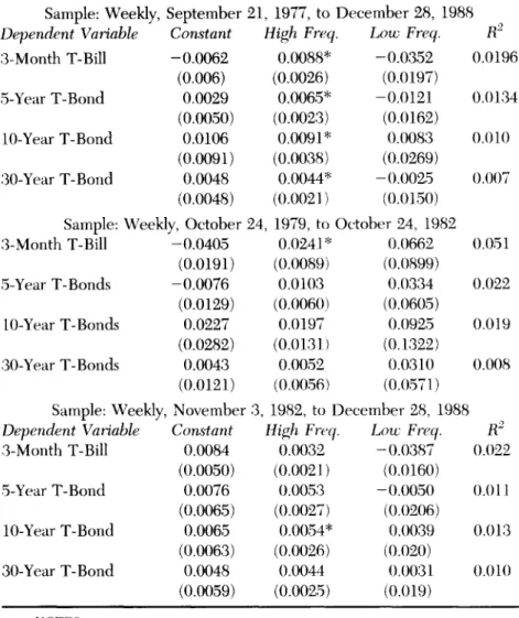
TABLE 4. Reaction of Nominal Yields to High vs. Low Frequency Components of Unanticipated Money

Sample: Weekly, September 21, 1977, to December 28, 1988

Dependent Variable Constant High Freq. Low Freq. R ~

3-Month T-Bill -0.0062 (0.OO6) 5-Year T - B o n d 0.0029 (0.0050) 10-Year T-Bond 0,0106 (0.0091) 30-Year T-Bond 0,0048 (0.0048) Sample: Weekly, October 24,

3-Month T-Bill -0.0405 (0.0191) 5-Year T-Bonds -0.0076 (0.0129) 10-Year T-Bonds 0.0227 (0.0282) 30-Year T-Bonds 0.0043 (0.0121) 0.0088* (0.0026) 0.0065* (0.0023) 0.0091" (0.0038) 0.0044* (0.0021) 1979, to 0.0241 * (0.0089) 0.0103 O.OO60) 0.0197 (0.0131) 0.0052 (0.0056) -0.0352 0.0196 (0.0197) -0.0121 0.0134 (0.0162) 0.0083 O.OLO (0.0269) -0.0025 0.007 (0.0150) October 24, 1982 0.0662 0.051 (0.0899) 0.0334 0.022 (0.0605) 0.0925 0.019 (0.1322) 0.0310 0.008 (0.057l) Sample: Weekly, November 3, 1982, to December 28, 1988

Dependent Variable Constant High Freq. Low Freq. R e

3-Month T-Bill 0.0084 0.0032 - 0.0387 0.022 (0.0050) (0.0021) (0.0160) 5-Year T - B o n d 0.0076 0.0053 -0.0050 0.011 (0.0065) (0.0027) (0.0206) 10-Year T-Bond 0.0065 0.0054* 0.0039 0.013 (0.0063) (0.0026) (0.020) 30-Year T-Bond 0.0048 0.0044 0.0031 0.010 (0.0059) (0.0025) (0.019) NOTES:

b) Asterisk denotes statistical significance at 95% level.

c) The coefficients report the reaction of noininal yields to high frequency and low frequency components of unanticipated money during diflbrent observation periods. The components are derived by decomposition in the frequency domain.

(12)

Umit Erol and Erol M. Balka~

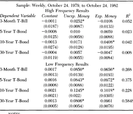
TABLE 5. Reaction of Nominal Yields' to Money Announcements-- Period of Targeting Non Borrowed Reserves

Sample: Weekly, October 24, 1979, to October 24, 1982 High Frequency Results

Dependent Variable Constant Unexp. Money Exp. Money R 2

3-Month T-Bill -0.0011 0.0252* -0.0108 0.052 (0.0187) (0.0087) (0.0133) 5-Year T-Bond -0.0008 0.010 0.0059 0.023 (0.0125) (0.0058) (0.0088) 10-Year T-Bond -0.0013 0.0171 0.0408* 0.042 (0.0274) (0.0128) (0.0195) 30-Year T-Bond -0.0004 0.0057 -0.0047 0.008 (0.0119) (0.0055) (0.0084)

Low Frequency Results

3-Month T-Bill 0.0017 0.0850* 0.0656* 0.268 (0.0013) (0.0139) (0.0193) 5-Year T-Bond 0.0016 0.0843* 0.0972* 0.375 (0.0008) (0.0088) (0.0122) 10-Year T-Bond 0.0021 0.1245" 0.1018" 0.228 (0.0021) (0.022) (0.030,5) 30-Year T-Bond 0.0013 0.0806* 0.0961 0.5848 (0.0005) (0.0054) (0.0076) NOTES:

b) Asterisk denotes statistical significance at the 95% level.

The high-frequency (short-run) results strongly contbrm to the predictions of the expected liquidity hypothesis. The innovations in the unexpected money supply explain only the post-announcement yield changes for the 3-month T-bills. The coefficient on the 3-month T-bill yields (0.025) is positive and appreciably higher than for any other period. A 1% increase in the unanticipated money supply raises the 3-month T-bill yields by 25 basis points in this specific period. None of the longer maturity yields displays significant responses to the unexpected money supply innovations. Further- more, the coefficients on long-term maturities (though insignificant) are characteristically lower than the coefficient on the 3-month T-bills. The expected money supply components are not significant.

This strong empirical support for the expected liquidity hypothesis observed in the high-frequency domain does not carry over to the low- frequency domain. The low-frequency results presented in Table 5 show

(13)

How Financial Markets Process Money lnfornuttion

significant and positive responses for all maturities to the unexpected money supply innovations. Short-term rates (T-bill yields) respond with a positive coefficient of 0.085. The 5-year, 10-year, and 30-year bond yields respond with positive coefficients of 0.084, 0.124, and 0.08, respectively. The coefficients on long-term maturities are as large as the coefficient on the short rate and considerably larger in one instance. Long-term bond yields increase in the same magnitude as the short rates in response to the announcement of an unanticipated surge in the money supply. The evidence in low-frequency domain is in strong conformity with the empirical predictions of the expected inflation hypothesis.

The results present a dilemma. The high-frequency results support the expected liquidity hypothesis while the low-frequency results support the expected inflation hypothesis. A meaningful synthesis of these conflicting results may be sought within the context of the combination hypothesis. It may be argued that both the expected liquidity and the expected inflation factors operated during this period. Financial markets assigned a larger weight to the expected liquidity factor in the short-run in light of the Fed's high credibility. Markets, however, also displayed a lack of confidence in the persistence of the policy of closely targeting non-borrowed reserves. These doubts, in fact, were fulfilled in 1982 when the Fed started to de-emphasize the monetary targets and abandoned the policy of targeting non-borrowed reserves. The reservations about the long-run credibility of the Fed (in terms of maintaining the monetary targets) led the market to adjust their expected long-run inflation rate. If this is so, we are faced with an asymmetrical picture. The market's short-run behavior is predominantly determined by expected liquidity factor, which explains the high-frequency evidence. However, the market's long-run reservations about the persistence of the Fed's policy kept long-run inflationary fears alive. So, the expected inflation factor still operated in the long-run. The innovations in long-run rates were essentially the result of this expected inflation factor, which is indicated by the strong, positive response of long-run rates in the low-frequency domain. It is noteworthy that this evidence is associated only with the low-frequency domain and only the low-frequency results display a picture in strong conformity with the expected inflation hypothesis. This is further evidence that the market was processing the information by different motives in the short versus the long run. 7 The

7This may shed some hght on the paradox mentioned in fi~otnote (6). The exchange rate movements are essential]y short-run in character and their behavior is more similar to the behavior of the short-nm interest rates rather than long-term rates. The empirical evidence in this paper seem to support the hypothesis that the exchange rates and short-term interest rates were predominantly driven by the expected liquidit T factor during the 1979-1982 period. The favorable evidence presented by Engel and Frenkel for the liquidity hypothesis was the result of this tact. Cornell's empirictd results (for similar periods) {;avoring the expected inflation

(14)

significant and positive coefficients on the expected m o n e y supply are puz- zling but may be explained by statistical reasons, s

I f the combination approach outlined above is correct, then it nmst be empirically s u p p o r t e d by the evidence from other periods. T h e F e d reverted to targeting b o r r o w e d reserves (instead o f n o n - b o r r o w e d reserves) with a closer eye on interest rate m o v e m e n t s in 1982. T h e period 1982-1988 is characterized by w e a k e r a d h e r e n c e to m o n e t a r y targets on the part of the Fed, which lowered the F e d ' s credibility in financial markets. As a result, we would normally expect the expected liquidity factor to be insignificant in this period. Empirical results (Table 6) confirm this. T h e coefficients on the u n e x p e c t e d m o n e y supply (including yield on 3 - m o n t h T-bills) are insignificant in the high-frequency regressions. T h e only exception is the significant and positive coefficient of the 10-year T - B o n d yields. T h o u g h the coefficient is small (0.005), it is still distinctly significant. T h e expected inflation factor replaces the expected liquidity factor in the short-run as well as the long-run. This factor, however, operates selectively and essentially centers on a 10-year horizon. T h o u g h this horizon is relatively long, this m a y p e r h a p s b e explained by the fact that the actual inflation rates were quite low in this period and there was not m u c h concern about n e a r - t e r m inflation. However, the observed deviations from m o n e t a r y targets and acceleration o f m o n e y growth rates still led the m a r k e t to assign a positive probability to possible inflationary surge in the long run and the expected inflation p r e m i u m s on 10-year T - b o n d yields w e r e adjusted u p w a r d as a result of this. '~

A puzzle is the significant but negative relation b e t w e e n the 3-Month T-bill yields and the u n e x p e c t e d m o n e y supply in low-frequency regressions.

hypothesis was demonstrating the pre-dominant role of the expected inflation factor in the long r u n .

SThe fact that the expected money supply is significant is not compatible with the efficiency of financial markets. We think that this is the result of high correlations between the announced money supply and the expected money supply series. The cross-correlations between these two series confirm this point. So the low-frequency results actually may reflect the effect of announced money rather than the expected money supply. The way that the series are constructed may lead to this result. The unanticipated money series are derived by subtracting the survey data (expected money) from tile announced money series and both series (expected and unexpected money) are the independent values of the regressions. This way of deri~dng the series (though conventional in announcement literature) does not permit a full orthogonalization of the variables. This especially plagues low-frequency estimates, which are obtained from a smaller sample (qnite a few periodogram ordinates). It may be interpreted as a cost we pay for the absence of very long series. The starting date of surveys (September 1977) nnfortunately limits the usable length of the series.

~Further evidence on this would be available if there were continuous series [br 5- or 10-year forward contracts. Unfortunately, such data are not available.

(15)

TABLE 6. Reaction of Nominal Yields to Money Ann~tncements Period of Targeting Borrowed Reserves'

Sample: Weekly, November 3, 1982, to December 28, 1988 High Frequency Results

Dependent Variable Constant Unexp. Money Exp. Money B z

3-Month T-Bill -0.0012 0.0024 0.0020 0.0083 (0.0049)

(0.002])

(0.0023) 5-Year T-Bond 0.00005 0.0052 -0.0001 0.011 (0.0064) (0.0027) (0.0030) 10-Year T-Bond -0.00004 0.0054* -0.0002 0.0133 (0.0062) (0.0027) (0.OO29) 30-Year T-Bond -0.00005 0.004 0.0016 0.011

(0.0058)

(0.OO25)

(0.0028) Low Frequency Results

3-Month T-Bill -0.00004 -0.0159" 0.0226* 0.3996 (0.0004)

(0.0013)

(0.0049) 5-Year T-Bond 0.000004 -0.0005 -0.0140" 0.014 (0.0005) (0.0017) (0.0064) 10-Year T-Bond 0.00007 0.0043* -0.0079 0.024 (0.0005) (0.0019) (0.0072) 30-Year T-Bond 0.00007 0.0040* 0.0005 0.012 (0.0006) (0.002) (0.0078) NOTES:

b) Asterisk denotes statistie~d significance at the 95% level.

This may have the following explanation. Short-term rates are driven by two components: inflationary expectations and expectations about the future course of real rates. These components have a strong tendency to offset each other. This negative correlation between the short-run forecasts of inflation and real interest rates has been demonstrated elsewhere (Campbell and Ammer 1993). Positive innovations of expected inflation tend to be associated with negative innovations in the real rates. If expectations about future inflation are relatively weak while the real rates are high (which was the case during most of the observation period), this may lead to the observed anom- aly. The fact that this is only observed in the low-frequency regressions may be related to the long-run characteristic of this event.

3. Conclusions

This paper introduces a novel technique to analyze announcement effects. Band spectrum regressions provide the opportunity, to test the effect

(16)

of money announcements in the short-run versus long-run. This property of band spectrum regressions is used to test the validity of the combination hypothesis. This hypothesis assumes that both the expected inflation factor and the expected liquidity factor may operate simultaneously in explaining the information processing behavior of financial markets. The relative weights of these factors depend on the perceived credibility of the Fed in adhering to monetary targets.

The empirical results support this view. The 1979-1982 period, which is characterized by a high degree of Fed credibility, presents a picture in which the effect of money announcements on yields is dichotomized. The expected liquidity factor determines the short-run expectations and behavior while the long-run expectations are shaped by the expected inflation factor. As the Fed reverses policy in later periods and allows larger deviations from targets, the expected liquidity factor which is strongly associated with the Fed's credibility disappears. In the absence of the expected liquidity factor, the expected inflation becomes the dominant concern in shaping both short- and long-run expectations. The long-run rather than the short-run inflationary expectations seem to be more important in the 1982-1988 period due to low inflation.

Received: October 1995 Final version: September 1996

References

Barro, Robert J. Macroeconomics. New York: John Wiley & Sons, Inc., 1984. Brunner, Karl, Alex Cukierman, and Allan Meltzer. "Stagflation, Persistent Unemployment and Performance of Economic Shocks." Journal of Mon- etary Economics 6 (1980): 467-92.

Campbell, John Y., and John Ammer. "What Moves the Stock and Bond Markets? A Variance Decomposition for Long Term Asset Returns.'" The Journal of Finance 48 (1993): 3-37.

Cornell, Bradford. "The Money Supply Announcement Puzzle: Review and Interpretation." American Economic Review 73 (1983): 644-67. Engel, Charles M., and Jeffrey A. Frankel. "Why Interest Rates React to

Money Announcements: An Explanation from the Foreign Exchange Rate Market." Journal of Monetary Economics 13 (1984): 31-39.

Engle, Robert. "Band Spectrum Regression." International Economic Re- view 15 (1974): 1-11.

Gilbert, Alton R. "Operating Procedures for Conducting Monetary Policy." Federal Reserve Bank of St. Louis Review (February 1985): 13-21.

(17)

Girton, Lance, and Dayle Natress. "Monetary Innovations and Interest Rates." Journal of Money, Credit and Banking 17 (1985): 289-97. Granger, Clive W., and Oskar Morgenstern. Predictability of Stock Market

Prices. Lexington, Mass.: Heath Lexington Books, 1970.

Hardouvelis, Gikas A. "Market Perceptions of Federal Reserve Policy and the Weekly Money Announcements." Journal of Monetary Economic.~ 14 (1984): 225-40.

McCallum, Bennett T. "On Low Frequency Estimates of Long Run Rela- tionships in Macroeconomics." Journal of Monetary Economics' 14 (1984): 3-14.

Nelson, Charles R., and Charles Plosser. "Trends and Random Walks in Macroeconomic Time Series: Some Evidence and Implications." Jonrnal of Monetary Economics 10 (1982): 139-62.

Sargent, Thomas J. Maeroeconomic Theory. New York: Academic Press, 1979.

Summers, Lawrence H. "Estimating the I_~ng Run Relationship Between Interest Rates and Inflation." Journal of Monetary Economics 18 (1986): 77-86.

Urich, Thomas, and Paul Wachtel. "The Effects of Inflation and Money Supply Announcements on Interest Rates." Journal of Finance 39 (1986): 1177-88.

Appendix

Let us assume that Yt and X t are covariance stationary processes. Also assume that the Yt and X t are related in time domain by the formula

Yt = ~ by X,_j + ~t = B(L) X t + ¢t, (1A) where E ¢t Xt-j = 0. Though Equation (1A) is the general specification, it is relatively easy to see that the standard regression format is a special case of the general specification with by = 0 for t = j and ~t satisfying E(et ¢tv/) = 0

and E(et "2) = o "z and E(et) = 0.

Let Cy{]) be defined as the autocovariance of process y in time domain according to

cy(]) = E(Y,L_;;. (2A)

If Cy{]) belongs to the space of square summable sequences L(o~, ~) then it can be shown that there exists a transformation (Fourier transform)

G,j(eh~) = ~ Crt(k) e i,,.k, (3A) which maps the space L ( - ~ , ~) one to one into the space L(-r~, 7z) defined on a unit circle and preserving the linear structure and the metric properties.

(18)

Applying similar translbrms to the inputs of" Equation (1A) leads to the frequency domain representation of Equation (1A) as

G!t(e-I,,-) = B(eh,,) B(e-l~,) Gx(e l,~.) + G~(e-t,~) , (4A) where Gy(e-Z'~), Gx(e h~,) and G,(e -h~) are Fourier translbrms applied to time domain series Yt, X~ and et respectively while B(e t'~) B(e -t'~,) is the Fourier transform applied to the lag operator. Alternatively, we can write (Sargent 1979)

Gy(e -l~) = [B(et'~)l e Gx(e -h~) + G,(e -h~) , (5A) using the symmetry properties of the spectrum and conjugate multiplication. The importance of Equation (5A) is in the fact that it shows how the spectrum of Y can be obtained from the spectrum of the input variable X by multiplying it with a non-negative real number IB(et'~)l z. One may replace the lag operator (which reduces to a trivial form in the case of ordinary regression) by an appropriate filter. In other words, the fact that IB(et":)l 2 is a non-negative real number operator allows us to define a filter B(e -h~) such that

B(e -m) = 1 for w ~ (a, b) and 0 otherwise ,

and use this filter in Equation (5A). Such a filter shuts off or masks all the spectral power for frequencies not in the region [a,b] and only letting the spectral power in the region [a,b] to pass through the filter.