Optimal filtering in fractional Fourier domains

OPTIMAL FILTERING IN FRACTIONAL FOURIER DOMAINS

M .

Alper Kutay, Haldun

M.

Ozaktas, Levent Onural, and Orhan Arzkan

Bilkent University, Department

of

Electrical Engineering

TR-06533 Bilkent, Ankara, Turkey

ABSTRACT

The ordinary Fourier transform is suited best for analysis and processing of time-invariant signals and systems. When

we are dealing with time-varying signals and systems, filter- ing in fractional Fourier domains might allow us t o estimate signals with smaller minimum-mean-square error (MSE). We derive the optimal fractional Fourier domain filter that minimizes the MSE for given non-stationary signal and noise statistics, and tiime-varying distortion kernel. We present an example for which the MSE is reduced by a factor of 50 as a result of filtering in the fractional Fourier domain, as compared t o jiltering in the conventional Fourier or time domains. We also discuss how the fractional Fourier trans- formation can be computed in O ( N log

N )

time, so that the improvement in performance is achieved with little or no increase in computational complexity.

1. INTRODUCTION

The fractional Fourier transform was defined mathemati- cally by Namias [2], and McBride and Kerr [3]. Its analog optical implementation was discussed in [4, 51 and recently a fast digital O ( N log

N )

time algorithm has also been de- veloped. (The outline of this algorithm will be given in the appendix.) Other work in this area includes [l] and [8] in which many properties are derived and applications are suggested.

SeveraJ applications of the fractional Fourier transform have been suggested or explored t o varying degrees. These include optical diffraction and beam propagation, optical signal processing, quantum optics, phase retrieval, signal detection, pattern recognition, noise representation, time- variant filtering and multiplexing, d a t a compression, study of space/time-frequency distributions [l, 2, 3, 4, 5, 7, 8, 91. The ai,h order fractional Fourier transform of a function, denoted by F ' " [ f ] ( z ) , is defined as [l, 31:

(FVI)

(z) =

Jp,

Ba(z, z')f(z') dz',

9 (1) t n ( x 2 c o t 4-211' csc ++3'2 c o t 4) Ba(z,z') = A4e

where A4 =

(I

sin

41)-"'

exp (i( rrS sin -

$))

,

and

4

a x / 2 . The kernel B a ( z , z ' ) approaches 6(z-z') or 6(z+z')

when a approaches 0 or f 2 , respectively. The definition is easily extended outside the interval [-2,2] since

F*

is the identity operation [ 3 ] .

Some essential properties of the fractional Fourier trans- form are: i) It is linear. ii) The first order transform ( a = 1)

corresponds t o the common Fourier transform.

iii)

It is ad- ditive in index,

3"'FU2

f = 3 a l t a 2 f .

An important property of the fractional Fourier trans- form is its relation t o the Wigner distribution. Let W ( z , U )

denote the Wigner distribution of the signal f . It is well known that the projection of W ( z , v ) onto the z axis gives the magnitude squared of the Gequency-domain represen- tation, and the projection onto the Y axis gives the magni- tude squared of the time-domain representation of the sig- nal. The property in question states that the projection onto an axis making angle

4

with the x-axis gives the mag- nitude squared of the a = $th order fractional Fourier transform of the function. This property can be formulated

as iv)

R+[W,(z,v)]

=

lFu[f]IZ,

where the operator 2 4 is the Radon transform evaluated at the angle

4.

Other prop- erties may be found in [l, 2 , 3, 4, 51.

The ordinary Fourier transform is suited best for anal- ysis and processing of time-invariant signals. When we are dealing with time-varying signals and systems, filtering in fractional Fourier domains might allow us to estimate sig- nals with smaller minimum-mean-square error. In a simi- lar spirit, multiplexing in fractional Fourier domains allows signals whose time-frequency distribution is irregular t o be packed more efficiently in a given channel [l]. In this work we concentrate on filtering in fractional domains.

A /xm

NOISE

X

SIGNAL

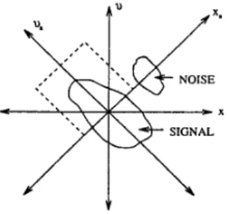
Figure 1: Noise separation in a=0.5th domain There are a variety of time-varying digital signal pro- cessing algorithms based on mixed time-frequency signal representations. (see for example [IO] and the references given there.) Many signal processing operations have been implemented by modifying these representations in some time-varying manner. However the majority of these suffer from especially two problems: i.) Most of the representa- tions, such as the Wigner distribution, are not linear so that there exists interference terms for multicomponent signals ii.) T h e modified time-frequency representation may not be

0-7803-2431

6/95

$4.00

0 1995

IEEE

the time-frequency representation of any signal, so that ad hoc approximations must be introduced.

Recently we have discussed how various space-variant operations can be performed by multiplying with a filter function in a fractional Fourier domain [I]. Signals with significant overlap in both the time and frequency domains may have little or no overlap in a fractional Fourier do- main. To understand the basic idea in the simplest possible terms, consider the simple example shown in figure 1, where the Wigner distributions of a desired signal and undesired distorcion term are shown. By virtue of property iv), we observe that they overlap in both the a=Oth and a=lst do- mains (consider the projections on the z and I/ axes), but

they do not overlap in the a = 0.5th domain. Thus we can eliminate undesired signal components by using a simple unit amplitude mask in the a = 0.5th domain.

2.

PROBLEM STATEMENT AND SOLUTION

We consider a commonly used signal observation model,

y = H ( z ) + n, (2)

where

X(.)

is a linear system that degrades the input (de- sired) signal x, and n is an additive noise term. Our aim is t o filter the observed signal y to minimize the effects of degradation and noise. Our criteria for judging the effec- tiveness of the restoration is t h e mean square error (MSE). We will assume t h a t as a prior knowledge we know the cor- relation functions

R,,(t,

t‘)

=

E [ z ( t )

~ ( t ’ ) ] ,

R,,,(t,t’) =

E [ n ( t ) n(t’)] of the input process and noise. We will fur- ther assume that the noise is independent of the input and it is zero mean for all time, i.e. E [ n ( t ) ] = 0 V t . Under these assumptions we can also compute the cross correla- tion function R,,(t, t’) = E [ z ( t ) y(t’)] of the input process

z and the output process y, and the correlation function R,,(t, t’) = E [ y ( t ) y ( t ’ ) ] of the output process by virtue

of equation 2. Now, consider a linear estimate of the form 5 =

G

(y). T h e corresponding MSE is

where

11. I l2

denotes the L2 norm of the signal. For the above definition of the MSE to be meaningful, we require the input processes and noise t o be square-integrable. This in turn ne- cessitates the input processes and noise t o be non-stationary. For stationary processes the MSE is simply defined as the expected value of the absolute value of the difference term. For the time-invariant degradation model 31 with sta- tionary processes x and n , the linear operator P,t that minimizes the MSE corresponds t o the optimal Wiener fil- ter. In this case, the required operation turns out to be of the convolution type, so that one can effectively imple- ment it with a filter in the conventional Fourier domain. For an arbitrary degradation model or for non-stationary pro- cesses, finding the general linear filter that minimizes the

MSE is difficult. More importantly, in general the resulting linear filter will be time-variant (not expressible as a convo- lution), so that it cannot be implemented in Nlog N time using FFT based techniques.

We consider filters in the fractional Fourier domain, that is, the estimated signal is related t o the observation as,

03

=

J_,

B-,(t, t’) g ( t ’ )

Jp,

B,(t’, t ” ) y ( t ’ ’ ) dt” dt’

This filter corresponds t o multiplication with a function g ( . )

in the a t h domain. If a = 1, this corresponds t o Fourier do- main filtering as in the case of Wiener filtering. With this form of estimation filter, the minimization problem consid- ered in this paper can be formally written as:

gopt ( t ) = a r g min a: (3)

9

The class of fractional Fourier domain filters is still a subclass of the class of

all

linear filters, so the linear filter we find will not be optimal among all linear filters. How- ever, it is a much broader class than time-invariant Fourier domain filters, and in some cases it is possible t o reduce the MSE for time-varying degradation models or non station- ary processes, as compared t o filtering in the conventional Fourier domain. T h e resulting filter can be implemented ef- ficiently since efficient optical and digital implementations of the fractional Fourier transform are known.

We will attempt t o solve the minimization problem de- fined by equation (3) using calculus of variations method. We define the cost function J = a:. J varies with the choice of g(.) since 2 ( t ) varies. This functional J is t o be minimized with respect to g ( . ) . We substitute g ( . ) = go(.)

+

a s g o ( . ) where a = are

+

4 ( Y ; ~ is a complex scalar parameter, go(.) is the optimum filter and 6go(.) is an arbitrary perturbation term and we fix go(-) and 6 g o ( . ) . With this substitution

2 ( t ) and also J vary with a for each fixed tigo(.),

00 2

( t ,

a) =

J_,

B-a(t, t’) ( g o ( t ‘ >

+

( a r e

+

i a t m ) sgo(t’)) rcw x

/

Ba(t’, t”)y(t”) dt” dt‘ J - C O

I

( ~ ( t ) - ? ( t , a)) ( z ( t ) - 5 ( t , CY))* d t

T h e necessary conditions for the optimum value of J are

[Ill:

(4) It can be shown that after some algebraic manipulations, the necessary conditions for optimality of J imply,

E

[Ll

6 g d t ’ )

(11

( 4 t ) - ? ( t , O ) ) *

B-,(t, t ’ )

1;

B,(t’, t ” ) y ( t ” ) dt” at

)

dt‘] = 0

(5) Since 6 g 0 ( t ’ ) is an arbitrary term and equation (5) is true for

all 6 g o ( t ’ ) , the inner integral should be equal to zero. Using this condition one can find the optimal filter function:

( 6 ) where the correlation functions are defined as R,, ( t , t ” ) = E [ z ( t ) y * ( t ” ) ] and R,,(t, t ” ) = E [y(t)y*(t”)].

P

( i ] = F - a ( g . P ( y ) ) ( t )

In the above formulation, it was assumed that the value of a is given. To find the optimal choice of a, we can substi- tute the olptimuni filter function (cf. ( 6 ) ) into the definition of MSE and apply a minimization algorithm with respect t o

a. In practice, it might be easier to find the optimum value

of a by computing the MSE as a function of a , and choosing that value of a which results in the smallest MSE.

D i s c r e t e t i m e f o r m u l a t i o n . We now present the dis- crete time formullation, beginning directly from the discrete version of Eq. 2 . In this case

H

is a matrix and 2 , n, and

y are vectors. They will be denoted by underlined bold- face letters from now on. The discrete fractional Fourier transform takes on the form of a matrix multiplication (see appendix), just 21s the ordinary discrete Fourier transform.

The error for the discrete case is given by:

where N is the size of the input vector

x

and

4

=

z-"&ga

E.

Here A is a diagonal matrix whose diagonal consists of el- ements of the vector g

,

and

Ea

is the fractional Fourier transformation matrix- The inverse transformation matrix is - =

(Ea)",

since the fractional Fourier transforma- tion is unitary. Here

(.)*

denotes conjugate transpose.

This estimate corresponds t o a multiplicative filter in the a t h fractional Fourier domain. As in the continuous time case, if a = 1,

Fa

is simply the D F T matrix and we obtain the common E u r i e r domain filter.

In order t o find the optimal filter that minimizes the MSE, we define the cost function J d = U: and note that

it varies with the choice of the vector g = [gi gz

...

g ~ ] . Since in general the filter vector - g can Fe complex, we can write its components as g, =

+

i

gi,im. T h e optimum value of the cost function J d is obtained from the conditions,

=g

It can be shown that the elements of the optimum filter function are given by,

where l&,=

E: [xu"]

,

gYy

=

E

[zzH]

are the corre- lation mat.rices and f a H is the j t h row of the matrix

Fa.

-

This last equation provides the solution of our minimiza- tion problem in the discrete time setting. We note that this result is fully analogous t o the solution obtained in equation (6) for the continuous time case.

-J

3. EXAMPLE

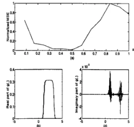
In this section, computer simulations that illustrate the ap- plications and performance of our filtering scheme will be given. We consider a degradation model that corresponds to a time-varying, low-pass filter whose bandwidth increases linearly in time. The input process is a Gaussian function which deterministic except for a random amplitude. The

noise process is finite duration bandpass noise which is mod- ulated with an exponential quadratic chirp function ( e - 1 p t z ) so that its center frequency increases linearly with time. In Fig. 2 (a), we have shown the normalized MSE plot for dif- ferent values of a. From the plot we find that the minimum

MSE

is achieved for a = 0.5. We have plotted the real part of the optimum filter function for a = 0.5 in Fig. 2 (b) and the imaginary part in (c). We note that the imaginary part can be set t o zero without effecting the final results. Fig.

3 (a) and (b) shows realizations of the input and output processes (only real part is plotted) respectively. Resulting estimates for these realizations are plotted in Fig. 3 (c). The

MSE is 0.001 for a = 0.5 while it is 0.063 for a = 1.

= 02

0.1 0.2 oa 0.4 os 0.6 0.1 0.8 o o 1 a (4

I

Figure 2: (a) MSE vs a, (b) Real part of optimal filter in a=0.5th domain (c) Imaginary part

0.5

ll

/ / I

. .

.

.

. .

Figure 3: (a) Realization of input process I , (b) Realization of process y (c) Comparison of the estimate 2 in the 0.5th domain (dashed), the estimate 3 in the 1st domain (dotted) and the I (solid)

4. CONCLUSION

Filtering in fractional Fourier domains may enable signif- icant reduction of the MSE compared t o ordinary Fourier domain filtering. This reduction comes at essentially no ad- ditional cost, since the fractional Fourier transform has an

O ( N log N ) algorithm. We have presented a mathematical formulation and solution of this problem analogous to the formulation and solution of the the optimal Wiener filtering problem.

Filtering in fractional domains will work better for cer- tain kinds of distortions and signal and noise statistics in comparison to others. The presence of time-varying distor- tion and non-stationary statistics suggest that the fractional transform may be of use, but do not guarantee significant improvements in every case.

The method can be greatly improved by filtering in not one, but several consecutive fractional Fourier domains. This not only allows one to handle a much wider variety of signals, but may also create the potential to approximate the most general optimal linear filter

5 .

APPENDIX

In this appendix, we present a fast algorithm for the im-

plementation of the fractional Fourier transformation. The definition of the fractional Fourier transformation can be cast in the form,

00

e -127rpzz' [ e i m a z " f ( z ' ) ] dz', (10)

L

r F " [ f ] ) (x) = A.+erTUzz

where a = cot and /3 = cscd. The last term inside the integral corresponds to a chirp modulation of the signal

f(.).

This modulation results in a vertical shear in the Wigner domain since the Wigner distribution of a chirp signal is a

line delta [SI.

It will be assumed that the Wigner distribution o f f ( - ) is negligibly small outside a circle of diameter A z centered around the origin. (Az must be chosen large enough to satisfy this assumption. Normalizing the axes so that the spread of the Wigner distribution is approldmately identi- cal along both axes wiU allow smaller choices of Az, which wiU reduce computational complexity. These are essentially the same considerations that go onto approximating a con- tinuous Fourier transform with the

DFT.)

Under this as- sumption, and by limiting

6

to the interval

f

<

4

<

p,

the amount of vertical shear in the Wigner domain result- ing from chirp modulation is bounded by

+.

This ensures that the modulated function f ( x ' ) is bandlimited t o A x in the frequency domain. This allows f(.) to be repre- sented by Shannon's interpolation formula as follows:

N

n = - N

(11) where N is the largest integer smaller than (Ax)'. The summation ranges from - N to N since f(z') is assumed

t o be negligible outside that interval. By using Eq. 11 and

r q . 10 and changing the order of integration and summation

we obtain:

where we made use of

s_",

e-i2aPzz' sinc ( 2Ax ( z

'

-

&>>

d x

'

= formed function are obtained by:

e - I 2 nj3-7

-

&rect(&) ; Then the samples of the trans-

*=-N

Direct computation of the above matrix-vector product would require O ( N 2 ) multiplications. An

O(N

log N ) algorithm for the computation of this form can be readily obtained. For this purpose, we put Eq. 13 into the following form after some algebraic manipulations:

N

n = - N

It can be recognized that the summation corresponds to a convolution of etrP( with the chirp modulated function

f(.). The standard FFT can be used to compute this con-

volution in O(N1og

N)

time. The output samples are then obtained by another chirp modulation. Hence the overall time complexity is O ( N 1 o g N ) . The factor r e c t ( 2 ) only limits the length of the output signal.

5

(b

5

5

and

--;

5

4

5

-9

(0.5

5

a

5

1 and -1

5

a

5

-0.5). However

using a basic property of the fractional Fourier transform we can extend this range to all values of a. For example:

F a

=

The above presented method is not the only one which results in O(N1og N ) computation. However, it has many desirable features compared to other methods of decompos- ing the chirp integral and leads to good numerical behavior.

This algorithm is valid only for

= ga-'T1

,

0

5

a

5

0.5 etc.

6.

REFERENCES

[l]

H. M.

Ozaktas, B. Barshan,

D.

Mendlovic, and

L.

Onu-

[2] V. Namias. J. Inst. Maths Applics.,25:241-245,1980. [3]

A.

C.

McBride and

F.

H. Kerr. I M A J . Appl. Math., [4] H. M. Ozaktas and D. Mendlovic. Opt. Commun.,

[5]

A.

W. Lohmann. J. Opt. Soc. Am. A , 10:2181-2186, [6] T.

A.

C.

M.

Claasen and W. F. G. Mecklenbraucker.

[7]

H. M.

Ozaktas,

D.

Mendlovic," Fractional Fourier Op-

183 L.

M.

Almeida. Proceedings of ICASSP 1993, 111-257. [9]

J.

R.

Fonollosa and C. L. Nikias.Proceedings of ICASSP

[IO] B.

E .

A. Saleh and N. S. Subotic. IEEE Trans. ASSP.,

[ll] G.M. Ewing, Calculus of Variations with Applications.

ral. J. Opt. Soc. A m . A , 11:547-559, 1994.

39:159-175, 1987. 101:163-169, 1993. 1993.

Philips Journal of Research, 35:217-250,1980.

tics," to appear in JOSA A .

1994, IV-301-IV-304.

~01.33, no.6, pp.1479-1485,Dec. 1985.

Dover publications, 1985.