Indoor multi-person tracking via ultra-wideband radars

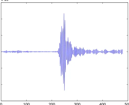
The designed antenna is used to transmit a second derivative Gaussian pulse and the received third order Gaussian like signal is as shown in Figure

Kıym etli üstat doktor general Besim Ömer

Yavaş piroliz ile daha çok katı ürün elde edilirken, alternatif sıvı yakıtlara duyulan ihtiyacın artmasıyla birlikte, yüksek ısıtma hızlarıyla sıvı

The parameters required for the lumped equivalent circuit of Mason are shunt input capacitance, turns ratio and the mechanical impedance of the membrane. Of course the collapse

We also wish to make a clear distinction between the collective modes generated by the single-particle excitations between dierent Landau levels, also known as

We demonstrate red-shifting absorption edge, due to quantum confined Stark effect, in nonpolar InGaN/GaN quantum structures in response to increased electric field, while we show

Tamiolaki (eds.), Thucydides between History and Literature (Berlin 2013) 73–87, at 80–81, also notes the traditional joining of limos and loimos and suggests that Thucydides

To determine the impact of news shocks on inbound tourism demand to Turkey, this study investigated the tourist arrival rates (the growth rate of arrivals or, in other words,

Bibliography

[1] Z. Sahinoglu, S. Gezici, and I. Guvenc, Ultra-Wideband Positioning Systems: Theoretical Limits, Ranging Algorithms, and Protocols. Cambridge, U. K, 2008.
[2] http://www.timedomain.com/
[3] W. Dargie and C. Poellabauer, Fundamentals of Wireless Sensor Networks: Theory and Practice. John Wiley and Sons, 2010.
[4] K. Sohraby, D. Minoli, and T. Znati, Wireless Sensor Networks: Technology, Protocols, and Applications. John Wiley and Sons, 2007.
[5] J.-Y. Lee and R. Scholtz, “Ranging in a dense multipath environment using an UWB radio link,” IEEE J. Sel. Areas Commun., vol. 20, pp. 1677–1683, Dec 2002.
[6] M. Chiani and A. Giorgetti, “Coexistence between UWB and narrow-band wireless communication systems,” Proceedings of the IEEE, vol. 97, pp. 231– 254, Feb 2009.
[7] R. Zekevat and R. Buehrur, Wireless Localization Using Ultra-Wideband Signals, 1st ed. New York, NY, USA. Wiley-IEEE Press, 2012.
[8] D. Dardari, A. Conti, U. Ferner, A. Giorgetti, and M. Win, “Ranging with ultrawide bandwidth signals in multipath environments,” Proceedings of the IEEE, vol. 97, pp. 404–426, Feb 2009.
(48)
[9] S. Gezici, Z. Tian, G. Giannakis, H. Kobayashi, A. Molisch, H. Poor, and Z. Sahinoglu, “Localization via ultra-wideband radios: a look at position-ing aspects for future sensor networks,” IEEE Signal Processposition-ing Magazine, vol. 22, pp. 70–84, July 2005.
[10] B. Sobhani, M. Mazzotti, E. Paolini, A. Giorgetti, and M. Chiani, “Effect of state space partitioning on bayesian tracking for UWB radar sensor net-works,” in IEEE International Conference on Ultra-Wideband (ICUWB), pp. 120–125, Sep. 2013.
[11] B. Sobhani, E. Paolini, A. Giorgetti, M. Mazzotti, and M. Chiani, “Bayesian tracking in UWB radar sensor networks,” in IEEE International Conference on Communications Workshops (ICC), pp. 47–51, June 2013.
[12] S. Bartoletti, A. Conti, and A. Giorgetti, “Analysis of UWB radar sensor networks,” in IEEE International Conference on Communications (ICC), pp. 1–6, May 2010.
[13] M. Svecova, D. Kocur, R. Zetik, and J. Rovnakova, “Target localization by a multistatic UWB radar,” in 20th International Conference on Radioelek-tronika (RADIOELEKTRONIKA), pp. 1–4, April 2010.
[14] X. wei Zhao, A. Gaugue, C. Liebe, J. Khamlichi, and M. Menard, “Through the wall detection and localization of a moving target with a bistatic UWB radar system,” in European Radar Conference (EuRAD), pp. 204–207, Sept 2010.
[15] G. Wei, Y. Zhou, and S. Wu, “Detection and localization of high speed moving targets using a short-range UWB impulse radar,” in IEEE Radar Conference (RADAR 2008), pp. 1–4, May 2008.
[16] D.-H. Kim, D.-W. Lim, L. Shen, H.-M. Kim, S.-C. Woo, and H. K. Yu, “Localization methods of multi-targets for UWB radar sensor networks,” in 3rd International Asia-Pacific Conference on Synthetic Aperture Radar (APSAR), pp. 1–4, Sept 2011.
(49)
[17] H. Ding, C. Chen, S. Peng, X. Li, and L. Zheng, “Multistatic ultra-wideband localization for NLOS environments,” in Second International Conference on Intelligent System Design and Engineering Application (ISDEA), pp. 380– 384, Jan 2012.
[18] S. Balckman and R. Popoli, Design and Analysis of Modern Tracking Sys-tems. Norwood, MA, USA: Artech House, 2010.
[19] R. Mahler, Statistical Multisource-Multitarget Information Fusion. Artech House, 2007.
[20] R. Mahler, “Multitarget Bayes filtering via first-order multitarget moments,” IEEE Trans. Aerosp. Electron. Syst., vol. 39, no, vol. 39, p. 11521178, Oct. 2003.
[21] M. S. Arulampalam, S. Maskell, N. Gordon, and T. Clapp, “A tutorial on particle filters for on-line nonlinear/non-Gaussian Bayesian tracking,” in IEEE Trans. Signal Process, vol. 50, 2002.
[22] B. Ristic, S. Arulampalam, and N. Gordon, Beyond the Kalman filter: Par-ticle filters for tracking applications. Artech House, 2007.
[23] F. Gustafsson, “Particle filter theory and practice with positioning applica-tions,” in IEEE Aerosp. Electron. Syst. Mag., vol. 25, 2010.
[24] S. Jovanoska and R. Thoma, “Multiple target tracking by a distributed UWB sensor network based on the PHD filter,” in 15th International Conference on Information Fusion (FUSION), pp. 1095–1102, July 2012.
[25] B. Sobhani, E. Paolini, A. Giorgetti, M. Mazzotti, and M. Chiani, “Tar-get tracking for UWB multistatic radar sensor networks,” IEEE Journal of Selected Topics in Signal Processing, vol. 8, pp. 125–136, Feb 2014.
[26] S. Jovanoska, R. Zetik, R. Thoma, F. Govaers, K. Wilds, and W. Koch, “Device-free indoor localization using a distributed network of autonomous UWB sensor nodes,” in Workshop on Sensor Data Fusion: Trends, Solutions, Applications (SDF), 2013, pp. 1–6, Oct 2013.
(50)
[27] Y. Kilic, H. Wymeersch, A. Meijerink, M. Bentum, and W. Scanlon, “Device-free person detection and ranging in UWB networks,” IEEE Journal of Se-lected Topics in Signal Processing, vol. 8, pp. 43–54, Feb 2014.
[28] Y. Zhou, C. L. Law, Y. L. Guan, and F. Chin, “Localization of passive target based on UWB backscattering range measurement,” in IEEE Int. Conf. on Ultra-Wideband (ICUWB), pp. 145–149, Sep. 2009.
[29] W.-K. Ma, B.-N. Vo, S. Singh, and A. Baddeley, “Tracking an unknown time-varying number of speakers using TDOA measurements: a random finite set approach,” IEEE Transactions on Signal Processing,, vol. 54, pp. 3291–3304, Sept 2006.
[30] B.-N. Vo, S. Singh, and W.-K. Ma, “Tracking multiple speakers using random sets,” in IEEE International Conference on Acoustics, Speech, and Signal Processing (ICASSP), vol. 2, pp. ii–357–360, May 2004.
[31] J.-M. Valin, F. Michaud, and J. Rouat, “Robust 3D localization and tracking of sound sources using beamforming and particle filtering,” in IEEE Inter-national Conference on Acoustics, Speech and Signal Processing (ICASSP), vol. 4, pp. IV–IV, May 2006.
[32] First Report and Order 02-48, “Federal Communications Commissions,” Feb. 2002.
[33] Y. Bar-Shalom, X. R. Li, and T. Kirubarajan, Estimation with Applications to Tracking and Navigation. John Wiley, 2001.
[34] B.-N. Vo and W.-K. Ma, “The Gaussian mixture probability hypothesis den-sity filter,” IEEE Transactions on Signal Processing,, vol. 54, pp. 4091–4104, Nov 2006.
[35] B. N. Vo, S. Singh, and A. Doucet, “Sequential Monte Carlo implementation of the PHD filter for multi-target tracking,” IEEE Trans. Aerosp. Electron. Syst., vol. 41, no, vol. 41, no. 4, p. 12241245, 2005.
[36] B. Ristic, D. Clark, and B. Vo, “Improved SMC implementation of the PHD filter,” 2010.
(51)
[37] E. Ozkan, M. B. Guldogan, U. Orguner, and F. Gustafsson, “Ground multi-ple target tracking with a network of acoustic sensor arrays using PHD and CPHD filters,” IEEE Int. Conf. Information Fusion (FUSION), 2011.
[38] M. B. Guldogan, U. Orguner, and F. Gustafsson, “Gaussian mixture PHD filter for multi-target tracking using passive Doppler-only measurements,” in 9th IET Data Fusion Target Tracking Conference (DF TT 2012): Algorithms Applications, pp. 1–6, May 2012.
[39] M. B. Guldogan, D. Lindgren, F. Gustafsson, H. Habberstad, and U. Orguner, “Multi-target tracking with PHD filter using Doppler-only mea-surements,” Digital Signal Process., vol. 27, pp. 1–11, April 2014.
[40] D. Clark, B. N. Vo, and J. Bell, “GM-PHD filter multitarget tracking in sonar images,” in SPIE Proc. SPIE Defense and Security Symposium, 2006.
[41] M. Ulmke, O. Erdinc, and P. Willett, “GMTI tracking via Gaussian mix-ture cardinalized probability hypothesis density filter,” IEEE Trans. Aerosp. Electron. Syst., vol. 46, pp. 1821–1833, Oct. 2010.
[42] D. Laneuville and J. Houssineau, “Passive multi target tracking with GM-PHD filter,” in IEEE Int. Conf. Information Fusion (FUSION), 2010. [43] R. Georgescu and P. Willett, “The GM-CPHD tracker applied to real and
realistic multistatic sonar data sets,” IEEE Journal of Oceanic Engineering, vol. 37, pp. 220–235, Apr. 2012.
[44] M. Pace, “Comparison of PHD based filters for the tracking of 3D aerial and naval scenarios,” in IEEE Radar Conference, pp. 479–484, 2010.
Şekil
Figure 2.1: Applications and business opportunities for low rate UWB systems [1].
Figure 2.3: Indoor environment with four radar sensors. Blue signals and red signals represent transmitted and received signals, respectively.
Figure 2.4: Illustration of the interface to a P410 MRM [2].
Figure 2.6: Configuration window [2].
+7
Referanslar
Benzer Belgeler