Cell-graph mining for breast tissue modeling and classification

Cell-Graph Mining for Breast Tissue Modeling and Classification

Cagatay Bilgin

, Cigdem Demir

,Chandandeep Nagi

, Bulent Yener

.

a

_{Department of Computer Science, Rensselaer Polytechnic Institute, Troy, NY 12180, USA.}

_{Department of Computer Engineering, Bilkent University, Ankara, Turkey.}

c

_{Mount Sinai Medical Center, NY 10029, USA.}

Abstract— We consider the problem of automated cancer

diagnosis in the context of breast tissues. We present graph theoretical techniques that identify and compute quantitative metrics for tissue characterization and classification. We seg-ment digital images of histopatological tissue samples using k-means algorithm. For each segmented image we generate different cell-graphs using positional coordinates of cells and surrounding matrix components. These cell-graphs have 500-2000 cells(nodes) with 1000-10000 links depending on the tissue and the type of cell-graph being used. We calculate a set of global metrics from cell-graphs and use them as the feature set for learning. We compare our technique, hierarchical cell graphs, with other techniques based on intensity values of images, Delaunay triangulation of the cells, the previous technique we proposed for brain tissue images and with the hybrid approach that we introduce in this paper. Among the compared techniques, hierarchical-graph approach gives 81.8% accuracy whereas we obtain 61.0%, 54.1% and 75.9% accuracy with intensity-based features, Delaunay triangulation and our previous technique, respectively.

I. INTRODUCTION

Breast cancer is the most common cancer and the second leading cause of cancer death among American females. The current incident rates predict that 1 in 8 women in the United States will develop breast cancer in their lifetime. Currently, long-term survival is approximately 70%. The diagnosis and staging for prognosis is based on histopathological examination and grading of surgically removed breast tissue and axillary lymph nodes which depends on established clinical, and laboratory parameters such as histopatological grading and hormonal receptor status of individual tumor tissues. Unfortunately, these parameters are only accurate in approximately 75-80% of the cases, particularly in Stage I tumors. In this group of patients, despite being node negative i.e. tumor confined to the breast with no spread to lymph nodes, 20-30% will recur. Thus, it is important to be able to predict which group of these patients will need chemotherapy to prevent tumor recurrence.

Current techniques for diagnosing and predicting the bi-ological behavior of cancer in individual patients are based predominantly on pathological parameters. New molecular techniques are currently being utilized to identify higher risk for specific subgroups of cancer and are in great demand. Unfortunately, reliable prognostic information is still not available in a significant percentage of individuals with common types of cancer, such as breast cancer.

A large set of automated cancer diagnosis tools exists in literature which are based on learning some feature sets.

Morphological features such as area, perimeter, and round-ness of a nucleus are used in [7], [3], [9] for this purpose. Textural features such as the angular second moment, inverse difference moment, dissimilarity, and entropy derived from the co-occurrence matrix are used for diagnosis in [3], [4]. To distinguish the healthy and cancerous tissues these systems are trained by using artificial neural networks [4], the k-nearest neighborhood algorithm, [7], support vector machines [3], linear programming, logistic regression, fuzzy, and genetic algorithms. Complimentary to the morphological and textural features, a few of these studies use colorimetric features such as the intensity, saturation, RGB components of pixels [7] and densitometric features such as the number of low optical density pixels in an image [4]. Another subset of these studies uses fractals that describe the similarity levels of different structures found in a tissue image over a range of scales [2]. Gabor filters that respond to contrast edges and line-like features of a specific orientation is presented in [1]. There are also techniques that rely on gene expression [6] and mass spectroscopy [12] to detect a cancer tumor. However, these tools require high technological hard-wired such as micro-arrays or mass spectrometers [6], [10].

There are also other approaches that construct a graph of cells from a tissue image and compute graph theoretical features to quantify how the cells are distributed over the tissue [5], [11], [14]. In these approaches, a graph of a tissue is defined by representing nuclei as vertices and defining edges to capture relationships between nuclei and graph metrics computed which are fed to the learning algorithms.

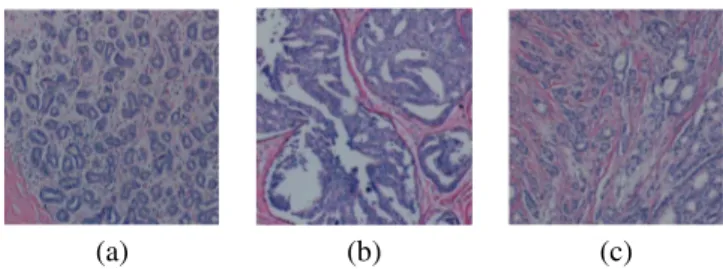
(a) (b) (c)

Fig. 1. Microscopic images of tissue samples surgically removed from human breast tissues: (a) a benign tissue example, (b) an in-situ tissue example, (c) an invasive tissue example.

II. METHODOLOGY

Our technique consists of segmenting the image to extract the cells, modelling the tissue by graphs according to the location of the cells and then learning these graphs using machine learning techniques. Each step is further discussed in the following sections.

Proceedings of the 29th Annual International Conference of the IEEE EMBS

Cité Internationale, Lyon, France August 23-26, 2007.

SaC06.5

A. Image Segmentation

1) Segmentation: In order to form graphs on top of the cells, first we need to segment the cells in tissue images. However, image segmentation is still an open question and there are several segmentation techniques that are proposed for different types of images. K-means algorithm, which clusters the pixels of images according to their RGB values into clustering vectors, gave satisfactory results for breast tissue images. This step is depicted as the transition from figure 2a to 2b. 2) Node Identification: We placed a grid on the resulting images of segmentation to identify the cells. For each grid entry we calculated the probability of being a cell as the ratio of cell pixels to the total number of pixels in the grid. Then we applied thresholding to decide whether this grid entry is a cell or not. The threshold value should be optimized to both identify the cells and eliminate the noise in the image. The result of node identification is given in figure 2d.

B. Cell-Graph Generation

After the image segmentation, we have the locations of the cells which are the centers of the grid entries. We build our graphs on top of these grid entries. After image segmentation step we have the vertex set of the graphs and in cell-graph generation we form the edges of the graphs. We constructed three different kinds of cell-graphs capturing the pairwise distance relationship between the nodes. These three different kinds of cell-graphs are explained in the following sections. 1) Simple Cell-Graphs: In simple cell-graphs we set a link between two nodes if the euclidean distance is less than a threshold. That is simple cell-graphs form a relation between nodes if they are close to each other.

2) Probabilistic Cell-Graphs: Probabilistic model is a more general version of simple cell-graphs. In this model we build a link between two nodes with a decaying probability as a function of euclidean distance between the nodes. These graphs do not necessarily form links between two nodes even if the distance between the nodes is small. Yet, it is more likely for the nodes that are close to each other will be linked while the nodes that are farther away will not be linked.

3) Hierarchical Cell-Graphs: The previous two forms of graphs capture the global distribution of the cells and were particularly useful for brain tissue images. However, there is an underlying architectural difference between the brain and breast tissues. Breast tissues have lobular archi-tecture whereas brain tissues do not have such higher level structures. For breast tissues, the pairwise relationship of cells within the same gland as well as different glands are therefore important. To capture the lobular architecture of the breast tissues we need an hierarchical representation of the tissues. We formed our hierarchical graphs similar to the way we formed our cell-graphs. After the node identification step we had our nodes (cells) of the graphs. In order to find the clusters (lobes) of the tissues, a grid is placed on top of these cells. Diving the number of cells in a grid by the grid size, we calculated the probability of being a cluster for each

grid entry. Then we set a threshold value and considered the grid entries having a probability greater than this threshold as a cluster. We then formed our graphs on these clusters. This step is depicted in figure 2e.

C. Cell-Graph Mining

In order to learn the differences between the graphs we need to find a way to extract the properties (metrics) of these graphs. The metrics that are computed for each graph are explained in section III. After calculating our metrics prior to learning, the metrics are scaled since some metrics are too large and some of them are too small therefore effecting the learning significantly. We scaled each metric to the range [−1, 1] for a better comparasion. We have used support vector machines (SVM) as our main classifier with a radial basis kernel. In order to find out the best parameters for the SVM we applied grid search on the training data.

III. METRICS

In order to have a quantitative representation of the graphs, we extracted some metrics from the graphs. The simplest metrics are the number of nodes in the graph and average

degree of a node. clustering coefficient of a node Ci is

defined as Ci= (2Ei)/(k(k + 1)), where k is the number of

neighbors of the node i and Eiis the number of existing links

between its neighbors. This metric quantifies the connectivity information in the neighborhood of a node. The path length between two nodes is defined as their shortest path length in the graph, taking the weight of each link as a unit length. Given shortest path lengths between a node i and all of the reachable nodes around it, the eccentricity and the closeness of the node i are defined as the maximum and the average of these shortest path lengths respectively. The maximum value of the eccentricity, the diameter of a graph, is another metric for the classifier. Central points of the graph is defined as the points having an eccentricity equal to the radius. This set of metrics reflects the centrality of the node.

For hop h, the hop plot value is defined as the number of node pairs such that the path length between these node pairs is less than or equal to h hops. Using the hop plot value distributions we compute effective diameter and hop-plot

exponent, which is the slope of the hop plot values as a

function of h in log-log scale. Giant connected component

ratio, percentages of isolated and end nodes are the last

set of metrics. A node of a graph is called isolated point if it has no edges and end point if it has only one edge.

IV. EXPERIMENTS

A. Data Set Preparation

The tissues are randomly selected from the archived Mount Sinai School of Medicine (MSSM) Pathology Depart-ment archives although preference is given to cases from the last 5 years. This allows access to more recent cases which are managed with modern clinical, radiological, surgical and pathological techniques. All these tissues are stained with hematoxylin and eosin technique and the cases are reviewed 5312

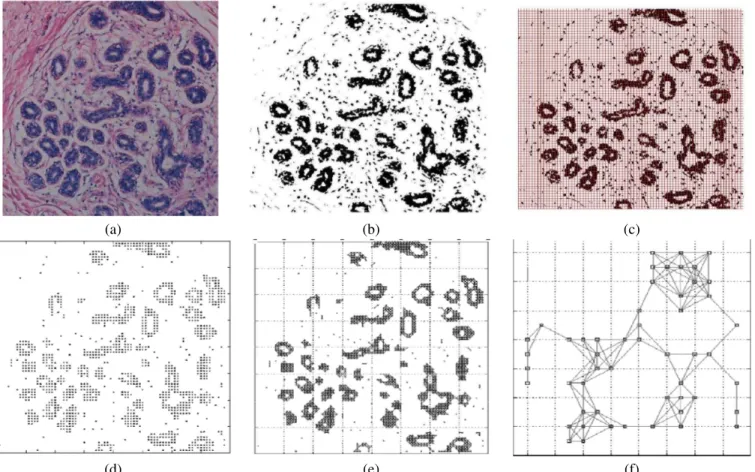
(a) (b) (c)

(d) (e) (f)

Fig. 2. The steps of our methodology. (a) Original tissue image is opened in RGB space. (b) The result of k-means segmentation. (c) The application of grid and thresholding to the resulting segmentation. (d) The overall result of node identification. (e) Simple cell-graphs are formed based on the location information of the cells. (f) Hierarchical graphs are build on cluster cells.

by breast pathologist Dr. Nagi in collaboration with Shabnam Jaffer MD. at MSSM to reach a consensus.

Three major diagnostic groups are formed and analyzed for data preparation. The first group consists of normal breast tissues which are obtained from surgical pathology material. The second group consists of benign reactive processes, such as hyperplasia, radial scar or inflammatory changes. Florid hyperplasia may simulate duct carcinoma in situ based on cellularity. However, histopathologically they are usually easily discernable from neoplasms. The rationale for including this category is to test that high cellularity alone is not mistaken for a neoplastic process using the model that is proposed. Other benign conditions such as sclerosing adenosis is also included to ensure that a low power pattern is not confused with invasive carcinoma. The third major diagnostic group is infiltrating carcinomas. The definition and grading of these tumors is performed according to the published guidelines of the modified Bloom Richardson criteria.

Our data set contains images of 446 breast tissue samples that are removed from 36 different patients. We split this data set into the training and test sets each of having 18 patients. The patients of the training and test sets are disjoint. In the training set, we use 84 invasive cancerous tissue images of 10 patients, 38 non-invasive cancerous tissue images of 5 patients, and 82 benign tissue images of 10 patients. In the test set, the distribution is: 118 invasive cancerous tissue

images of 9 patients, 55 DCIS tissue images of 6 patients, and 69 benign tissue images of 9 patients.

B. Results and Interpretation

We have calculated the accuracy of intensity-based ap-proach, Delaunay-based approach [13], [14], simple cell-graphs, hierarchical cell-graphs and hybrid-based approach and then compared them to each other in table III.

Intensity-based learning: In [11] using gray-level

his-tograms, the sum and mean of the optical densities of the pixels located in a nucleus are defined and computed. Likewise we extracted intensity-based features by employing the RGB values of pixels in a tissue. For each color channel, we computed the mean, standard deviation, skewness and kurtosis of the pixel values of an image and used them as the feature set of our learning algorithm.

From table III we see that intensity-based approach achieves a learning ratio of 61.0%. Delaunay triangulation of the cells produces worse results than the intensity-based approach even though this triangulation embeds the spatial distribution of the cells. Simple cell-graphs, however, embeds the spatial distribution of the cells better than the Delaunay triangulation and achieve a 75.93%±2.53 learning ratio on average for link thresholds varying between 1 and 10. Prob-abilistic cell-graphs do not change the results significantly compared to simple cell-graphs and achieve a learning ratio of 73.4%±1.24.

TABLE I PROBABILISTICCELL-GRAPHS Link 5 6 7 8 9 Threshold Benign 92.0±3 88.7±4 89.2±4 91.6±2 91.1±3 In-Situ 50.9±4 54.9±6 55.1±5 50.2±4 47.8±7 Invasive 79.2±4 75.9±4 74.6±7 77.1±4 78.1±3 Overall 74.5±2 73.2±3 72.6±4 73.1±1 72.9±2 TABLE II

HIERARCHICALCELL-GRAPHRESULTS

Grid Link Threshold

Size 1 2 3 4 5 6 7 8 9 4 60.1 67.0 59.6 57.6 68.5 61.6 64.0 60.6 58.6 5 64.3 66.0 70.0 60.6 66.5 60.6 58.6 71.4 57.6 8 68.9 65.0 73.9 74.9 70.4 65.0 64.0 63.1 63.5 10 76.4 81.8 75.9 70.0 69.5 70.4 66.0 66.0 66.0 16 69.5 68.0 70.0 69.5 69.5 69.5 69.5 69.5 69.5 TABLE III

COMPARISON OF THE TECHNIQUES

Inten. Delaun. Prob. Simple Hier. Hybrid Benign 85.3 80.9 90.5 84.7 82.9 90.9 In-Situ 50.9 16.3 51.8 51.6 75.6 57.3 Invasive 51.7 56.7 77.0 85.6 83.3 86.3 Overall 61.0 54.1 73.4 75.8 81.8 79.1 TABLE IV DETAILEDCOMPARISONS

Intensity Delaunay Hierarchical

Prediction Prediction Prediction

Act Ben InS Inv Ben InS Inv Ben InS Inv

Ben 85.3 10.3 4.4 80.9 10.3 8.8 82.9 7.3 9.8

InS 16.4 50.9 32.7 49.1 16.4 34.5 5.5 75.6 18.9 Inv 14.4 33.9 51.7 27.1 16.1 56.8 8.3 8.3 83.3

Choosing a good parameter set is crucial for the accuracy. Table I shows the accuracy of the classifier with varying link values for probabilistic cell-graphs. We run our probabilistic algorithms for 15 times to get a good estimate of the accu-racy. For hierarchical graphs a good choice of the metrics is small link threshold and a fairly big grid size to find the clusters. For these graphs, after some point increasing the link threshold does not change the learning ratio as can be seen in table II. This is because we obtain a complete graph where each node has a link to the other nodes. A grid size of 10 is able to capture the cell clusters and obtains a learning ratio of 81.8%.

In hybrid-based approach we have combined the intensity features, the metrics calculated from simple cell-graphs and hierarchical cell-graphs and used this set as the feature set of our classifier. This hybrid approach is calculated for a grid size of 10 and the average value for this technique is 79.1%. The over all learning ratios in table III suggest that hier-archical cell-graphs perform better than the other techniques presented in this paper. Besides, the learning ratio for in-situ case is 75.6% using hierarchical graphs and the closest result to this is 57.3% using hybrid approach. In table IV where Ben, InS, Inv and Act stands for benign, in-situ, invasive, and actual (true) class, we have also presented the confusion matrices of the techniques. We see that hierarchical cell-graphs have false positive and false negative values smaller than 10%.

V. CONCLUSION

Cell-graphs enable us to identify and compute a rich set of features that represent the structure of breast tissues. These feature sets are input to a SVM for classification of benign, invasive and noninvasive cancerous tissues. Previously, we presented cell-graphs for brain tissue samples which present a diffusive structure. In this work we extend and enhance the cell-graph approach to model and classify breast tissue samples which has a lobular/glandular architecture, thus dif-fer from brain tissues significantly in architecture. To capture this difference we introduce hierarchical graphs and obtain an accuracy of 81.8%. Our technnique has false-positive and false-negative values less than 10%. We also give a computational comparison of our approach to the related work in the literature shows that hierarchical cell-graphs are much more accurate for breast tissues. However, we believe that accuracy can be improved further by increasing the data size and by improving the image segmentation.

REFERENCES

[1] A.G. Todman, R.N.G. Naguib, and M.K. Bennett, ”Orientational Coherence Metrics: Classification of Colonic Cancer Images Based on Human Form Perception”, Proc. Canadian Conf. Electrical and

Computer Eng, vol. 2, 2001, pp. 1379-1384,

[2] A.N. Esgiar, R.N.G. Naguib, B.S. Sharif, M.K. Bennett and A. Murray, ”Fractal Analysis in the Detection of Colonic Cancer Images”, IEEE

Trans. Inf. Tech. in Biomedicine, vol. 6, no. 1, 2002, pp. 54-58.

[3] D. Glotsos, P. Spyridonos, P. Petalas, G. Nikiforidis, D. Cavouras, P. Ravazoula, P. Dadioti, and I. Lekka, ”Support Vector Machines for Classification of Histopathological Images of Brain Tumour Astrocy-tomas”, Proc. Intl Conf. Computational Methods in Sciences and Eng., 2003 pp. 192-195.

[4] F. Schnorrenberg, C.S. Pattichis, C.N. Schizas, K. Kyriacou, and M.Vassiliou ”Computer-Aided Classification of Breast Cancer Nuclei”,

Technology and Health Care, vol. 4, no. 2, 1996, pp. 147-161.

[5] C. Gunduz, B. Yener, and S. H. Gultekin, ”The cell graphs of cancer”,

Bioinformatics, vol. 20 2004, i145-i151.

[6] I. Guyon, Weston,J., Barnhill,S. and Vapnik,V. Gene selection for can-cer classification using support vector machines, Machine Learning, 46, 2002, 389422.

[7] H. Ganster, P. Pinz, R. Rohrer, E. Wildling, M. Binder, and H.Kittler, ”Automated Melanoma Recognition (2001)”, IEEE Trans. Medical

Imaging, vol. 20, no. 3, 2001, pp. 233-239.

[8] H. Jeong, Tombor, R. Albert, Z. N. Oltvai, A.-L. Barabasi, ”The large-scale organization of metabolic networks”, Nature vol. 407, 2000, pp. 651-654.

[9] P.W. Hamilton, D.C. Allen, P.C. Watt, C.C Patterson, and J.D. Biggart, ”Classification of Normal Colorectal Mucosa and Adenocarcinoma by Morphometry”, Histopathology, vol. 11, no. 9, 1987, pp. 901-911. [10] R. Rifkin, S. Mukherjee, P. Tamayo, S. Ramaswamy, C.-H. Yeang,

M. Angelo, M. Reich, T. Poggio, E.S. Lander, T.R. Golub, and J.P. Mesirov, ”An analytical method for multiclass molecular cancer classification”, SIAM Rev, 45, 2003, 706723.

[11] B. Weyn, G. Van de Wouwer, S. Kumar-Singh, A. Van Daele, P. Scheunders, E. Van Marck, and W. Jacob, ”Computer-assisted differen-tial diagnosis of malignant mesothelioma based on syntactic structure analysis”, Cytometry, vol. 35, 1999, pp. 23-29.

[12] B. Wu, T. Abbott, D. Fishman, W. McMurray, G. Mor, K. Stone, D. Ward, K. Williams, and H. Zhao, ”Comparison of statistical methods for classification of ovarian cancer using mass spectrometry data”,

Bioinformatics, 19, 2003, pp. 16361643.

[13] S. Keenan, J. Diamond, W.G. McCluggage, H. Bharucha, D. Thomp-son, B.H. Bartels, P.W. Hamilton, ”An automated machine vision system for the histological grading of cervical intraepithelial neoplasia (CIN)”, Journal of Patholology, vol. 192, 2000, pp. 351-362. [14] H. Choi, T. Jarkrans, E. Bengtsson, J. Vasko, K. Wester, P. Malmstrom,

C. Busch, ”Image analysis based grading of bladder carcinoma. Comparison of object, texture and graph based methods and their reproducibility”, Analytical Cellular Pathology, 15, 1997, pp. 1-18.