LOCALITY AWARE REORDERING FOR
SPARSE TRIANGULAR SOLVE
a thesis
submitted to the department of computer engineering
and the graduate school of engineering and science
of bilkent university
in partial fulfillment of the requirements
for the degree of
master of science
By
Tu˘
gba Torun
September, 2014
I certify that I have read this thesis and that in my opinion it is fully adequate, in scope and in quality, as a thesis for the degree of Master of Science.
Prof. Dr. Cevdet Aykanat (Advisor)
I certify that I have read this thesis and that in my opinion it is fully adequate, in scope and in quality, as a thesis for the degree of Master of Science.
Prof. Dr. U˘gur G¨ud¨ukbay
I certify that I have read this thesis and that in my opinion it is fully adequate, in scope and in quality, as a thesis for the degree of Master of Science.
Assoc. Prof. Dr. Oya Ekin Kara¸san
Approved for the Graduate School of Engineering and Science:
Prof. Dr. Levent Onural Director of the Graduate School
ABSTRACT
LOCALITY AWARE REORDERING FOR SPARSE
TRIANGULAR SOLVE
Tu˘gba Torun
M.S. in Computer Engineering Supervisor: Prof. Dr. Cevdet Aykanat
September, 2014
Sparse Triangular Solve (SpTS) is a commonly used kernel in a wide variety of scientific and engineering applications. Efficient implementation of this kernel on current architectures that involve deep cache hierarchy is crucial for attaining high performance. In this work, we propose an effective framework for cache-aware SpTS.
Solution of sparse linear symmetric systems utilizing the direct methods re-quire the triangular solve of the form LU z = b, where L is lower triangular factor and U is upper triangular factor. For cache utilization, we reorder the rows and columns of the L factor regarding the data dependencies of the triangular solve. We represent the data dependencies of the triangular solve as a directed hyper-graph and construct an ordered partitioning model on this structure. For this purpose, we developed a variant of Fiduccia-Mattheyses (FM) algorithm which respects the dependency constraints. We also adopt the idea of splitting L fac-tors into dense and sparse components and solving them seperately with different autotuned kernels for achieving more flexibility in this process. We investigate the performance variation of different storage schemes of L factors and the cor-responding sparse and dense components. We utilize autotuning provided by Optimized Sparse Kernel Interface (OSKI) to reduce performance degradation that incurs due to the gap between processors and memory speeds. Experiments performed on real-world datasets verify the effectiveness of the proposed frame-work.
Keywords: Sparse matrices, triangular solve, cache locality, matrix reordering, hypergraph partitioning, directed hypergraph.
¨
OZET
SEYREK ¨
UC
¸ GENSEL S˙ISTEMLER˙IN ¨
ONBELLEK
YERELL˙I ˘
G˙INE G ¨
ORE YEN˙IDEN SIRALANMASI
Tu˘gba TorunBilgisayar M¨uhendisli˘gi, Y¨uksek Lisans Tez Y¨oneticisi: Prof. Dr. Cevdet Aykanat
Eyl¨ul, 2014
Seyrek ¨u¸cgensel sistem ¸c¨oz¨um¨u, bir ¸cok bilimsel ve m¨uhendislik uygulamalarında yaygın olarak kullanılan bir ¸cekirdek i¸slemdir. Bu ¸cekirdek i¸slemin ¸cok seviyeli ¨
onbellekler ¨uzerinde etkili bir ¸sekilde y¨ur¨ut¨ulmesi, y¨uksek permormans elde et-mek a¸cısından ¨onemlidir. Biz bu ¸calı¸smada, seyrek ¨u¸cgensel sistem ¸c¨oz¨um¨unde kullanılmak ¨uzere etkili bir ¸cer¸ceve sunuyoruz.
Seyrek lineer sistemlerin direkt metod ile ¸c¨oz¨um¨u, L alt ¨u¸cgensel fakt¨or ve U ¨ust ¨u¸cgensel fakt¨or olmak ¨uzere, LU z = b bi¸cimindeki bir ¨u¸cgensel den-klem ¸c¨oz¨um¨un¨u gerektirir. Onbelle˘¨ gi kullanmak i¸cin, ¨u¸cgensel sistemdeki veri ba˘glılı˘gını da g¨oz ¨on¨une alarak L fakt¨or¨un¨un satır ve s¨utunlarını yeniden sıraladık.
¨
U¸cgensel sistemdeki veri ba˘glılıklarını y¨onl¨u bir hiper¸cizge olarak kodlayıp, bu yapı ¨uzerinde sıralı bir b¨ol¨umleme modeli in¸sa ettik. Bu ama¸cla, ba˘glılık sınırlamalarına riayet edecek bi¸cimde Fiduccia-Mattheyses (FM) algoritmasını farklı bir ¸sekilde yeniden geli¸stirdik. Ayrıca, bu i¸slemde daha fazla esneklik elde etmek i¸cin, L fakt¨orlerini seyrek ve yo˘gun par¸calara ayırma fikrini benimsedik ve her bir par¸cayı otomatik ayarlanmı¸s farklı ¸cekirdek y¨ontemlerle ¸c¨ozd¨uk. Farklı depolama y¨ontemleri kullanarak L fakt¨or¨un¨un ve buna kar¸sılık gelen seyrek ve yo˘gun par¸caların performans de˘gi¸simini inceledik. ˙I¸slemci ve hafıza arasındaki hız farklarından kaynaklanan performans kayıplarını ¨onlemek i¸cin, OSKI tarafından sa˘glanan otomatik ayarlama y¨ontemlerinden faydalandık. Ger¸cek veriler ¨uzerinde y¨ur¨ut¨ulen deneyler, ¨onerilen modelin etkinli˘gini do˘grular niteliktedir.
Anahtar s¨ozc¨ukler : Seyrek matrisler, ¨u¸cgensel sistemler, ¨onbellek yerelli˘gi, matrisi yeniden sıralama, hiper¸cizge b¨ol¨umleme, y¨onl¨u hiper¸cizge .
Acknowledgement
I would like to thank my supervisor Prof. Dr. Cevdet Aykanat for his valuable advices, suggestions and assistence throughout the development of this thesis.
I owe thanks to Prof. Dr. U˘gur G¨ud¨ukbay and Assoc. Prof. Dr. Oya Ekin Kara¸san for spending their time to evaluate and comment on the thesis. I also thank Kadir Akbudak for his helps and contributions for the progress of this study.
I am grateful to my family for their infinite moral support and help. My special thank goes to my husband F. S¸¨ukr¨u Torun for his endless support, encouragement and patience all along my studies. He deserves the best I can give for facilitating and beautifying my life.
Finally, I thank T ¨UB˙ITAK for the supporting grant supplied throughout my master program.
Contents
1 Introduction 1
2 Background 4
2.1 Direct Method for Solving Linear Systems . . . 4
2.1.1 Forward Substitution . . . 6
2.1.2 Backward Substitution . . . 8
2.2 Graph Partitioning . . . 9
2.3 Hypergraph Partitioning . . . 10
2.4 Directed Graph Representation for Dependencies in Forward Sub-stitution . . . 12
2.5 Sparse Matrix Storage Schemes . . . 14
2.5.1 Compressed Storage Formats . . . 14
2.5.2 Block Compressed Storage Formats . . . 14
2.6 Data Locality in Forward Substitution . . . 15
CONTENTS viii
2.8 Exploiting Cache Locality in SpMxV . . . 17
3 Related Work 19 4 Directed Hypergraph Partitioning Model for Cache Aware For-ward Substitution 21 4.1 Reordering Triangular Matrix For Exploiting Cache Locality . . . 21
4.2 Deficiencies of Directed Graph Partitioning Model for Reordering Triangular Matrices . . . 26
4.3 Directed Hypergraph Representation of Forward Substitution . . . 27
4.4 Directed Hypergraph Partitioning (dHP) . . . 30
4.4.1 Recursive Bipartitioning . . . 33
4.4.2 Directed Fiduccia-Mattheyses (dFM) Algorithm . . . 35
4.4.3 Clustering in dHP . . . 38 5 Experimental Results 40 5.1 Experimental Setup . . . 40 5.2 Datasets . . . 42 5.3 Results . . . 45 6 Conclusion 58
List of Figures
2.1 Directed dependence graph representation for row/ column ori-ented forward substitution . . . 13
4.1 Reordering rows of lower triangular factor L for exploiting tempo-ral locality in row-oriented forward substitution . . . 22 4.2 Reordering columns of lower triangular factor L for exploiting
tem-poral locality in column-oriented forward substitution . . . 23 4.3 Reordering rows/columns without obeying dependency rules would
destroy lower-triangularity . . . 24 4.4 Partitioning the L factor and corresponding dependence graph . . 26 4.5 Column-net directed hypergraph representation of forward
substi-tution . . . 29 4.6 Row-net directed hypergraph representation of forward substitution 30 4.7 Rowwise partitioning the L factor and the corresponding
column-net directed hypergraph . . . 32
A.1 Original matrix bcsstk17 . . . 65 A.2 L factor of matrix bcsstk17 obtained by Cholesky Factorization . 66
LIST OF FIGURES x
A.3 L factor of matrix bcsstk17 after reordering with row-wise dHP . 67 A.4 L1 part of matrix bcsstk17 . . . 68
A.5 L1 part of matrix bcsstk17 after reordering with row-wise dHP . 69
A.6 L11 part of matrix bcsstk17 . . . 70
List of Tables
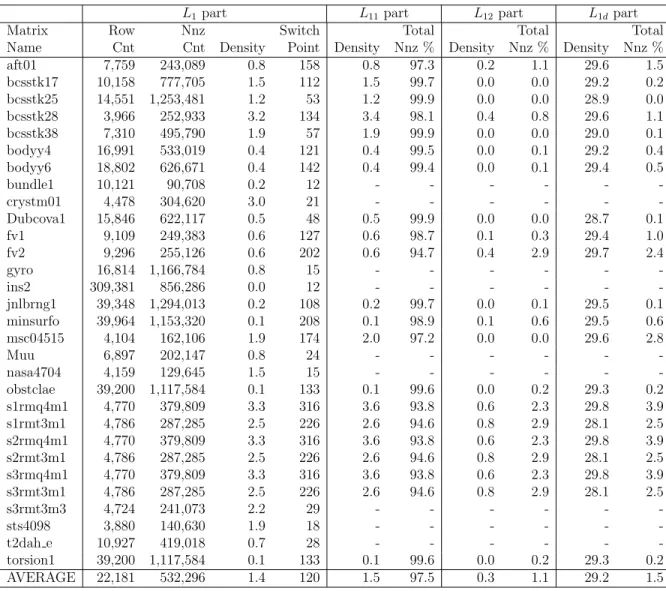
5.1 Sparsities of submatrices obtained by 1. splitting . . . 43
5.2 Sparsities of submatrices obtained by 2. splitting . . . 44
5.3 Cutsize reduction by directed hypergraph partitioning on L factors 46 5.4 Cutsize reduction by directed hypergraph partitioning on L1 part 47 5.5 Cutsize reduction by directed hypergraph partitioning on L11 part 48 5.6 Runtime improvement of dHP model on L factor . . . 50
5.7 Runtime improvement of dHP model on L1 part . . . 51
5.8 Runtime improvement of dHP model on L11 part . . . 52
5.9 Runtime improvement of dHP by 1. splitting . . . 54
5.10 Runtime improvement of dHP by 2. splitting . . . 55
Chapter 1
Introduction
Developments in computer architectures bring along the performance gap between the processor and memory speeds. This gap becomes more critical due to the hierarchical memory structure. Yet it can be reduced by exploiting high level memory units (caches) efficiently, which are faster but smaller memories compared to RAM. Hence extra attention is needed for the applications whose performance highly depends on memory utilization.
Data localities can be exploited if the data is accessed in consecutive mem-ory localitions. An application is called regular if it enables such utilizations of data localities and called irregular , otherwise. Utilizing data locality in irregu-lar computations is a challenging task due to the irreguirregu-larity in memory access patterns.
Sparse Triangular Solve (SpTS) is an instance of such an irregular computation and it is one of the most important kernels in numerical computing. It arises in several scientific and engineering applications including direct solution of sparse linear systems, preconditioning of iterative methods and least squares problems [1, 2, 3]. It requires to solve the sparse triangular system of the form T x = b with respect to dense solution vector x, given a sparse triangular matrix T and dense vector b.
The performance of SpTS is directly effected by the sparsity pattern of the triangular matrix. The data localities in SpTS can be utilized when the nonzeros of triangular matrix stay close to each other. However in most of the real-world applications, the nonzero distributions and hence the memory access patterns are irregular, which yields a poor utilization of cache. Nevertheless, altering the nonzero distribution to obtain more regular patterns is possible by applying proper reordering methods.
In literature, the method of reordering rows/ columns of matrices for cache utilization has been frequently exploited in applications like sparse matrix-vector multiplication (SpMxV) [4, 5, 6]. However, these reordering techniques has not been adressed for cache utilization in SpTS to the best of our knowlegde. The main reason for this case might be the low flexibility in SpTS due to high depen-dencies between computations unlike other applications: Solution of SpTS include computations which may depend on others, according to the nonzero distribution in triangular solve. Hence these order of computations must be protected while reordering the rows/ columns associated with the corresponding computations.
In this thesis, we investigate a reordering method on the rows and columns of the triangular matrix for better cache utilization, by taking the data dependen-cies into account. To obtain such a reordering, we represent dependendependen-cies among the computations of SpTS as a directed hypergraph. We develop a novel ordered partitioning model upon this directed hypergraph representation. We argue that cutsize reduction in this directed hypergraph partitioning (dHP) model corre-sponds to minimizing cache misses in SpTS. We extend the Fiduccia-Mattheyses (FM) algorithm [7] with more feasibility restrictions and updates in order to cap-ture the ordered-directed struccap-ture of the required partitioning model. The rows and the columns of the triangular factor is reaordered symmetrically according to the final order of vertices obtained by the dHP model.
Based upon this reordering model, we propose a framework for efficient cache utilization in SpTS. We exploit the idea of splitting the triangular matrix into dense and sparse parts proposed by [8] in order to obtain higher flexibilities for our dHP model. By this way the SpTS problem is converted into solving a
sub-SpTS, a SpMxV and a dense triangular solve. We utilize our dHP model for solving this smaller SpTS which shows a more flexible charecteristic than the original SpTS in terms of having fewer data dependencies and the ease of reordering. We also apply the hypergraph-partitioning based reordering method of rectangular matrices proposed in [6] for cache utilization in SpMxV in order to enhance the overall SpTS performance. The autotuning provided by OSKI library [9] is exploited to utilize higher levels of memory more effectively.
The rest of the thesis is organized as follows: Necessary background material for this study is provided in Chapter 2. In Chapter 3, we review the previous works which are most relevant to our framework. The directed hypergraph par-titioning model is introduced and demonstrated in Chapter 4. We present the experimental results in Chapter 5 and conclude the thesis in Chapter 6.
Chapter 2
Background
2.1
Direct Method for Solving Linear Systems
Most of the scientific computing problems requires the solution of a linear sys-tem. Linear systems are used in linear programming, discretization of nonlinear systems and differential equations. In a linear system of the form
Az = b, (2.1)
the aim is to find the column vector z , with a given coefficient matrix A and a column vector b. There are two classes of methods for solving systems of linear equations: Direct methods and iterative methods.
In iterative methods, beginning with an initial approximation, a sequence of approximate solutions is computed until a desired accuracy is obtained [10]. On the other hand, in direct methods, the solution is obtained in a finite number of operations. In these methods, the coefficient matrix of the linear system is transformed or factorized into a simpler form which can be solved easier. Direct methods have been preferred over iterative methods for solving linear systems mainly because of their stability and robustness [11].
into its lower triangular factor L and upper triangular factor U as
A = LU. (2.2)
A lower triangular matrix is a square matrix whose all of the nonzero entries lie below and on the main diagonal. Similarly, an upper triangular matrix is a square matrix which has all of its nonzero entries above and on the main diagonal. A square matrix which is either lower triangular or upper triangular is referred to as a triangular matrix.
The diagonal entries of the triangular factors should be nonzero in order to avoid round-off errors in the upcoming operations of direct method. For this reason, permuting the rows and columns of the coefficient matrix is allowed in the LU factorization. This procedure is called pivoting and there are two ways to do it: Partial pivoting reorders the rows of the coefficient matrix during the LU factorization in order to move the entry with maximum absolute value of a column to the diagonal. In complete pivoting, both the rows and the columns can be permuted in order to make the diagonal entry to have the largest absolute value in the entire remaining unprocessed submatrix. This procedure enhances the numerical stability.
In particular, if the coefficient matrix A is symmetric and positive definitive (having all eigenvalues positive), the diagonal elements of L and U factors become nonzero without requiring any pivoting. Furthermore in this case there exist a unique factorization, namely Cholesky factorization, such that U = LT holds in
Equation (2.2).
After obtaining the triangular factors, the Equation (2.2) is substituted into the original linear system Equation (2.1) and the problem becomes
LU z = b, (2.3)
which is equivalent to solving the following set of two equations:
Lx = b, (2.4)
Here, Equation (2.4) is solved with a procedure called forward substitution and Equation (2.5) is solved with backward substitution. First the forward substitution (2.4) is solved to find x vector, and then the x vector is substituted in the backward substitution Equation (2.5) to get the z vector.
2.1.1
Forward Substitution
Let us assume that L = (li,j)0≤i,j≤n is a lower triangular matrix. Note that by
the definition of lower triangularity, li,j = 0 whenever i < j . Then the
lower-triangular system Lx = b with x = (xi)0≤i≤n and b = (bi)0≤i≤n
l1,1 l2,1 l2,2 . .. ln,1 ln,2 · · · ln,n · x1 x2 .. . xn = b1 b2 .. . bn
is equivalent to the following system of equations:
l1,1x1 = b1 l2,1x1+ l2,2x2 = b2 l3,1x1+ l3,2x2+ l3,3x3 = b3 .. . ln−1,1x1+ ln−1,2x2+ · · · + ln−1,n−1xn−1 = bn−1 ln,1x1+ ln,2x2+ · · · + ln,n−1xn−1+ ln,nxn= bn (2.6)
By these equations, the x vector can be solved by computing xi entries from
x1 = b1 l1,1 x2 = b2− l2,1x1 l2,2 x3 = b3− l3,2x2− l3,1x1 l3,3 .. . xn = bn− ln,n−1xn−1− · · · − ln,2x2− ln,1x1 ln,n (2.7)
Forward substitution method finds the xi entries in the increasing order of the
indices: x1 is computed first and then substituted forward into the next equation
for solving x2, and this process goes on until xn.
There are two popular ways of implementing forward substution: Row-oriented and column-Row-oriented.
2.1.1.1 Row-Oriented Forward Substitution
Row-oriented forward substitution solves Equation (2.7) one row at a time. Firstly, x1 is found from the first equation in (2.7). Then x2 is calculated by
substituting x1 in the second equation of (2.7). Similarly, x3 is obtained by
substituting the values x1 and x2 in the third equation of (2.7) and this
pro-cess is continued until the last equation to get xn. Algorithm 1 represents the
pseudocode of row-oriented forward substitution. Algorithm 1 Row-oriented forward substitution
1: for i ← 1 to n do 2: xi ← bi 3: for j ← 1 to i − 1 do 4: xi ← xi− li,j× xj 5: xi ← xi li,i
2.1.1.2 Column-Oriented Forward Substitution
Column-oriented forward substitution computes Equation (2.7) one column at a time. For i > j , the li,jxj value is subtracted from xi immediately after
computing xj, rather than doing all substractions at the computation time of
xi as in the row-oriented substitution. Algorithm 2 shows the pseudocode of
column-oriented forward substitution.
Algorithm 2 Column-oriented forward substitution
1: for j ← 1 to n do 2: xj ← bj 3: xj ← xj lj,j 4: for i ← j + 1 to n do 5: xi ← xi− li,j× xj
2.1.2
Backward Substitution
Let us assume that U = (ui,j)0≤i,j≤n is an upper triangular matrix. Note that
by the definition of upper triangularity, ui,j = 0 whenever i > j . Then the
upper-triangular system U z = x with z = (zi)0≤i≤n and x = (xi)0≤i≤n
u1,1 u1,2 · · · u1,n u2,2 · · · u2,n . .. un,n · z1 z2 .. . zn = x1 x2 .. . xn
u1,1z1+ u1,2z2+ u1,3z3+ · · · + u1,nzn= x1 u2,2z2+ u2,3z3+ · · · + u2,nzn= x2 .. . un−1,n−1zn−1+ un−1,nzn= xn−1 un,nzn= xn (2.8)
By these equations, the x vector can be solved by computing xi entries from
the following equations in order:
zn= xn un,n zn−1= xn−1− u2,1z1 un−1,n−1 .. . z1 = x1− u1,2z2− u1,3z3− · · · − u1,nzn u1,1 (2.9)
Backward substitution method finds the zi entries in the decreasing order of
the indices: It first computes zn, then substitute it back into the next equation
to find zn−1, and continue backwards until z1.
In this thesis, we will focus on forward substitution since the backward sub-stitution is the reverse of forward subsub-stitution and the proposed models and methods can be applied analogously without loss of generality.
2.2
Graph Partitioning
A graph G = (V, E ) is a representation consisting of a set of vertices V and a set of edges E . Each edge eij connects two distinct vertices vi and vj. Each vertex
also have directions associated with them. Directed edges are ordered pairs of vertices.
Given a graph G = (V, E ), Π = {V1, . . . , VK} is called a K -way partition of
the vertex set V if each part Vk contains at least one vertex, the intersection of
two distinct parts is empty, and the union of all parts is equal to V . Specifically, a K -way partition is called a bipartition if K = 2.
The sum of the weights of the vertices in part Pk is called the weight of that
part and denoted as Wk. A K -way partition of G is said to satisfy the balance
criteria and be balanced if
Wk≤ (1 + ε)Wavg, for k = 1, 2, . . . , K (2.10)
where ε is a predetermined, maximum allowable imbalance ratio and Wavg is the
average part weight, i.e. Wavg= (
P
1≤k≤KWk)/K .
An edge is called cut (external) if it connects two vertices from different parts, and called uncut (internal) otherwise. Let the set of cut edges is represented by Ecut. Then the cutsize of a partition Π is defined as the sum of the costs of cut
edges:
cutsize(Π) = X
eij∈Ecut
c(eij). (2.11)
The graph partitioning problem is to partition the graph into K disjoint parts with minimum cutsize, while satisfying the balanca criteria 2.10. This problem is known to be NP-hard even for unweighted graph bipartitioning [12].
2.3
Hypergraph Partitioning
Hypergraphs are generalization of graphs in which each hyperedge can connect more than two vertices as opposed to the edges in graphs connecting only two vertices. A hypergraph H = (V, N ) consists of a set of vertices V and a set of hyperedges (nets) N . Each net nj ∈ N connects an arbitrary subset of vertices,
represented by P ins(nj). The set of nets connected to a vertex vi is represented
by N ets(vi). The weight of vertex vi ∈ V and the cost of the net nj ∈ N are
denoted as w(vi) and c(nj), respectively.
The definitions of K -way partition and balance criteria for the graph parti-tioning hold for hypergraphs as well. For a partition Π of H , if a net connects at least one pin in a part, then that net is said to connect that part. The set of parts connected by a net nj is called the connectivity set Λj of nj. The number
of parts connected by a net nj is called the connectivity of nj and denoted by
λj = |Λj|. If a net nj connects more than one part (i.e., λj > 1), then it is
said to be a cut (external ) net, and otherwise (i.e., λj = 1) it is called an uncut
(internal ) net. The cutsize of a partition Π is defined as
cutsize(Π) = X
nj∈NE
(λj− 1), (2.12)
in which each cut net nj contributes λj − 1 to the cutsize. The partitioning
objective is to minimize the cutsize while maintaining the balance criteria (2.10). The hypergraph partitioning problem is also known to be NP-hard [13].
For K -way hypergraph partitioning, a paradigm called recursive bisection is widely used [14, 15]. In this paradigm, the hypergraph is bipartitioned into two parts initially. Then each part of this bipartition is further bipartitioned recursively until a predetermined part count K is obtained or the weight of a part drops below a predetermined maximum part weight value. This paradigm is especially preferred for hypergraph partitioning if the number of parts is not known in advance.
Most of the hypergraph bipartitioning algorithms relies on Fiduccia-Mattheyses (FM) [7] and Kernighan-Lin (KL) [16] heuristics which were proposed for reducing the cutsize of a bipartition. KL-based heuristics swap two vertices from different parts of the bipartition while FM-based heuristics move a single vertex from one part to the other.
of moving a vertex to other part is called the gain of that vertex. The gains of vertices can be stored in buckets or heaps [17, 18]. The FM heuristic consists of multiple passes each of which begins with unlocked vertices. At each step of a pass, the vertex with the highest gain value is selected, moved to the other part and locked. After each move, the gain values of the unlocked neighbors of the moved vertex are updated and the improvement in the cutsize is stored. A pass terminates if all vertices become locked or no feasible move reamins. At the end of each pass, the partition which gives the minimum cutsize is restored. Several passes are performed until the reduction in the cutsize drops below a predetermined threshold.
The hypergraph partitioning model is widely used to represent and partition sparse matrices [19]. Mainly there are two hypergraph models proposed for sparse matrix partitioning, namely row-net and column-net models [20, 21]. In row-net hypergraph model, the nets represents the rows of a matrix and the vertices rep-resent the columns of the matrix whereas in the column-net model, nets reprep-resent the columns and vertices represent the rows.
2.4
Directed Graph Representation for
Depen-dencies in Forward Substitution
In a forward substitution with dense L matrix, the computation order of xi
entries should be exactly the same as the order in (2.7). The reason is that all the xj entries with j < i should be computed beforehand for substituting the
li,jxj value in the computation equation of xi entry. For a sparse L matrix, on
the other hand, the computation of xi does not depend on xj (j < i) if the li,j
entry of the L matrix is zero, since then the li,jxj value will be automatically
zero and will not be used in the computation of xi. Yet the computation of xi
should still wait the value of xj (j < i) if the li,j entry is a nonzero.
In other words, the ith equation of (2.7) can not be solved before the jth
can not be processed before row j if li,j 6= 0 (j < i). Row i is said to depend on
row j if li,j 6= 0 with j < i. Conversely, if li,j = 0 with j < i, then row i is said
to be independent from row j .
Similarly for column-oriented forward substitution, column i can not be pro-cessed before column j if li,j 6= 0 (j < i). This dependency is expressed in terms
of the columns of the matrix as follows: Column i is said to depend on column j if li,j 6= 0 and said to be independent from column j if li,j = 0 for j < i.
These dependencies can also be converted to a directed graph representa-tion. According to the data dependencies in row-oriented forward substitution, a directed dependence graph is constructed corresponding to the lower triangu-lar factor L such that vertex vi represents row i and there is a directed edge
eji from vertex j to i whenever li,j 6= 0 (j < i). Theoretically speaking, for
column-oriented forward substitution, vertex vi represents column i but the edge
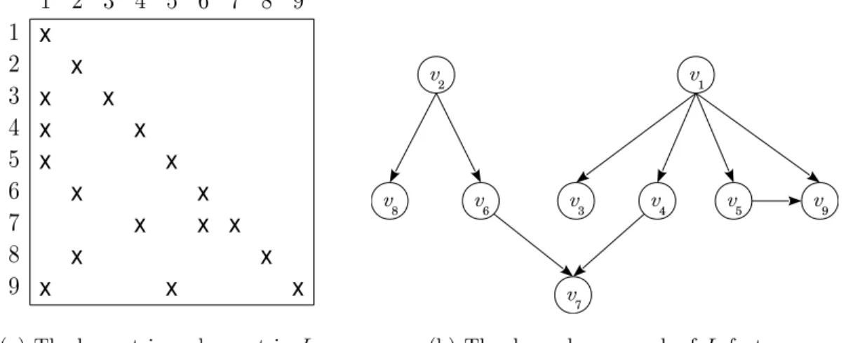
definitions are the same and so the corresponding dependence graph is equivalent. Figure 2.1(a) illustrates a sample lower triangular factor L of size 9 × 9. In Figure 2.1(b), the corresponding dependence graph of L factor is constructed. Directed edges e13, e14, e15, e19, e26, e28, e47, e59, e67 correspond to the nonzero
entries l3,1, l4,1, l5,1, l9,1, l6,2, l8,2, l7,4, l9,5, l7,6 of the L factor respectively.
(a) The lower triangular matrix L (b) The dependence graph of L factor
Figure 2.1: Directed dependence graph representation for row/ column oriented forward substitution
2.5
Sparse Matrix Storage Schemes
We will beriefly describe the compressed storage formats which are the most common sparse matrix storage schemes, and a variant of this format, namely the block compressed storage format, which improves the performance in most of the sparse matrix operations.
2.5.1
Compressed Storage Formats
Sparse matrices are often stored in a compressed format in which only the nonze-ros of the sparse matrices and their localitions are stored. Mainly, each nonzero element of the matrix is stored into a linear array and some additional arrays are provided to describe the locations of the nonzeros in the matrix. This format is frequently preferred for sparse matrices since it does not store any unnecessary information about the zero elements that dominate the sparse matrices [22, 23].
There are two main compressed storage schemes, namely Compressed Storage by Rows (CSR) and Compressed Storage by Columns (CSC). CSR scheme stores the nonzeros in a row-major format, i.e. stores the nonzeros of a row consecutively while CSC scheme stores the nonzeros in a column-major format, i.e., stores the nonzeros of columns consecutively.
2.5.2
Block Compressed Storage Formats
Block Compressed Storage by Rows (BSCR) and Block Compressed Storage by Columns (BCSC) are the modified versions of CRS and CCS formats to exploit dense block patterns respectively. The matrix is partitioned into small blocks whose sizes evenly divide the dimensions of the matrix. Each block is treated as a dense matrix even if it has some zeros in these blocks but the blocks consisting of only zero elements are not stored. In BSCR (BCSC) format, the column (row) indices are stored block-by-block and the pointers reference to rows (columns) of blocks.
For arithmetic operations with sparse matrices having dense sub-matrices, us-ing block storage formats is considerably more efficient than usus-ing regular com-pressed sparse storage formats. Especially for matrices with large block dimen-sions, the block compressed storage formats significantly reduce the time spent in performing indirect addressing and the memory requirements for storage locations with respect to the usual compressed storage formats.
Determining the dimensions of dense block patterns which leads to the fastest implementation is referred as tuning . This process should be handled at run-time automatically (which is called autotuning ) for sparse matrices since the best data structure depends on the sparsity pattern of the matrix. The Optimized Sparse Kernel Interface (OSKI) [9] library provides an autotuning framework for SpTS.
2.6
Data Locality in Forward Substitution
Here, we will briefly discuss how data locality can be achieved in the forward substitution Lx = b. The row-oriented forward substitution algorithm puts all of the previously computed entries xj into the equation just before computing
xi where (j < i). On the other hand, the column-oriented forward substitution
algorithm updates xi entry immediately after computing xj for each j < i. These
two algorithms seem to have the same computation order for the x vector entries and the same number of operations, but they process data in different order and hence access memory in different patterns.
There are mainly two ways to exploit cache locality: Temporal and spatial locality. Temporal locality refers to reuse of data which is previously fetched and still staying in the cache. Spatial locality allows reuse of data which was previously prefetched when a data from a nearby location was brought to the cache.
In row-oriented forward substitution, spatial locality in terms of the nonzeros of lower triangular factor can be automatically exploited if it is stored in a row-major (e.g. CSR, BCSR) format. Similarly for column-oriented substitution, we can automatically exploit spatial locality if we store the lower triangular factor
in a column-major (e.g., CSC, BCSC) format. This is because in these cases the nonzero entries of the component matrix stored and processed consecutively. The temporal locality for the nonzeros of lower triangular factor is not feasible since each entry is accessed only once. The same reasons hold to say that the spatial locality is automatically achieved and the temporal locality cannot be exploited in accessing the entries of the b-vector.
The spatial locality in accessing x-vector entries is feasible since the entries are operated consecutively in the case of using a row-major compressed storage format for row-oriented forward substitution and using a column-major compressed stor-age format for column-oriented forward substitution. For row-oriented forward substitution, the temporal locality in accesing x-vector entries is feasible because of the reuse of previously stored data when processing former rows. For column-oriented forward substitution, the temporal locality in accesing x-vector entries is feasible since the previously operated data when processing former columns can be reused. Exploiting temporal locality for x vector is our major concern regarding data locality in sparse triangular solve.
2.7
Splitting Triangular Factor into Dense and
Sparse Parts
We observed that the L factors obtained by Cholesky and LU factorization gen-erally contain a dense submatrix in the lower right-most part of the L factor as mentioned in [8]. This dense part is referred as trailing triangle and accounts for a high fraction of the overall nonzeros. This structure can be exploited by splitting the L factor into sparse and dense components as in [8]. The triangular solve Lx = b is then decomposed as:
" L1 L2 Ld # · " X1 X2 # = " B1 B2 # ,
where L1 is a sparse lower triangular submatrix, L2 is a rectangular sparse
components of x vector (b vector) according to the dimensions of the correspond-ing L factor components. With this decomposition, the triangular solve become equivalent to find the X1 and X2 subvectors by the following set of equations:
L1X1 = B1,
L2X1+ LdX2 = B2,
which can be solved in three steps:
L1X1 = B1, (2.13)
˜
B2 = B2− L2X1, (2.14)
LdX2 = ˜B2. (2.15)
Here, equation 2.13 is a sparse triangular solve where Equation 2.14 is a sparse matrix-vector multiplication (SpMxV) and Equation 2.15 is a dense triangular solve. The process of splitting a lower triangular matrix into dense and sparse parts and solving them seperately can be further proceeded for the L1 part. The
second splitting on L1 part is similarly performed by decomposing L1X1 = B1
as " L11 L12 L1d # · " X11 X12 # = " B11 B12 #
which can be solved in three steps including one sparse triangular solve (SpTS), one sparse matrix vector multiplication (SpMxV) and one dense triangular solve as in the original splitting procedure.
2.8
Exploiting Cache Locality in SpMxV
Sparse matrix-vector multiplication (SpMxV) is another important kernel oper-ation widely used in scientific computing. It requires to solve equoper-ations of the form y = Ax where A is a given sparse matrix, x is a given dense vector and y is the dense solution vector. High performance gains are possible to be achieved in SpMxV operations if temporal and spatial localities can be exploited properly. A common method for exploiting cache locality in SpMxV operations is reordering the rows/ columns of A matrix.
Reordering the rows of A matrix such that rows with similar sparsity patterns are arranged nearby enables SpMxV to exploit temporal locality in accessing x-vector entries more. Reordering the columns of A matrix such that columns with similar sparsity patterns are arranged nearby enables SpMxV to exploit spatial locality in accessing x-vector entries more.
In a recent work [6], Akbudak et al handles such a reordering on the rows/ columns by representing A matrix as a hypergraph and partitioning it. It is shown that exploiting temporal locality is of primary importance in SpMxV operatons in terms of cache utilization. They utilize the column-net model of A matrix and construct a partition with the part sizes are upperbounded by the cache size. It is demonstrated that minimizing cutsize in this hypergraph partitioning model corresponds to reducing cache misses and enhancing the exploitation of temporal locality in accessing x-vector entries.
Chapter 3
Related Work
In literature there are several works for improving the performance of SpTS since it is an important kernel in scientific computing applications. Most of these works focus on the parallelization of SpTS to reduce runtimes in multicprocessors [24, 25, 26, 27, 28, 29].
A common method to parallelize SpTS is to construct the directed dependency graph based on the sparsity pattern of L factors and group the independent rows into levels to be processed by different processors [30, 31, 32]. The levels represent sets of row operations in SpTS which can be performed independently and they are obtained by a variant of BFS algorithm in general [31, 32]. In [33], directed graph representation is not used but a similar parallel algorithm for SpTS is developed which reorders the rows of the L factor by extracting independent rows concurrently and obeying the dependency rules among rows.
However parallel SpTS implementations have inherent limitations on perfor-mance due to the high communication rates with respect to the computation rates [27]. Hence on multiprocessors the forward and backward substitution steps may not perform its best efficiency and yield performance bottlenecks in appli-cations that solve several systems with the same component matrix [29]. Still there is a limited number of studies proposed for uniprocessor implementations of SpTS.
Vuduc et al. propose a high-performance uniprocessor framework for auto-tuned SpTS in [8]. They introduce the splitting method upon the triangular fac-tors into sparse and dense parts, which has been explained in Section 2.7 in detail. They also adopt the BCSR storage format and improve register reuse by register blocking optimization which was originally proposed by Im and Yelick [34]. Ba-sically they select the block sizes for each matrix individually in a preprocessing step.
Another work [35] improves memory access and reduce cache misses by a trivial reorganization on the data structure in the matrix factorization phase. They simply store the L and U factors in the order of accessing by SpTS instead of the computation order from the LU factorization.
To the best of our knowledge, there has been no work using partitioning and reordering methods on triangular factors for cache utilization in SpTS. On the other hand, reordering techniques for cache utilization is widely used in other kernel operations like SpMxV [4, 5, 6].
In the most recent of these works [6], Akbudak et al. propose to use hyper-graph partitioning models for reordering rows and columns in order to exploit cache locality in SpMxV. It is demonstrated that the hypergraph partitioning models precisely fulfill the requirements of the desired reordering methods for cache-aware SpMxV.
Chapter 4
Directed Hypergraph
Partitioning Model for Cache
Aware Forward Substitution
We introduce the idea of reordering rows/ columns of the triangular matrices to exploit cache locality in Section 4.1. In Section 4.2, we show that partitioning of directed dependence graph does not fully correspond to partitioning problem of the lower triangular factor. The directed hypergraph representation of SpTS is explained in Section 4.3 and the ordered partitioning model on this directed hypergraph representation is represented in Section 4.4.
4.1
Reordering Triangular Matrix For
Exploit-ing Cache Locality
The row-oriented forward substitution algorithm exploits the temporal locality in accesing previously computed x vector entries which were stored when processing previous rows. Hence for exploiting temporal locality, the rows using common xi entries should be close enough to enable reusing these entries before they are
evicted from the cache. In order to ensure this, we rearange the matrix so that the rows having similar sparsity pattern are ordered close to each other. Basically we determine the highly dependent (having large number of nonzeros on same columns) rows and apply a symmetric reordering (permuting rows and columns in the same order) to put these rows closer.
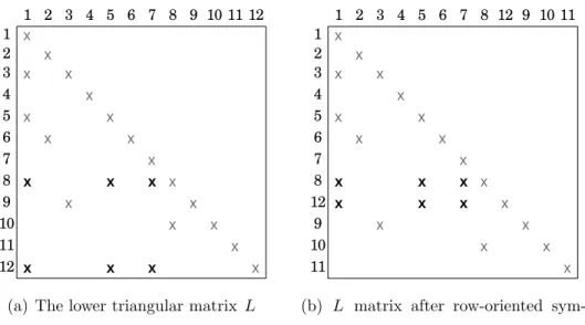
For instance, if we operate a row-oriented forward substitution on the L factor whose nonzero layout is given in Figure 4.1(a), the x1, x5 and x7 entries are used
for solving x8. After completing the calculations for rows 9, 10 and 11, the x1,
x5 and x7 entries are again used for computing x12 because of the nonzeros l12,1,
l12,5 and l12,7. Assuming for this small example that the cache size is not enough
to keep these x entries in the cache for reuse, we operate a symmetric reordering on the L matrix as in Figure 4.1(b) so that rows 8 and 12 become consecutive for exploiting temporal locality.
(a) The lower triangular matrix L (b) L matrix after row-oriented sym-metric reordering
Figure 4.1: Reordering rows of lower triangular factor L for exploiting temporal locality in row-oriented forward substitution
The column-oriented forward substitution algorithm exploits the temporal locality in accesing the x-vector entries which were previously calculated when processing previous columns. Therefore the columns using common xi entries
cache. In order to ensure this, we apply symmetric reordering to the matrix so that the columns having similar nonzero distribution become closer to fit into the cache.
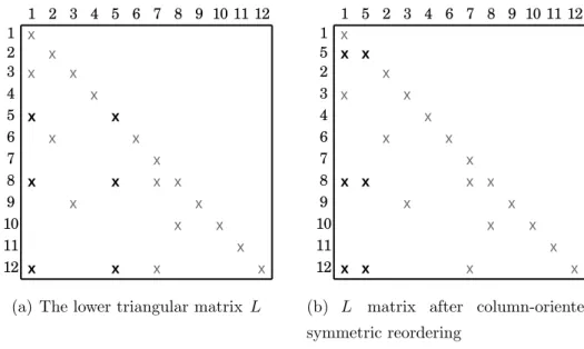
For instance, if we operate a column-oriented forward substitution with the L factor in Figure 4.2(a), the x5, x8 and x12 entries are used for precessing column
1. After completing the calculations for columns 2, 3 and 4, the x5, x8 and x12
entries are again used for processing column 5. Assuming for this small example that the cache size is not enough to keep these x entries in the cache for reuse, we perform a symmetric reordering on the L matrix as illustrated in Figure 4.2(b) so that columns 1 and 5 become consecutive for exploiting temporal locality.
(a) The lower triangular matrix L (b) L matrix after column-oriented symmetric reordering
Figure 4.2: Reordering columns of lower triangular factor L for exploiting tem-poral locality in column-oriented forward substitution
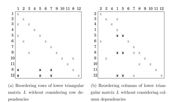
Figure 4.3(a) illustrates the situation if we move row 8 of the L factor in Figure 4.1(a) next to row 12 instead of moving row 12 next to row 8. The nonzero l10,8
appearing in the upper triangular part destroys lower-triangularity and hence the process of forward substitution. The reason for this situation is that we broke the dependency rules by moving row 8 into 11th position despite the fact that
row 10 depends on row 8 because of the nonzero l10,8.
next to column 5 instead of moving column 5 next to column 1 as illustrated in Figure 4.3(b). Here the nonzero l3,1 appears in the upper triangular part because
the dependency rules are broken by moving column 1 into 4th position despite
the fact that column 3 depends on column 1 since l3,1 > 0.
(a) Reordering rows of lower triangular matrix L without considering row de-pendencies
(b) Reordering columns of lower trian-gular matrix L without considering col-umn dependencies
Figure 4.3: Reordering rows/columns without obeying dependency rules would destroy lower-triangularity
Proposition 4.1.1. Obeying dependency rules while doing symmetric reordering is the necessary and sufficient condition for preserving lower triangularity.
Proof. We explained the necessity part in Section 2.4. For proving the sufficiency part, let us assume that lower triangularity is destroyed despite of applying sym-metric reordering by obeying dependency rules. Let the nonzero li,j be placed
on the upper triangular part after reordering to the position (i0, j0). Since li,j is
a nonzero before reordering, we know that i > j and row/column i depends on row/column j . We also know that i0 < j0 since position (i0, j0) stay on the upper triangular part. This means that row/column i is positioned before row /col-umn j by reordering. Since we know that row/col/col-umn i depends on row/col/col-umn j , this fact contradicts with our assumption of obeying dependency rules and completes the proof.
Essentially we do not need to place highly dependent rows consecutively and may even not succeed this hard task every time because of the data dependencies. Theorically, it is enough to place them close enough to exploit temporal locality. Hence we adopt the idea of reordering and partitioning the rows/columns of the triangular factor into parts so that
1. Each part fits into the cache, that is to say the size of the memory required to store the submatrix and the subvectors associated with a part is less than the size of the cache.
2. The data requirements between different parts is minimum, i.e. the number of cache misses induced by the need of accessing data which was previously used in another part is minimum.
3. Part elements obey the data dependency rules, i.e. a part cannot include a row (column) which depends on a row (column) from a subsequent part.
In our model we assume that the cache is fully associative, i.e. any data in the main memory can be stored in any cache location. By this assumption, we do not consider the conflict misses and only take the capacity misses into account.
The first property of this L-factor partitioning means that there will be no cache misses during processing the rows/ columns of the same part if the cache is fully associative. Hence the total number of cache misses is nothing more than the number of cache misses caused by the shared data between different parts. Therefore obeying the second property yields minimizing the total number of cache misses. This property enhances the probability of highly dependent rows / columns belonging to the same part.
4.2
Deficiencies of Directed Graph Partitioning
Model for Reordering Triangular Matrices
In literature, dependence graph representation of lower triangular factor is used to reorder and levelize the rows for parallel implementations [31], [32]. First thing come to mind is that this representation can also be utilized for reordering the rows/ columns of the lower triangular factor by means of graph partitioning tools. We can partition the dependence graph into parts each having weights less than the cache size, and aim to minimize the cutsize which hopefully relates to minimize cache misses.
(a) Partitioning the lower triangular matrix L
(b) Partitioning dependence graph of lower triangular matrix L
Figure 4.4: Partitioning the L factor and corresponding dependence graph
However the cutsize definition of a standard dependence graph representation does not truely encode the cache miss counts. Consider the sample triangular matrix L whose rows are partitioned into 4 parts as shown in the Figure 4.4(a). We assume that each part fits into cache exactly, meaning that adding one more row to a part would end up with no longer fitting into cache. The corresponding dependence graph is constucted and partitioned as in Figure 4.4(b). The initial cut edges are e14, e15, e19, e26, e28 and e47. If we assume that the cost of each
edge is assigned to 1 as a standard graph partitioning setup, then the cutsize will be 6.
Let us consider the traffic of the x1 entry in the cache. First, x1 is calculated
by processing row 1. Then row 3 directly uses x1 value from the cache since
row 1 and 3 belong to the same part which fits into the cache by construction. However row 4 has to fetch x1 from main memory since it is no longer in cache.
Then row 5 can directly get the x1 value from cache since rows 4 and 5 belong
to the same part. Finally row 9 needs x1 value but a cache miss occurs since x1
is ejected from the cache until reaching row 9 from row 5. Therefore there are 2 cache misses induced by data x1 in total, for processing rows 4 and 9. However,
the cutsize arised from vertex v1 of the dependence graph corresponding to the
L factor is 3, namely because of the cut edges e14, e15 and e19. The reason for
this incompability is that the costs of vertices v4 and v5 are counted separately
in the graph partitioning representation for calculating the cutsize although they were needed to be counted once in total.
We see that the graph representation is not adequate for truely encoding the cache-aware forward substitution problem. Yet we propose a novel directed hypergraph partitioning model which is precisely equivalent to lower triangular partitioning problem as described in Section 4.1.
4.3
Directed
Hypergraph
Representation
of
Forward Substitution
Since we see that the graph representation is not adequate for encoding the for-ward substitution to minimize the cache misses, we propose a directed hypergraph model to encode this problem. We adopt a column-net directed hypergraph model for row-oriented forward substitution, and a row-net directed hypergraph model for column-oriented forward substion. The column-net hypergraph model takes its name by the property of the model which assigns the columns of a matrix to the nets of the hypergraph. The row-net hypergraph model is called so beacuse
the rows of the matrix are represented by the nets of hypergraph.
For row-oriented forward substitution, we use a column-net directed hyper-graph model, assigning the rows of the L factor to the vertices of the hyperhyper-graph since we want to permute rows for exploiting temporal locality. The nets are represented by columns of the L factor and net nj consists of the vertices which
correspond to the rows having a nonzero on column j . The directions on hy-peredges are defined as follows: If row i depends on row j , then we say that the net n including vi and vj involve a direction from vj to vi. For the ease of
presentation, we put an arrow going from vj to net n and an arrow going from
net n to vi. Now let us show that the directions of these arrows on a net does
not conflict.
Consider net nj, corresponding to column j . For each nonzero li,j on
col-umn j , row i depends on row j , hence net nj involves a direction from vj to vi.
Therefore net nj involves directions from vertex vj to all other vertices belonging
to the net nj. Then the direction representation is straightforward: There is an
arrow going from vj to net nj and for each other vertex vi in net nj, there is
an arrow from nj to vi. Since such vj vertex is unique to the net nj, we say
that vj is the unique source node of net nj, and all the other vertices belonging
to net nj are called the sink nodes of net nj. We denote the source node of a
net nj as src(nj) for this column-net directed hypergraph model.
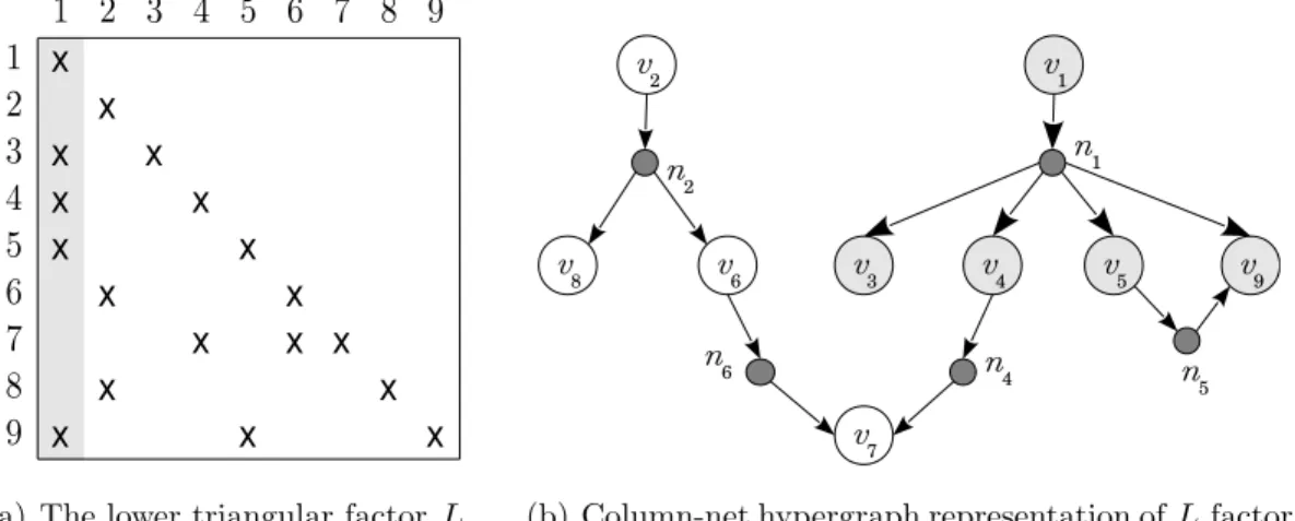
Figure 4.5(b) illustrates the column-net directed hypergraph representation of the L factor given in Figure 4.5(a). The net n1 and corresponding column 1
of the L factor are highlighted. Both rows 3, 4, 5 and 9 depend on row 1 because of the nonzeros l3,1, l4,1, l5,1 and l9,1. Hence net n1 has vertex v1 as a source
(a) The lower triangular factor L (b) Column-net hypergraph representation of L factor
Figure 4.5: Column-net directed hypergraph representation of forward substitu-tion
A similar representation is adopted for column-oriented forward substitution, namely the row-net directed hypergraph model, in which the vertices of the hy-pergraph represent the columns of the L factor since we want to permute columns for exploiting temporal locality. The nets represent the rows of L factor and net nj consists of the vertices which correspond to the columns having a nonzero on
row j . The directions on hyperedges are defined the same as in the column-net model. However in this case we have multiple source nodes and a unique sink node for each net.
Consider net ni, corresponding to row i. For each nonzero li,j lying on row i,
column i depends on column j , hence net ni involves a direction from vj to
vi. Therefore net ni involves directions to vertex vi from all other vertices in
P ins(ni). Hence the direction representation is straightforward: There is an
arrow going from net ni to node vi and there is an arrow from vj to ni for each
vj ∈ P ins(ni) where i 6= j . Vertex vi is called the unique sink node of net ni,
and all the other vertices belonging to net ni are called the source nodes of net
nj in the case of row-net directed hypergraph model.
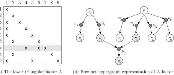
Figure 4.6(b) illustrates the row-net directed hypergraph representation of the L factor given in Figure 4.6(a). The net n7 and corresponding row 7 of the L
on both columns 4 and 6 . Hence net n7 has vertex v7 as a sink node, and the
vertices v4 and v6 as source nodes.
(a) The lower triangular factor L (b) Row-net hypergraph representation of L factor
Figure 4.6: Row-net directed hypergraph representation of forward substitution
4.4
Directed Hypergraph Partitioning (dHP)
In this section we introduce an ordered directed hypergraph partitioning (dHP) model which meets the requirements of the triangular solve partitioning problem. We define an ordered partition on the directed hypergraph to reorder the vertices and hence to permute the corresponding rows/columns of the L factor.
For row-oriented (column-oriented) forward substitution, we define the weight of vertex vi as the number of nonzeros in row (column) i. We assign 1 to the
cost of each net. Our aim is to obtain an ordered partition Π = {V1, . . . , VK} on
the set of vertices so that:
1. The weight of each part Vi is less than the cache size.
2. The cutsize of Π is minimum.
3. If a source of a net n belong to part Vi and a sink node of n belongs to
Let us show that such an ordered partition on the vertices of the directed hypergraph induces a feasible reordering on the rows/ columns of the lower trian-gular factor. Note that these three properties of the aimed directed hypergraph partitioning has one-to-one correspondence with the properties of the desired lower triangular matrix partitioning given in Section 4.1.
Since we assign the number of nonzeros in rows/ columns to the weight of vertices, the weights of the parts in Π correspond to the sizes of the parts in L factor. Therefore making the part weights in Π less than the cache size is equivalent to fitting the parts of L factor into the cache. Hence obeying the first property of the ordered directed hypergraph partitioning induces to fulfill the first property of L factor partitioning defined in Section 4.1.
Minimizing cutsize of Π is equivalent to minimizing the sum of connectivities of cut nets. The connectivity of a net corresponds to the number of parts that the nonzeros of the corresponding row/column belongs to. It is actually the number of cache misses induced by the data requirements of a row / column between different parts if we assume the cache is fully associative. Hence minimizing cutsize of Π corresponds to minimize the number of cache misses arised between different parts, that is to obey the second property of L factor partitioning.
The 3rd property means that the parts should be aligned in the increasing order of their indices by obeying the dependency rules: A sink node of a net must come after a source node, and so do the parts where they belong. Let us denote the part where vertex vi belongs to as part(vi), and the index (order) of a part
P as idx(P). If a net has a source node vs and a sink node vt, then part(vs)
should come before part(vt), meaning that idx(part(vs)) < idx(part(vt)).By this
setup we ensure that there exist no net which involves a direction from a vertex in Vj to a vertex in Vi whenever i < j . Thus this property is directly related to
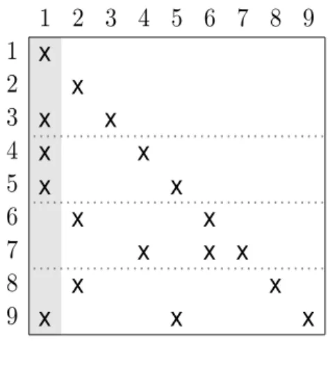
(a) Rowwise partitioning the lower tri-angular matrix L
(b) Partitioning the column-net di-rected hypergraph corresponding to lower triangular matrix L
Figure 4.7: Rowwise partitioning the L factor and the corresponding column-net directed hypergraph
Figure 4.7(b) illustrates the column-net directed hypergraph partitioning cor-responding to the initial rowwise partitioning of the L factor given in Fig-ure 4.7(a). The connectivity set of net n1 is {V1, V2, V3} and the connectivity
of n1 is λ1 = 3. Therefore, net n1 contributes λ1 − 1 = 2 to the cutsize, which
is equal to the number of cache misses induced by entry x1. This equivalence
confirms the applicability and validity of the directed hypergraph partitioning model for the triangular solve reordering problem defined in Section 4.1.
We refer the column-net directed hypergraph partitioning model proposed for exploiting temporal locality in row-oriented forward substitution as row-wise dHP since we define a partition on the rows of the corresponding triangular ma-trix. Similarly we refer the row-net directed hypergraph partitioning model pro-posed for exploiting temporal locality in column-oriented forward substitution as column-wise dHP since we define a partition on the columns of the corresponding triangular matrix.
4.4.1
Recursive Bipartitioning
We solved this K -way partitioning problem by doing recursive bipartitioning until the weight of each part become less than the cachesize. After each bipartitioning step, we apply a variant of FM algorithm which we develop for ordered directed hypergraph partitioning.
Since we are applying recursive bipartitioning, we only consider two parts at each step which we refer to as left and right parts, and denoted as VL and
VR, respectively. We denote the number of pins that net ni has in left part as
Lef t(ni) and the number of pins that ni has in right part as Right(ni).
We assume that the initial partitioning of the vertices obeys the dependency rules, i.e. the arrows between two parts always have directions coming from left part and going to the right part. We preserve this rule by applying a modified FM algorithm that only allows the moves which respect these direction constraints. Note that the initial vertex order corresponding to the original row/ column order is feasible since a net can include a direction from vertex vi to vj only if i < j .
Hence sorting the vertices with increasing order of indices and dividing from any point to two parts yields a partition obeying the dependency rules.
We can handle this initial partition trivially by just splitting the vertex se-quence from the middle, meaning that the weights of each part is approximately equal. Instead, for a better initial bipartitioning, we search the γ neighbourhood of the middle point and split the sequence from the point which yields a minimum initial cutsize. In other words, we start with the first vertex, put it to the left part, and continue this procedure on vertices one by one until the weight of the left part is greater than (50 − γ)% of the total vertex weight. After this point we continue this procedure also by calculating the current initial cutsize and stop when the weight of the left part reaches (50 + γ)% of the total vertex weights. Among the interval that we calculate the initial cutsizes, we determine the vertex index which corresponds to a bipartition with lowest initial cutsize. Then we up-date the part informations of vertices and weight informations of parts according to the bipartitioning which splits the hypergraph from that point.
4.4.1.1 Cut-net Splitting
After completing the initial bipartitioning and our directed FM procedure, we construct two new hypergraphs corresponding to the right and left parts of the bipartition. We proceed these recursive bipartitioning steps onto these two hyper-graphs that we obtain. At this new hypergraph construction step, we duplicate the nets which have nodes in both parts, i.e. the cut nets. This procedure is called cut-net splitting and exploited for capturing the partitioning cutsizes accurately. After each bipartition, we construct two sub-hypergraphs HL and HR
cor-responding to the left and right parts of the bipartitioning respectively. The vertex set of HL (HR) is equivalent to the vertex set of VL (VR). The
inter-nal nets of left (right) part are added to the net set of HL (HR). We split
each cut net ni to two nets nLi and nRi where P ins(nLi ) = P ins(ni) ∩ VL and
P ins(nR
i ) = P ins(ni) ∩ VR.
Note that some nets may not possess a source node or any sink node after this splitting process. For instance assume that the source node v1 of net n1 remains
in left part while the sink nodes v2 and v3 stay in right part after completing
the bipartitioning and the directed FM procedure. Then in the left hypergraph HL we have net nL1 having the source node v1 as its only pin, while in the right
hypergraph HR we have net nR1 having the sink nodes v2 and v3. In this sample
we observe that the net nL1 has no sink nodes in the hypergraph HL and the
net nR1 has no source node in the hypergraph HR. We handle such cases in our
modified FM algorithm.
If we consider the dependencies of the row-net directed hypergraph model oppositely and reverse the directions of the arrows, we obtain nets having a sin-gle source and multiple pins just like our column-net directed hypergraph model. Hence we can apply our partitioning methods proposed for the column-net di-rected hypergraph model to the row-net didi-rected hypergraph model with only a few alterations. For this reason, we assume that the operations are held on the column-net directed hypergraph model for the following algorithms without loss of generality.
4.4.2
Directed Fiduccia-Mattheyses (dFM) Algorithm
For reordering the vertices in order to reduce the cutsize, we developed a vari-ant of FM algorithm which works for directed hypergraph model by taking the dependency rules into account. We refer this modified FM algorithm as directed FM, namely dFM algorithm.As in the usual FM algorithm, we calculate the initial gains of each vertex at the beginning of each bisection for chosing the vertex whose move to other part reduce the cutsize most. For deciding to move the vertex with highest gain (namely the base vertex ), usual FM algorithm only checks the balance constaint given in equation 2.10. However for directed hypergraph model we have two additional feasibility constraints:
1. If the base vertex is the source of net n, and if there exist sink nodes of n in the left part, then the base vertex cannot be moved from left to right part.
2. If the base vertex is a sink node of a net which has the source node in the right part, then the base vertex cannot be moved from right to left part.
If the chosen base vertex yields an unfeasible move, we discard moving this vertex and consider the vertex with the next highest gain value. In order to determine the vertex with highest gain, we use a max-heap assigning the gains of vertices as keys.
The pseudocode of the method IsF easible which checks the feasibility of moving vertex v to other part is shown in Algorithm 3. This procedure returns 1 if moving the corresponding vertex to other part is feasible in terms of dependency rules and 0 otherwise. We consider each net that a given vertex belongs and check if the dependency rules associated with that net are violated in the case of moving the given vertex. We discussed how a net may not have a source vertex in the previous section. The nets which have no source node anymore cannot force the feasibilty constraint and hence are skipped while searching the nets including the given vertex. There are two cases forcing the dependency rules:
1. If the given vertex belongs to the left part and it is the source node of a net that has other vertices in the left part, or
2. If the given vertex belongs to right part and it is a sink node of a net that has its source node in the right part
then we set moving the given vertex to other part as unfeasible and the procedure IsF easible returns 0, otherwise it returns 1.
Algorithm 3 Checking The Feasibility Constraints
1: procedure IsFeasible(v ) 2: for each n ∈ N ets(v) do
3: if n has a source node then
4: s ← src(n)
5: if v = s then
6: if P art(v) = Lef t and Lef t(n) > 1 then
7: return 0
8: else
9: if P art(v) = Right and P art(s) = Right then
10: return 0
11: return 1
Before each move, we extract the vertex with highest gain from the heap and check its feasibility of moving regarding to the dependency constraints and the balance constraint. If moving this vertex is infeasible because of the balance con-straint, we lock this vertex and do not bring it back to the heap. This attitude is applicable and does not restrict the solution space much bacause we observed that the proportion of unfeasible moves due to the balance constraint is highly low compared to the unfeasible moves due to the dependency violation. Morever, the feasibility conditions regarding the dependency constraints frequently change while the vertices moving and altering the node positions of nets. Hence we need a method to reinsert the previously extracted vertices into the heap if they previ-ously extracted from the heap beacuse of the infeasibility regarding dependency constraints but become feasible after a certain move. For this purpose, we check the vertices whose feasibility condition might change from infeasible to feasible and update the max-heap after each move.
We do not update the heap for the vertices turning from feasible to infeasible after each move because we check the feasibility of the base vertex before each move and if it is infeasible we pass to the next element in the heap. Since we handle the detection of vertices which are infeasible to move before moving the base vertex, we do not need to update the heap for evicting the infeasible ones. Hence we do not force the heap to consist of only feasible vertices, but we guarantee that all the feasible vertices belong to the heap in each move.
Algorithm 4 Updating Max-Heap After Moving Base Vertex
1: procedure UpdateHeap(base) 2: for each n ∈ N ets(base) do
3: if n has a source node then
4: s ← src(n)
5: if base = s then
6: if P art(base) = Lef t then
7: for each v ∈ P ins(n) do
8: if v is unlocked and v is not in heap then
9: if IsFeasible (v ) then
10: insert v to heap
11: else if P art(s) = Lef t and Lef t(n) = 1 then
12: if s is unlocked and s is not in heap then
13: if IsFeasible (s) then
14: insert s to heap
Algorithm 4 shows how the max-heap is updated after a move in our dFM algorithm. After each move we consider the vertices whose feasibility condition might change. In general it is enough to check the vertices which share at least one net with the moved (base) vertex. We further restrict our search of the candidate vertices which are possible to turn into feasible condition from infeasible condition. There are two cases that moving a vertex may turn from infeasible to feasible after the move of the base vertex:
1. If base vertex is the source node of net n, and it moved from right part to left part, then the other vertices in P ins(n) which were previosly infeasible might become feasible to move.
part and does not have any other nodes in that part, then the source node of n become feasible to move with respect to the net n.
We continue moving the vertices with highest gain if they are feasible until the heap is empty or no feasible move remains. Then we find the point when the cutsize is minimum and construct the left and right sub-hypregraphs corre-sponding to the vertex distribution at that point. This set of procedures is called a pass of FM algorithm and we apply these passes until the total cutsize gains drop below zero.
4.4.3
Clustering in dHP
We also include a clustering method in our dFM algorithm to ensure placing the highly-dependent rows/columns successively. We construct supernodes for the initial hypergraph and we make the uncoursening after completing all biparti-tioning steps and obtaining the final permutation vector.
Basically we determine the vertices having almost the same set of nets with at most one exception. We connect two vertices vi and vj if the sets N ets(vi)
and N ets(vj) are same except the nets ni and nj for the initial hypergraph, i.e.
if N ets(vi) ∪ {ni, nj} = N ets(vj) ∪ {ni, nj}.
Because of the dependency constraints, we cannot merge each pair of vertices satisfying the above condition. For instance, assume that vertices vi and vj
(i < j) have almost the same set of nets but there exists another vertex vk with
i < k < j such that vk depends on vertex vi and vj depends on vk. Then vi and
vj can belong to the same supernode only if vk is in that supernode too, beacuse
otherwise we encounter with a case that the supernode containing vi and vj both
depends on and is depended by the vertex vk. In order to avoid such cases that
force the dependency constraints, we only allow consecutive vertices to form a supernode.
For each vertex, we consider its adjacent vertex having the next index for checking our clustering criteria. If they satisfy the condition to be connected, then
we embed them in a supernode. We continue this way and add more subsequent vertices to the same supernode until the next vertex does not satisfy the condition to be clustered with the current vertex.
A coarsened hypergraph is constructed such that disjoint subsets of vertices of the original hypergraph which are coalesced into supernodes form a single vertex of this new hypergraph. The weight of a vertex in the coarsened hyper-graph is determined as the sum of the weights of the vertices that constitute the respective supernode in the original hypergraph. To put it more formally, let the vertices vi, vi+1, . . . vj of the original hypergraph H form a supernode which
corresponds to the vertex vi−j0 in the coarsened hypergraph H0. Then we set w(vi−j0 ) = Pj
k=iw(vk). Similarly the net set of vertex v
0
i−j in H
0
is equalized to be the union of the net sets of the constituent vertices vi, vi+1, . . . vj of H , i.e.
N ets(v0i−j) =Sj
k=iN ets(vk).
For the uncoarsening, we project the final partition found on H0 back to a partition on the original hypergraph H . We assign each vertex in H forming a supernode to the part of the corresponding vertex in H0.
In row-net (column-net) directed hypergraph model context, the vertices vi
and vj with almost the same set of nets corresponds to the columns (rows) i
and j having nonzeros in the same rows except the ith and jth rows. In other words, columns (rows) i and i + 1 are coalesced when lk,i 6= 0 holds if and
only if lk,i+1 6= 0 for each k > i + 1, whether li,i+1 is nonzero or not. Hence in
row-net (column-net) directed hypergraph model, clustering stands for combining columns (rows) with similar sparsity patterns.