MONETARY POLICY WITH A FISCAL CONSTRAINT
The Institute of Economics and Social Sciences of
Bilkent University
by
SAİT SİNAN ÖZCAN
In Partial Fulfillment of the Requirements for the Degree of MASTER OF ARTS IN ECONOMICS
in
THE DEPARTMENT OF ECONOMICS BILKENT UNIVERSITY
ANKARA September 2004
MONETARY POLICY WITH A FISCAL CONSTRAINT
A Master’s Thesis
by
SAİT SİNAN ÖZCAN
Department of Economics Bilkent University
Ankara September 2004
I certify that I have read this thesis and have found that it is fully adequate, in scope and in quality, as a thesis for the degree of Master of Arts in Economics.
……… Assistant Prof. Dr. Ümit Özlale Supervisor
I certify that I have read this thesis and have found that it is fully adequate, in scope and in quality, as a thesis for the degree of Master of Arts in Economics.
……… Assoc. Prof. Dr. Hakan Berument Examining Committee Member
I certify that I have read this thesis and have found that it is fully adequate, in scope and in quality, as a thesis for the degree of Master of Arts in Economics.
……… Assoc. Prof. Dr. Levent Özbek Examining Committee Member
Approvel of the Institute Of Economics and Social Sciences
……… Prof. Dr. Erdal Erel
ABSTRACT
MONETARY POLICY WITH A FISCAL CONSTRAINT Özcan, Sait Sinan
M.A., Department of Economics Supervisor: Asst. Prof. Dr. Ümit Özlale
September 2004
The theme of fiscal dominance on monetary policy is an old issue. Basically, in an environment of high debt and high risk premium, inflation targeting does not work well. Higher interest rates lead to higher debt, a higher risk premium, a depreciation, and so, to a higher inflation. In this study, we analyze the influence of fiscal constraints on pursuing monetary policy from the perspective of the risk premium. We use the monthly data of the last three years of the Turkish economy. We obtain the feedback rules for the interest rates by minimizing the loss functions, which include inflation, output gap, and interest rate smoothing as the goal variables. According to the rule obtained under weak fiscal conditions, we observe the negative response of interest rate to inflation, which is the opposite of the rule obtained in absence of high risk premium and debt burden.
ÖZET
MALİ KISITLAR ALTINDA PARA POLİTİKASI Özcan, Sait Sinan
Master, Ekonomi Bölümü
Tez Yöneticisi: Yrd. Doç. Dr. Ümit Özlale
Eylül 2004
Mali durumun para politikalarına olan baskın konumu bilinen bir konudur. Kısaca, yüksek borç yükünün ve risk priminin olduğu bir ekonomide enflasyon hedeflemesi amacına ulaşamamaktadır. Böyle bir ortamda, faiz oranlarının artırılması, sırasıyla borç yükünü, risk primini, devalüasyonu ve sonunda da enflasyonu körüklemektedir. Bu çalışmada, mali kısıtların para politikasına olan etkisi risk primi perspektifinden incelenmektedir. Bunun için Türkiye’nin son üç yıldaki aylık ekonomik verileri kullanılmıştır. Enflasyon, cari açık ve faiz oranları farkından oluşan kayıp fonksiyonlarının minimize edilmesiyle, durum değişkenlerine bağlı optimal faiz oranları elde edilmiştir. Zayıf mali koşullar göz önüne alındığında, optimal faiz oranının enflasyonla ters orantılı olduğu gözlemlenirken, mali kısıtlar göz ardı edildiğinde elde edilen faiz kuralında bu durumun tam ters olduğu görülmüştür.
TABLE OF CONTENTS
ABSTRACT ... iii
ÖZET ... iv
TABLE OF CONTENTS ... v
CHAPTER I: INTRODUCTION ... 1
CHAPTER II: EMERGING MARKET CASES ... 5
II.1. Brazil: A Case Study ... 5
II.2. An Overview of the Turkish Economy ... 9
II.3. Debt Structure of Turkey ... 11
CHAPTER III: METHODOLOGY ... 13
III.1. How is the Loss Function for the Monetary Policy Formed? ... 13
III.2. Monetary Policy Rule: Inflation Targeting ... 14
III.3. Solving the Optimal Linear Regulator Problem (OLRP) ... 20
III.4. The Stochastic Case ... 23
CHAPTER IV: ESTIMATION ... 27
IV.1. The Model ... 27
IV.2. The Optimizers ... 29
IV.3. Estimation Results ... 31
IV.4. Interpretation of the Estimation Results for the Inflation and Output Gap equations .../... 33
CHAPTER V: OPTIMAL RULES UNDER DIFFERENT REGIMES ... 35
V.1. Flexible Inflation Targeting ... 35
V.2. Strict Inflation Targeting ... 37
V.3. Output Targeting .../... 39
V.4. Comparison of Interest Rates ... 41
CHAPTER VI: CONCLUSION ... 42
SELECT BIBLIOGRAPHY ... 44
CHAPTER I
INTRODUCTION
For emerging market economies several financial variables, such as the exchange rate, fluctuate in parallel with the risk premium. One reason is the capital flows: an increase in the risk premium leads to a sudden drop of capital flows and to a depreciation, needed to generate the trade surplus required to offset the decrease in capital flows. On the other hand, fluctuations in the exchange rate induce corresponding fluctuations in the ratio of public debt to GDP. This happens mainly because of the high proportion of dollar denominated debt in the emerging markets.
Domestic interest rates are also affected by fluctuations in the risk premium. In the case of policy rates for the short-run, the mechanism is mostly via the exchange rates: risk premium generates exchange rate fluctuations, which in turn move inflation expectations, and the central bank decides on the policy interest rate according to this newly formed expectations.
In the long run, domestic rates are affected by the risk premium in two ways: indirectly, through the policy interest rate, as mentioned above, because fluctuations in the policy rate move the term structure; and directly because the price of financial instruments of longer maturities reflect interest rate risk, term premium and default risk. Therefore, as a result, the cost of servicing the public debt fluctuates very closely with the risk premium, both in the short and the long run.
Alternatively, Calvo (2002) observed that risk premium is rather correlated with international factors, especially with worldwide measures of investors’ desire for risk, such as the spread between US corporate bonds and US Treasuries. Indeed, Calvo suggests that once one accounts for the US corporate spread, domestic factors appear to be irrelevant while explaining the risk premium. Therefore, his views about the determination of risk premium is different than the ones which stress the importance of exchange rate and public debt in analyzing the risk premium.
In attempt to combine these two distinct views about risk premium, Favero and Giavazzi (2003) presents an evidence for Calvo’s observation, conforming that the Brazilian risk premium is correlated with the US corporate spread, but with some contribution: This correlation is not constant over time, but depends on the state of domestic macroeconomic fundamentals, especially fiscal fundamentals. This inference has important implications especially while designing monetary policy in emerging markets. There may be two different monetary policy regimes depending on the state of fiscal policy. In the good one, the risk premium is low and monetary policy works
in the usual way. However, when fiscal fundamentals are weak, the risk premium is high and economy may shift to a bad equilibrium due to the perverse effects of the monetary policy.
The following scenario happens to be in action in case of implication of monetary policy in a bad equilibrium: with a public debt of short maturity, an increase in the policy interest rate raises the cost of debt service. When the primary budget deficit is fixed, the rise of the debt level triggers the risk premium. This increase in the risk adds to the initial increase in debt, especially if it is accompanied by a depreciation of the exchange rate, which raises the dollar-denominated bonds in terms of domestic GDP. The depreciation affects inflation expectations as well and, eventually, inflation itself. This induces central bank to increase the policy interest rate further, which further triggers the cost of debt service, and so on.
In the light of the above mentioned views, the purpose of this study is to analyze the effects of fiscal constraints on pursuing monetary policy from the perspective of the risk premium. We choose Turkish economy as our case study because of the reasons explained below. First, we minimize loss functions by modeling the economy only with standard inflation and output specifications. In the second case, in order to make a comparison, equations representing the fiscal constraints such as risk premium and ratio of debt over GDP are added to the model. According to the feedback rules obtained from these two different cases we analyze the implications of fiscal dominance on monetary policy. As a result we find that under weak fiscal conditions, the conditional monetary policy methods do not produce expected consequences. Indeed they have perverse effects under high risk premium and debt burden.
CHAPTER II
EMERGING MARKET CASES
In the following sections, we give two case studies. We simply present the Brazilian and Turkish economies as the emerging market cases.
II.1. Brazil: A Case Study
Favero and Giavazzi (2003) estimate a simple model of the Brazilian economy which focuses on a few variables such as the Embi spread, which is a proxy for risk premium, the exchange rate, domestic interest rates, inflation, the survey-based measure of inflation expectations and the dynamics of the public debt. Using this model, they estimate the threshold beyond which the economy might fall into a bad equilibrium: they find that this corresponds to a level of the ratio of the net public debt to GDP. They also analyze the dynamics of the main variables in the bad equilibrium.
Favero and Giavazzi find that in Brazil, inflation expectations are very sticky. Therefore one of the main channels of the interaction between debt and inflation in the fiscal theory is hampered. In absence of fiscal stabilization, an increase in the interest rates triggers inflation through the channel of risk premium, which is the effect of credit risk and term premium responding to a monetary tightening and finally determining the dynamics of the public debt.
Calvo (2002) stresses on the importance of the worldwide measures of the investors’ appetite for risk, such as the spread between US corporate bonds and US Treasuries, in explaining the Brazilian component of the Embi spread. Favero and Giavazzi (2003) observes in Brazil that there is a steady increase in the debt-GDP ratio, partly because the primary surplus, though rising, has never been sufficient to stabilize the debt, in part because, over time, the government has recognized the hidden liabilities especially in the balance sheets of state-owned banks. Therefore the debt level seems to be a factor influencing the response of the Brazilian risk premium to international factors.
Favero and Giavazzi (2003) state that an unsustainable fiscal policy may hinder the effectiveness of monetary policy, to the point that an increase can have a perverse effect on inflation. It is shown that term premium and credit risk reinforce the possibility that a vicious circle might arise, making the fiscal conditions on monetary policy more effective. The experience of Brazil shows how critical the behavior of fiscal policy is. During 2002, Brazil had probably fallen into a bad equilibrium, where
fiscal policy was preventing the effectiveness of monetary policy. However, a small change in the fiscal rule, such as that announced by the new administration in January 2003, has been enough to bring the economy back to normal conditions, and rapidly stabilize the spread, the exchange rate, and through these two variables, inflation expectations, inflation and the dynamics of the public debt.
Blanchard (2003) also studies a similar subject and analyzes the fiscal dominance on inflation targeting. In 2002, the increasing probability that Lula would be elected led to a serious macroeconomic crisis in Brazil. The rate of interest on Brazilian government dollar denominated debt increased sharply, revealing an increase in the market’s assessment of the risk of default. The real exchange rate depreciated sharply against dollar, leading to an increase in inflation. The central bank committed to inflation targeting, and sharply increased the interest rate. The combination of dollar debt and depreciation on the one hand, and sharply increased interest rates on the other, led to government debt dynamics which seemed increasingly difficult to control, further increasing the risk premium. This crisis has subsided as follows: The commitment to a high target for the primary surplus, together with the announcement of a reform of the retirement system, have steadily improved the fiscal outlook over the short and medium run, leading to a decrease in default risk, an appreciation of the real exchange rate, and a decrease in inflation. According to Blanchard (2003), there are a number of lessons to be learned. The one, which has to do with the monetary policy is that, in an environment of high debt, inflation targeting may not work well,
risk of default, a depreciation, and so, to a higher inflation. Bad fiscal conditions may dominate the conventional methods. The evidence shows that in 2002 and 2003 Brazil was in such a condition of this kind, so that, the way to fight inflation is through fiscal policy, not through monetary policy. Fortunately, this appears to be exactly what is happening in Brazil today.
Blanchard discusses the case of taking the influence of interest rate on probability of default on government debt into account. He points out two channels through which the interest rate leads to a decrease in inflation. First, the higher interest rate decreases demand, output, and in turn inflation. Second, the higher interest rate leads to an exchange rate appreciation, which decreases inflation, both directly and indirectly through the induced decrease in demand and output. Blanchard states that in case of bad fiscal conditions such as high overall debt, and risk aversion, an increase in the interest rate leads to a depreciation, rather than an appreciation. Basically, if in response to inflation, the central bank increases the interest rate and that increase leads to a depreciation, this will increase inflation. The more the central bank increases the interest rate, the more it increases the probability of default on government debt, and the more currency depreciates, the more inflation increases.
II.2. An Overview of the Turkish Economy
In order to examine the effects of weak fiscal conditions on the monetary dynamics, the economy, of which we would use the indicators, should have been suffering from inflation, with high interest rates, bad debt structure and high risk premium. For almost 15 years, the Turkish economy has an unsustainable level of real interest rates along with high level of debt-gdp ratio, and of course high risk premium. Therefore it is plausable to use the data of the Turkish economy.
Over the last two decades, the structure of the Turkish economy was quite vulnerable, suffering from high and unsustainable interest rates, mainly due to the pressure of the gradually increasing domestic borrowing of the fiscal sector. This high level of interest rates have almost always induced high risk premium. Under these circumstances it must be mentioned also that the fragility of the banking system made the economy always ready to new crises.
The economic policy was mainly standing on the debt-related financial sources to close the financing gap, because the foreign direct investment was discouraged due to the incomplete financial and institutional infrastructure. In these financial conditions, the domestic banks were borrowing from the international markets in short maturities and extending credit through opening foreign currency positions and accumulating off-balance sheet repo items. This shortened the average maturity of the domestic
borrowing and made the financial stability the primary objective of the monetary authority.
In the second half of the economy, “managed float” was adopted as an extension of the financial stability, aiming to stabilize the real exchange rate. Interest rates were determined by the market, and the public sector was becoming a net foreign debt repayer. This time, the public sector could not generate enough primary surplus and consequently accelerated the domestic borrowing requirement. This happened to be as a pressure on the financial sector, and induced high real interest rates.
Through the end of 1990s, there has been an accumulation of pressure on the economy mainly because of the chronicle budget deficit problem. After the 1998 Russian crisis and the earthquake in 1999, the inflation rate was 68 percent, and fiscal sector borrowing requirement including duty losses reached 29 percent, which was the double of the average of last ten years. The ratio of domestic debt to GDP increased to 42 percent, which was the triple of the average. At this point, a new economic program had been started to decrease inflation and reduce the debt stock to a sustainable level, supported by some structural reforms. At the beginning of the program, interest rates fell very rapidly, due to the already gained credibility. This caused capital inflows, and together with the inflationary dynamics, exchange rate appreciated, leading an expansion of the current account deficits. Structural reforms could not been applied totally, and with the lack of supervision and regulation in the banking sector, economy started to go to a bad equilibrium again. The uncertainties
about the commitment to the economic program influenced the expectations, caused a highly risky environment, and, in the end, the economy was in a severe crisis in February 2001.
A new economic program for strengthening the Turkish economy was adopted, applying a floating exchange rate regime. This new program was intending serious structural changes in the economy. After the adoption of floating exchange rate regime, Central Bank managed to bring the inflation down. This success was crucial for regaining the credibility in the economy. However, in spite of the existence of an independent monetary authority, inflation never fell to a desirable level under the hesitations about the sustainability of the fiscal policy.
This brief analysis of the Turkish economy seems to be evidence on how the eroded fiscal conditions prevent the success of the monetary policy. In order to see the whole picture, we will now look at the debt structure of Turkish economy.
II.3. Debt Structure of Turkey
The debt stock of the Turkish economy mostly consists of short-term debt, mainly indexed to inflation and financial assets. This relationship brings the debt stock management to the center of attention. Basically, the vulnerable debt structure
diminishes the effectiveness of the monetary policy through making the future expectations more sensitive.
Considering the high portion of the short-term debt stock, financing requirement of treasury becomes quite intense. This, of course, requires high debt service and leads to increased fragility of the domestic debt structure. Thus, when the economy faces with any shock, demand for government securities falls and via expectations of monetization of debt, risk of default rises, inducing a pressure on exchange rate and interest rate.
CHAPTER III
METHODOLOGY
As mentioned above, the purpose of this study is to analyze the effects of fiscal constraints on pursuing monetary policy from the perspective of the risk premium. We choose the Turkish economy as our case study and the conclusions are based on the estimations on this data. Therefore, we should introduce the estimation methodology first.
III.1. How is the loss function for the Monetary Policy formed?
We can discuss the effect of fiscal policy on monetary dynamics by using loss functions. We model an inflation-targeting policy regime using loss functions over policy goals. In our loss functions, inflation targeting always involves an attempt to minimize deviations of inflation from the explicit inflation target. In addition, assuming the natural rate hypothesis, our inflation targeting loss functions also
between the specification of the loss function and the specification of an inflation-targeting policy regime, other than inflation variability must enter with a non-negligible weight (see Fischer, Stanley (1996), “Why Are Central Banks Pursuing Long-Run Price Stability?”, King, Mervin A. (1996), “How Should Central Banks Reduce Inflation?- Conceptual Issues”, Taylor, John B. (1996), “How Should Monetary Policy Respond to Shocks While Maintaining Long-Run Price Stability – Conceptual Issues”, Svensson, Lars E.O. (1996) “Commentary: How Should Monetary Policy Respond to Shocks While Maintaining Long-Run Price Stability – Conceptual Issues”). Thus, we interpret inflation targeting as consistent with a conventional quadratic loss function, where in addition to the variability of inflation around the inflation target, there is some weight on the variability of the output gap.
III.2. Monetary Policy Rule: Inflation Targeting
First, it must be said that by an (explicit) instrument rule, we mean that the monetary policy instrument is expressed as an explicit function of available information. Classic examples of instrument rules are the “McCallum rule” (1997, Issues in the Design of Monetary Policy Rules) for the monetary base, or the “Taylor rule” for the federal funds rate. However, by a targeting rule, we mean that the central bank is assigned to minimize a loss function that is increasing in the deviation between a target variable and the target level for this variable. The targeting rule, indeed, implies an implicit instrument rule.
In the literature, the expressions “targeting variable xt”, or “having a target level x* for variable xt” have two meanings. According to the first meaning, the expressions above are used in the sense of “setting a target variable x”. Thus, “having a target” means “using all relevant information to bring the target variable in line with the target”, or more precisely to minimize some loss function over expected future deviations of the target variable from the target level. For instance, the quadratic loss function
min Et
∑
∞ =0 τ δτ (x t+τ - x*)2,where δ, 0<δ<1, is a discount factor and Et denotes the expectations operator conditional on information available in period t.
According to the second meaning, “targeting” and “targets” imply a particular information restriction for the instrument rule, so that the instrument must only depend on the gap between the target variable and the target level. Thus, the instrument rule is restricted to be
A(L)it = B(L)( xt - x*),
A targeting rule for a goal variable is equivalent to having an objective for this variable. Similarly, a targeting rule for an intermediate target variable is equivalent to having a loss function for this intermediate target variable, where the target level sometimes is not constant but depends on current information. The targeting rule can also be expressed as an equation of the target variable, so that the target level for the intermediate target is an explicit function of available information.
Clarida, Gali and Gertler (1999) examine the policy objective of the central bank in a broader fashion. The central bank objective function translates the behavior of the target variables into a welfare measure to guide the policy choice. They assume that this objective function is over the target variables, which are output gap, xt, and inflation, πt.It takes the following form:
max – ½ Et (
∑
∞ =0
i
βi[αx 2t+i + π 2t+i]),
where the parameter α is the relative weight on output deviations. Since xt = yt – zt, the loss function takes potential output zt as the target. It takes the inflation target as zero, but there is no cost in terms of generality since inflation is expressed as a percent deviation from trend.
They emphasize that although there has been a considerable progress in motivating behavioral macroeconomic models from first principles, the same has not been true about rationalizing the objectives of policy. During the past several years, there have been some attempts to obtain a plausible formulation of the policy problem by taking as the welfare criterion the utility of a representative agent within the model.
However, the models that are currently available do not seem to consider the uncertainty that variability of inflation for lifetime financial planning and for business planning. Another limitation is that, while the widely used representative agent approach may be a reasonable way to motivate behavioral relationships, it happens to be highly misleading as a guide to welfare analysis. Briefly, if some groups of people suffer more in recessions than the others in an environment of incomplete insurance and credit markets, then the utility of a hypothetical representative agent might not provide an accurate measure of cyclical fluctuations in welfare.
With certain exceptions, the general approach to this issue is assuming the objective of monetary policy as minimizing the squared deviations of output and inflation from their respective target levels. However, Julio Rotemberg and Michael Woodford (1998) and Woodford (1998) provide a formal justification for this approach. They show that an equation like the one introduced above may be obtained as a quadratic approximation of the utility based welfare function, so that the relative weight α, is a function of the primitive parameters of the model. We will not focus on this issue of
Determining the target rate of inflation is a more immediate question. Another issue is the relative weights assigned to output and inflation losses. The policy makers in the U.S. argue that “price stability” should be the ultimate goal. However, what they propose as price stability is the inflation rate at which inflation is no longer a public concern. In practice, an inflation rate between one and three percent for an industrilized economy seems to meet this definition. A further rearrangement for this criterion is that the official price indices may be overstating the true inflation rate by a percent or two, as argued by the Boskin Commission.
Clarida, Gali and Gertler (1999) discuss the policy problem in the context of policy design under discretion or rules. Generally, the policy problem is to choose a time path for the instrument it to manage time paths of the target variables xt and πt that maximize the objective function presented above. This formulation indeed is in the tradition of the classic Jan Tinbergen (1952) and Henri Theil (1961) “targets” and “instruments” problem. The combination of quadratic loss and linear constraints yields a certainty equivalent decision rule for the path of the instrument. The optimal feedback rule, in general, relates the instrument to the state of the economy.
However, there is an important difference from the classic problem. The target variables depend not only on the current policy, but also on the expectations about future policy. So that, the output gap depends on the future path of the interest rate, and, in turn, inflation depends on the current and expected future behavior of the
output gap. As originally emphasized by Kydland and Prescott (1977), in this kind of environment, credibility of future policy intentions becomes a critical issue. For instance, a credible central bank that can signal the intent to maintain the inflation low in the future, may be able to reduce inflation with a less cost than otherwise.
In this context, the policy makers have the issue of identifying whether it would be desirable to make a credibility-enhancing commitment. This question brings us to the comparison of optimal policy under discretion versus rules. A central bank applying policy under discretion chooses the current interest rate by reoptimizing every period. Any promises in the past do not bind the current policy. On the other hand, under a rule, central bank chooses a plan for the path of the interest rates that it sticks forever.
Clarida, Gali and Gertler emphasize two critical points while comparing the policy under discretion versus rules. The key distinction of the two policies is through the standpoint credibility. It should be answered that whether the current comments constrain the future course of policy in any credible way. In both cases, the optimal outcome is a feedback rule that relates the policy instrument to the current state of the economy. The approaches differ, however, in the implications of the relationship between policy intentions and private sector beliefs. Under discretion, private sector forms its expectations considering how the central bank adjusts policy, knowing that the central bank is free to reoptimize every period. Therefore, considering the rational expectations, the central bank has no incentive to change its plans in an unexpected
consistent”. On the contrary, under a rule, it is basically the binding commitment that makes the policy believable in equilibrium.
Secondly, it is not that much easy to obtain a tightly specified policy rule that could be offered for the use of policy makers with great confidence. However, it is seen to be useful to work through the cases of both discretion and rules in order to develop a set of normative guidelines for policy behavior. As mentioned by Taylor (1993), common sense application of these guidelines may improve the performance of the monetary policy.
III.3. Solving the optimal linear regulator problem (OLRP)
Minimization of the loss function introduced above is indeed solving an optimal linear regulator problem. In this section, we present the solution of the OLRP.
The undiscounted OLRP is to maximize over choice of {ut} t=0∞ the following objective function
∑
∞=0
t
{xt’Rxt + ut’Qut},
subject to xt+1 = Axt + But, x0 given. Here, xt is an (n x 1) vector of state variables, ut is a (k x 1) vector of control variables, R is a negative semidefinite symmetric matrix, Q is a negative definite symmetric matrix, A is an (n x k) matrix. Sargent and Ljungqvist
(2000) guess that the value function is quadratic, V(x) = x’Px, where P is a negative semidefinite symmetric matrix.
The Bellman equation becomes
x’Px = maxu { x’Rx + u’Qu + (Ax + Bu)’P (Ax + Bu) }.
The first order necessary condition for the maximum problem on the right side of the equation is
(Q + B’PB)u = -B’Pax,
which implies the feedback rule for u:
u = -(Q + B’PB)-1B’Pax
or u = -Fx, where
F = (Q + B’PB)-1B’PA.
The above form is called “algebraic matrix Riccati equation” and it expresses the matrix P as an implicit function of the matrices R, Q, A, B. In MATLAB, to obtain the optimum values of the coefficients of the state variables, the loss function (or indeed the return function multiplied by minus one) we use is as follows:
xt’Rxt + ut’Qut + 2ut’Wut.
As stated by Sargent and Ljungqvist under particular conditions, which we will omit here, the matrix Riccati equation has a unique negative semidefinite solution, which is approached in the limit as j → ∞ by the following iterations:
Pj+1 = R + A’PjA – A’PjB(Q + B’PjB)-1B’PjA,
Starting from P0 = 0, where the regarding policy function is
Fj+1 = (Q + B’P jB)-1B’P jA.
The discounted optimal linear regulator problem is to maximize
∑
∞=0
t
subject to xt+1 = Axt + But, x0 given. This problem leads to the following matrix Riccati difference equation modified for discounting:
Pj+1 = R + βA’PjA – β2A’PjB(Q + βB’PjB)-1B’PjA.
The algebraic matrix Riccati equation is modified correspondingly. The value function for the infinite horizon problem is simply V(x0) = x’0Px0, where P is the limiting value of Pj resulting from iterations on equation above, starting from P0 = 0. The optimal policy is ut = -Fxt, where F = β(Q + βB’P jB)-1B’P jA.
We use the Matlab program olrp.m, which can be found in the appendix, to solve the discounted optimal linear regulator problem.
III.4. The Stochastic Case
The stochastic discounted linear optimal regulator problem is to choose a decision for ut to maximize
E
0∑
∞ =0 t βt{xt’Rxt + ut’Qut}, 0 < β < 1,xt+1 = Axt + But + εt+1, t>=0,
where εt+1 is an (nx1) vector of random variables that is independently and identically distributed through time and obeys the normal distribution with mean vector zero and covariance matrix
E εtεt’ = Σ.
The matrices R, Q,A, and B obey the assumption that we have described before.
The value function for this problem is
V(x) = x’Px + d,
where P is the unique negative semidefinite solution of the discounted algebraic matrix Riccati equation corresponding to the Riccati equation described above. As before, it is the limit of iterations starting from P0 = 0. The scalar d is given by
d = β(1- β)-1trP Σ
where “tr” stands for the trace of a matrix. Furthermore, the optimal policy continues to be given by ut = -Fxt, where
F = β(Q + βB’PB)-1B’PA.
A notable feature of this solution is that this feedback rule is identical with the rule for the corresponding nonstochastic optimal linear regulator problem. This outcome is the certainty equivalence principle.
Certainty equivalence principle states that the feedback rule that solves the stochastic optimal linear regulator problem is identical with the rule for the corresponding nonstochastic optimal linear regulator problem.
Proof: Substitute value function given above into the Bellman equation to obtain
V(x) = max{x’Rx + u’Qu + βE[(Ax + Bu + ε)’P (Ax + Bu + ε)] + βd},
where ε is the realization of εt+1 when xt = x and when Eε|x = 0. The preceding equation implies
V(x) = max{x’Rx + u’Qu + βE{x’A’PAx + x’A’PBu + x’A’Pε + u’B’Pax + u’B’Pbu + u’B’Pε + ε’Pax + εPBu + ε’Pε} + βd}.
The first-order condition for u is
(Q + βB’PB)u = -βB’PAx,
which is the feedback rule presented above. Using Eε’Pε = trEε’Pε = trPEεε’ = trPΣ, substituting the feedback rule into the preceding expression for v(x) gives
P = R + βA’PA – β2A’PB(Q + βB’PB)-1B’PA,
and
CHAPTER IV
ESTIMATION
IV.1. The Model
In order to analyze the fiscal constraint on monetary policy, we introduce two equation systems. The first one consists of the following two equations:
πt+1 = α1πt + α2πt-1 + α3πt-2 + α4πt-3 + α5yt + εt+1
yt+1 = β1yt + β2yt-1 – β3(it’ - πt’) + ut+1,
where πt is the monthly inflation; πt’ is the inflation of the last four months, i.e., ¼
∑
= −
3 0
j t j
π ; it is the monthly interest rate announced by Central Bank in percentage points
at an annual rate; it’ is the average interest rate of the last four months, i.e., ¼
∑
= − 3 0 j j t i ;
The first equation relates inflation to a lagged output gap and to lags of inflation. The second equation relates the output gap to its own lags and to the difference between the average funds rate and average inflation over the previous four months. The third term is a simple representation of the monetary transmission mechanism.
We will use the Embi spread as the risk premium. While the empirical evidence consistently shows that one of the main determinants of emerging market spreads are international factors, there are different views about these factors. Kamin and von Kleist (1999) and Eichengreen and Mody (2000) report a negative relationship between the level of long term US interest rates and spreads. Arora and Cerisola (2001) find that the stance and predictability of US monetary policy are also significant in determining capital market conditions in emerging markets. Herrera and Perry (2002) consider both the importance of monetary policy and of the US corporate bond spreads and allow for different long and short run effects, strengthening the evidence on the importance of international factors.
The second equation system consists of the following five equations:
πt+1 = α1πt + α2πt-1 + α3πt-2 + α4πt-3 + α5yt + α6qt + εt+1
yt+1 = β1yt + β2yt-1 – β3(it - πt) + ut+1
prt+1 = ψ1prt + ψ2 t GDP Debt + ξt+1 1 + t GDP Debt = Ф1 t GDP Debt + Ф2it + φt+1
In addition to the first equation system, the second one includes three more equations, providing the effect of fiscal constraint to be examined on the monetary policy. The third equation relates real exchange rate, qt, to its lagged value, to the risk premium, prt, which is taken as Embi spread, and to the interest rate, it. The fourth equation relates risk premium to its lagged value and to the ratio of debt to GDP. The fifth equation relates the ratio of Debt/GDPt to its lagged value and the interest rate.
IV.2. The Optimizers
We interpret inflation targeting as having a loss function for monetary policy, where deviations from an explicit inflation target are given some weight. Our period loss function is
where πt and πt’ are now interpreted as the deviation from a constant given inflation target, and a >= 0 and b >= 0 are the weights on output stabilization and interest rate smoothing, respectively. The variables appearing in the loss function are referred as the goal variables.
Our model has the following state-space representation,
Xt+1 = AXt + Bit + vt+1.
The first equation system has the 9x1 vector Xt of state variables, the 9x9 matrix A, the 9x1 column vector B, and the 9x1 column disturbance vector vt as follows:
Xt = − − − − − − − 3 2 1 1 3 2 1 t t t t t t t t t i i i y y π π π π , A = − + + +
∑
= 8 7 0 5 9 : 7 3 6 2 5 1 4 : 1 3 3 2 1 4 1 5 e e e e e e e e e e e e e j j j y β β β β α α , B = − 0 0 0 0 0 0 0 0 4 3 β , vt = 0 0 0 0 0 0 0 t t u ε .Xt= − − − − − − − 3 2 1 1 3 2 1 t t t t GDP Debt t t t t t t t t i i i pr q y y π π π π , A= + + − + + + + + + + 11 10 0 9 1 9 2 8 1 8 2 7 1 5 12 : 10 3 6 2 5 1 4 : 1 3 3 2 1 7 6 5 5 4 4 3 3 2 2 1 1 e e e e e e e e e e e e e e e e e e e e e e φ ψ ψ γ γ β β β β α α α α α α , B= − 0 0 1 0 0 4 0 0 0 0 2 3 3 φ γ β , vt= 0 0 0 0 0 0 0 t t t t t u ϕ ξ µ ε .
According to the solution of the Matlab code olrp.m, the optimal coefficients of the state variables are obtained for the two equation systems. We minimize the loss functions in case of flexible inflation targeting, strict inflation targeting, and output targeting according to the coefficients of the loss function.
IV.3. Estimation Results
The estimated equations of the first equation system, using the sample period 2001:06 to 2004:06, are shown below:
πt+1 = 275.8 + 1.46πt - 0.49πt-1 – 0.07πt-2 + 0.07πt-3 + 0.4yt + εt+1 R-squared = 0.99, Durbin-Watson = 1.96,
yt+1 = -8.5 + 1.7yt – 0.93yt-1 – 0.0012(it’ - πt’) + ut+1 R-squared = 0.96, Durbin-Watson = 1.33.
The estimated equations of the second equation system are as follows:
πt+1 = 252.8 + 1.49πt - 0.51πt-1 - 0.02πt-2 + 0.02πt-3 + 0.43yt - 1.27qt + εt+1 R-squared = 0.99, Durbin-Watson = 1.99
yt+1 = -8.53 + 1.7yt - 0.93yt-1 – 0.0012(it’ - πt’) + ut+1 R-squared = 0.96, Durbin-Watson = 1.33 qt+1 = -3.11 + 0.51qt + 0.01prt - 0.13it + µt+1 R-squared = 0.28, Durbin-Watson = 1.99 prt+1 = -170 + 0.97prt + 2.3 t GDP Debt + ξt+1 R-squared = 0.85, Durbin-Watson = 1.67 1 + t GDP Debt = 13.3 + 0.9 t GDP Debt - 0.11it + φt+1 R-squared = 0.79, Durbin-Watson = 0.39
IV.4. Interpretation of the estimation results for the inflation and output gap equation:
First System:
When the coefficients of the inflation equation are analyzed, it cannot be rejected that the sum of the coefficients regarding the lagged values of inflation sum to unity. Such a finding implies the existence of an “inflation inertia”. Another important result is the inflationary effect of the output gap: excess demand pressures lead to an increase in the price level, which is consistent with a Phillips curve explanation.
On the other hand, the estimated coefficients for the output gap equation seem reasonable. It can be seen that the monetary policy operates expectedly: an increase in the real interest rate, which is possible by increasing the policy instrument more than the increase in inflation, reduces output gap. Such a finding is consistent with a “Taylor type” monetary policy rule.
Second System:
When the second system of equations is analyzed, the inclusion of the exchange rate in the inflation equation implies the existence of a high degree of exchange rate pass-through. The depreciation of the domestic currency increases both the imported final
degree of exchange rate pass-through is not surprising and shows the existence of “indexation” for most of the emerging markets: when the initial rate of inflation is high, agents in the economy views the changes in the exchange rate as some kind of an “anchor”. When the equation for the exchange rate is observed, some unconventional results are obtained. For example, an increase in the EMBI spread leads to appreciation. This finding is explained only if the investors have increasing incentives to take risks for the observed sample period. On the other hand, the uncovered interest rate parity condition works unexpectedly. Such a finding is also common when the emerging markets are analyzed. Finally, when the risk premium equation is observed, we see that, as expected, an increase in the debt to GDP ratio leads to a more than one-to-one increase in the risk premium.
CHAPTER V
OPTIMAL RULES UNDER DIFFERENT REGIMES
V.1. Flexible inflation targeting
In case of flexible inflation targeting, the loss function according to the regarding coefficients is
Lt = πt’2 + yt2 + 0.5(it – it-1)2.
First, in the case of two equations, in other words when there is no fiscal constraint, the feedback rule is
i = 1.1095πt – 0.5633πt-1 + 0.0056πt-2 + 0.0823πt-3 + 1.8357yt – 2.0376yt-1 + 0.916it-1 – 0.0019it-2 – 0.0009it-3
i = -2.1041πt + 1.0768πt-1 - 0.0015πt-2 - 0.0436πt-3 - 4.4355yt + 3.7745yt-1 + 5.226qt +
0.3256prt + 1.7759
t
GDP Debt
+ 0.4518it-1 + 0.0023it-2 – 0.0012it-3
After the optimization is performed via optimal linear regulator problem with the weights given above, two “interest rate rules” are obtained: one for the economy without any fiscal constraints and the other one with the debt burden.
When the first rule is observed, it can be seen that the interest rate responds less agressively to inflation. However, such a finding can be seen as a sign of accommodative policy since we observe that interest rates also decrease due to an increase in the output gap. However, the sum of the coefficients is around –0.21, which implies that the optimal policy requires a slight response of interest rates to demand pressures. Finally, and not surprisingly, we see that the interest rates follow rather an autoregressive process: the coefficient of the lagged interest rate is close to unity.
The results become much more important when the fiscal fundamentals are added to the system as additional constraints. In this case, the optimal policy changes significantly. The interest rates and the inflation is negatively related, providing support for the arguments of Blanchard (2003) and Favero and Giavazzi (2003). If the interest rates increase due to an increase in the inflation, then it is possible to observe some kind of a “prize puzzle”, where increased interest rates actually lead to an
increase in the risk perceptions of the investors, and result in a depreciation of the domestic currency. Given that there is a high degree of exchange rate pass-through, a depreciation of the currency actually leads to an increase in the price level. The argument of the response of the interest rates to output gap remains largely the same. Besides, we obtain a positive relation between exchange rate and the interest rate: an appreciation of the currency leads to an increase in the interest rate, possibly by an increased demand for the domestic currency. Also, both the coefficients regarding the debt to GDP stock and the risk premium lead to an increase in the interest rates, as expected.
V.2. Strict inflation targeting
The following loss function is minimized in case of strict inflation targeting.
Lt = πt’2 + 0.5yt2 + 0.5(it – it-1)2.
The feedback rule without a fiscal constraint is as follows:
i = 1.1110πt – 0.5642πt-1 + 0.0057πt-2 + 0.0824πt-3 + 1.8852yt – 2.0526yt-1 + 0.916it-1 – 0.0019it-2 – 0.0009it-3
i = -2.1044πt + 1.0769πt-1 - 0.0016πt-2 - 0.0436πt-3 - 4.4617yt + 3.8069yt-1 + 5.227qt +
0.3257prt + 1.7758
t
GDP Debt
+ 0.4519it-1 + 0.0023it-2 – 0.0012it-3
When we perform the optimization of the loss function presented above, we obtain these two feedback rules, where the second one has a fiscal constraint.
Actually, the rule of strict inflation targeting is more or less the same with the one obtained in flexible inflation targeting. Again, the response of inflation is greater in case of having weak fiscal conditions than of ignoring the fiscal constraint. Also the total effect of output gap on interest rate is still negative with a coefficient of -0.17. Finally, as the coefficients of the lagged variables of interest rate remained unchanged, the interest rates still follow an autoregressive process.
Addition of fiscal constraints results in a feedback rule very similar to that of flexible inflation targeting. Interest rates respond inflation negatively and with a greater coefficient. Therefore, in case of high inflation, an increase in interest rates induces high risk premium, and in turn causes depreciation, where in most emerging markets depreciation triggers inflation. In strict inflation targeting, the negative effect of output gap remains almost the same. Also as in flexible inflation targeting, an appreciation leads to higher interest rates most probably due to an increase in the demand of
domestic currency. Finally, not surprisingly, risk premium and debt-to-GDP ratio have positive effects on interest rates.
Consequently, either in “flexible” or ”strict” form, inflation targeting regimes produce similar results when fiscal constraints are accounted for. Such a result implies that, in case of weak fiscal conditions, there is not much importance of the monetary policy.
V.3. Output targeting
In case of output targeting, the greatest coefficient is given to the output gap and the follwing loss function is minimized:
Lt = πt’2 + 2yt2 + (it – it-1)2.
The feedback rule obtained when there is no fiscal constraint is
i = 0.6796πt – 0.3451πt-1 + 0.0034πt-2 + 0.0504πt-3 + 1.0699yt – 1.2005yt-1 + 0.934it-1 – 0.0011it-2 – 0.0005it-3
When we impose the fiscal constraints under output targeting the following rule is obtained:
i = -1.4204πt + 0.7308πt-1 - 0.0013πt-2 - 0.0295πt-3 - 2.9230yt + 2.4942yt-1 + 3.595qt +
0.2572prt + 1.5904
t
GDP Debt
+ 0.4829it-1 + 0.0015it-2 + 0.0008it-3
In output targeting policy regime, when we look at the loss function, the coefficient of output gap is greater than the coefficients of inflation and interest rate smoothing.
According to the first system of equations, it is apparently seen that the response of inflation and output gap became weaker in case of output targeting. Inflation has still a positive effect on interest rate, but less aggressively. The negative total response of output gap to interest rate remains almost the same with a coefficient of –0.13. Also as the coefficient of lagged interest rate is still close to unity, interest rates seem to have an autoregressive process.
The most important consequence of addition of fiscal constraints, as seen in the flexible and strict inflation targeting, is the negative and more aggressive response of inflation to interest rate. This negative relation occurs again through the channel of high risk premium and depreciation causing inflation when the interest rates increase in case of weak fiscal conditions. Output gap responds negatively as in the cases of inflation targeting. Also, appreciation induces an increase in the interest rates due to the increased demand for domestic currency. However, this response of the change of real exchange rate parity stays rather smaller when compared to the cases of flexible
and strict inflation targeting. Finally, as expected, there is positive response of risk premium and debt-to-GDP ratio in case of output targeting too.
V.4. Comparison of Interest Rates
These three targeting policy regimes reflect the differences by coefficients in their feedback rules. When we look at the flexible and strict inflation targeting feedback rules, we see a very small difference. This small difference appears to be the slightly higher absolute effect of output gap on interest rate in the strict inflation targeting than that of the flexible targeting policy regime. However, output targeting policy regime has some clearer distinctions. In the case of giving a higher weight on output gap, the effect of inflation on interest rate apparently decreases. In fact, this decrease appears also in the effects of output gap, real exchange rate, risk premium, and debt-to-GDP ratio.
CHAPTER VI
CONCLUSION
The model and the empirical work yield a clear conclusion that in case of weak fiscal conditions, an increase in the interest rate leads to even a higher inflation than the previous one. This situation totally contradicts with what the traditional methods suggest. In general, an increase in the interest rate leads to a decrease in inflation through two channels. First, the higher interest rate decreases demand, output, and in turn, inflation. Second, the higher interest rate leads to an exchange rate appreciation. The appreciation decreases inflation, both directly, and indirectly through the induced decrease in demand and output. However, there is a perverse effect of increasing the interest rate under a fiscal constraint. This effect calls into question the logic of inflation targeting, where the interest rate responds positively to inflation. If in response to inflation, the monetary authority increases the interest rate, and the interest rate leads to a depreciation, finally this will increase inflation. The more the central bank increases the interest rate, the more it increases the risk premium,and the more the currency depreciates, the more inflation increases.
We used the data of Turkish economy due to the fact that it has a rather high risk premium and debt burden. We compared the interest rate feedback rules obtained with and without a fiscal constraint. We solved the optimal linear regulator problem in order to obtain the feedback rules in both cases. When there is no fiscal constraint we observe the positive relationship between the interest rate and inflation. Also we see the negative response of output gap. Another consequence of the first rule is that the interest rates follow an autoregressive process.
When the fiscal fundementals are added, the optimal policy rule changes significantly. In case of having fiscal constraints, the policy rule supports our claim so that we observe a negative response of interest rate to inflation. When the monetary authority increases interest rate due to an increase in inflation, this will lead to an increase in the risk perceptions of the investors, and result in a depreciation of the domestic currency. Assuming that there is a high degree of exchange rate pass-through, this depreciation leads to inflation. The response of interest rate to output gap is negative on the aggregate again. Finally, both the debt-to-GDP ratio and the risk premium lead to an increase in the interest rates.
SELECT BIBLIOGRAPHY
Arora,V. and M. Cerisola (2001), “How Does U.S. Monetary Policy Influence Sovereign Spreads in Emerging Markets?”, IMF Staff Papers 48(3):474-98.
Blanchard, Olivier (2003), “Fiscal dominance and inflation targeting. Lessons from Brazil.”
Calvo, Guillermo (2002), “Explaining sudden stop, growth collapse and BOP crisis”. 2002 Mundell-Fleming Lecture, IMF Staff Papers.
Clarida, R., J. Gali, M. Gertler (1999), “The Science of Monetary Policy: A New Keynesian Perspective”, NBER Working Paper No. 7147.
Eichengreen B. and A. Mody (2000), “What explains changing spreads on emerging market debt?”, Capital flows and the emerging economies: Theory, evidence, and
controversies, S. Edwards ed., NBER Conference Report series. Chicago and London:
University of Chicago Press, 200;107-34.
Favero, Carlo and Giavazzi, Francesco (2003), “Monetary policy when debt and default risk are high. Lessons from Brazil.”mimeo, Bocconi.
Fischer, Stanley (1996), “Why Are Central Banks Pursuing Long-Run Price Stability?”, Federal Reserves Bank of Kansass City.
Herrera, S. and G. Perry (2002), “Determinants of Latin spreads in the new economy era: the role of U.S. interest rates and other external variables”, mimeo, the World
Bank.
Kamin S.B. and von Kleist (1999), “The evolution and determinants of emerging market credit spreads in the 1990s”, Board of Governors of the Federal Reserve
System, IFDP 653.
King, Mervin A. (1996), “How Should Central Banks Reduce Inflation?-Conceptual Issues”, Federal Reserves Bank of Kansas City.
Kydland Finn E. and Edward C. Prescott (1977), “Rules Rather Than Discretion: The Inconsistency of Optimal Plans”, Journal of Political Economy 85, pp.473-491.
McCallum, Bennett (1997), “Issues in the Design of Monetary Policy Rules”, NBER
Working Paper No. 6016.
Rotemberg, Julio and Woodford, Michael (1998), “Interest Rate Rules in an Estimated Sticky Price Model”, Monetary Policy Rules, edited by John B. Taylor.
Rudebusch, Glenn D. and Lars E.O. Svensson (1998), “Policy Rules For Inflation Targeting”, Working Paper No. 6512.
Sargent, Thomas and Lars Ljungqvist (2000), “Recursive Macroeconomic Theory”, The MIT Press, Cambridge, Massachusetts.
Svensson, Lars E.O. (1996), “Commentary: How Should Monetary Policy Respond to Shocks while Maintaining Long-Run Price Stability-Conceptual Issues”, Federal
Reserves Bank of Kansas City.
Taylor, John B. (1993), “Discretion versus Policy Rules in Practice”,
Carnegie-Rochester Series on Public Policy 39, 195-214.
Taylor, John B. (1996), “How Should Monetary Policy Respond to Shocks while Maintaining Long-Run Price Stability-Conceptual Issues”, Federal Reserves Bank of
Kansas City.
Theil, Henri (1961), “Economic Forecasts and Policy”, 2nd edition, Amsterdam, North Holland.
Tinbergen, Jan (1952), “On the Theory of Economic Policy”, 2nd edition, Amsterdam, North Holland.
APPENDIX
Figure 1: EMBI Spread between June 2001 and June 2004
Figure 2: Percentage of Debt/GDP between June 2001 and June 2004
Figure 3: Monthly inflation between June 2001 and June 2004
EMBI Spread 0 200 400 600 800 1000 1200 1 4 7 10 13 16 19 22 25 28 31 34 37 2001:06 - 2004:06 EMBI Spread Series1 Percentage of Debt/GDP -20,00 40,00 60,00 80,00 100,00 120,00 1 4 7 10 13 16 19 22 25 28 31 34 37 2001:06 - 2004:06 Debt/GDP % Series1 Monthly Inflation -0,01 0 0,01 0,02 0,03 0,04 0,05 0,06 0,07 1 4 7 10 13 16 19 22 25 28 31 34 37 2001:06 - 2004:06 Inflation Rate Series1
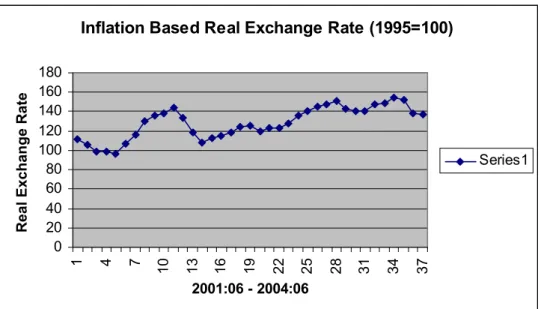
Figure 4: Inflation based real exchange rate between June 2001 and June 2004
MATLAB CODES
Matlab code for flexible inflation targeting without a fiscal constraint beta = 1; A = [1.46 -0.49 -0.07 0.07 0.40 0 0 0 0; 1 0 0 0 0 0 0 0 0; 0 1 0 0 0 0 0 0 0; 0 0 1 0 0 0 0 0 0; 0.0004 0.0004 0.0004 0.0004 1.7 -0.93 -0.0004 -0.0004 -0.0004; 0 0 0 0 1 0 0 0 0; 0 0 0 0 0 0 0 0 0; 0 0 0 0 0 0 1 0 0; 0 0 0 0 0 0 0 1 0] B = [0;0;0;0;-0.0004;0;1;0;0] Q = -1*[1/16 0 0 0 0 0 0 0 0; 1/8 1/16 0 0 0 0 0 0 0; 1/8 1/8 1/16 0 0 0 0 0 0;
Inflation Based Real Exchange Rate (1995=100)
0 20 40 60 80 100 120 140 160 180 1 4 7 10 13 16 19 22 25 28 31 34 37 2001:06 - 2004:06
Real Exchange Rate
0 0 0 0 1 0 0 0 0; 0 0 0 0 0 0 0 0 0; 0 0 0 0 0 0 0.5 0 0; 0 0 0 0 0 0 0 0 0; 0 0 0 0 0 0 0 0 0] R = -0.5 W = [0;0;0;0;0;0;0.5;0;0] %function [f,p] = olrp(beta,A,B,Q,R,W) %function [f,p] = olrp(beta,A,B,Q,R,W)
%%OLRP can have arguments: (beta,A,B,Q,R) if there are no cross products % (i.e. W=0). Set beta=1, if there is no discounting.
%
% OLRP calculates f of the feedback law: %
% u = -fx
%
% that maximizes the function: %
% sum {beta^t [x'Qx + u'Ru +2x'Wu] } %
% subject to
% x[t+1] = Ax[t] + Bu[t] %
% where x is the nx1 vector of states, u is the kx1 vector of controls, % A is nxn, B is nxk, Q is nxn, R is kxk, W is nxk.
%
% discrete matrix Riccati equation. %
m=max(size(A)); [rb,cb]=size(B);
if nargin==5; W=zeros(m,cb); end; if min(abs(eig(R)))>1e-5; A=sqrt(beta)*(A-B*(R\W')); B=sqrt(beta)*B; Q=Q-W*(R\W'); [k,s]=doubleo(A',B',Q,R); f=k'+(R\W'); p=s; else; p0=-.01*eye(m); dd=1; it=1; maxit=1000;
% check tolerance; for greater accuracy set it to 1e-10 while (dd>1e-6 & it<=maxit);
f0= (R+beta*B'*p0*B)\(beta*B'*p0*A+W'); p1=beta*A'*p0*A + Q -(beta*A'*p0*B+W)*f0; f1= (R+beta*B'*p1*B)\(beta*B'*p1*A+W');
dd=max(max(abs(f1-f0))); it=it+1;
p0=p1; end; f=f1;p=p0;
if it>=maxit; disp('WARNING: Iteration limit of 1000 reached in OLRP'); end; end;
Matlab code for flexible inflation targeting with a fiscal constraint beta = 1; A = [1.49 -0.51 -0.02 0.02 0.43 0 -1.27 0 0 0 0 0; 1 0 0 0 0 0 0 0 0 0 0 0; 0 1 0 0 0 0 0 0 0 0 0 0; 0 0 1 0 0 0 0 0 0 0 0 0; 0.0003 0.0003 0.0003 0.0003 1.7 -0.93 0 0 0 -0.0003 -0.0003 -0.0003; 0 0 0 0 1 0 0 0 0 0 0 0; 0 0 0 0 0 0 0.51 0.013 0 0 0 0; 0 0 0 0 0 0 0 0.97 2.3 0 0 0; 0 0 0 0 0 0 0 0 0.9 0 0 0; 0 0 0 0 0 0 0 0 0 0 0 0; 0 0 0 0 0 0 0 0 0 1 0 0; 0 0 0 0 0 0 0 0 0 0 1 0] B = [0;0;0;0;-0.0003;0;-0.013;0;-0.11;1;0;0] Q = -1*[1/16 0 0 0 0 0 0 0 0 0 0 0; 1/8 1/16 0 0 0 0 0 0 0 0 0 0; 1/8 1/8 1/16 0 0 0 0 0 0 0 0 0; 1/8 1/8 1/8 1/16 0 0 0 0 0 0 0 0; 0 0 0 0 1 0 0 0 0 0 0 0; 0 0 0 0 0 0 0 0 0 0 0 0;
0 0 0 0 0 0 0 0 0 0 0 0; 0 0 0 0 0 0 0 0 0 0 0 0; 0 0 0 0 0 0 0 0 0 0.5 0 0; 0 0 0 0 0 0 0 0 0 0 0 0; 0 0 0 0 0 0 0 0 0 0 0 0] R = -0.5 W = [0;0;0;0;0;0;0;0;0;0.5;0;0] %function [f,p] = olrp(beta,A,B,Q,R,W) %function [f,p] = olrp(beta,A,B,Q,R,W)
%%OLRP can have arguments: (beta,A,B,Q,R) if there are no cross products % (i.e. W=0). Set beta=1, if there is no discounting.
%
% OLRP calculates f of the feedback law: %
% u = -fx
%
% that maximizes the function: %
% sum {beta^t [x'Qx + u'Ru +2x'Wu] } %
% subject to
% x[t+1] = Ax[t] + Bu[t] %
% where x is the nx1 vector of states, u is the kx1 vector of controls, % A is nxn, B is nxk, Q is nxn, R is kxk, W is nxk.
%
% Also returned is p, the steady-state solution to the associated % discrete matrix Riccati equation.
%
m=max(size(A)); [rb,cb]=size(B);
if nargin==5; W=zeros(m,cb); end; if min(abs(eig(R)))>1e-5; A=sqrt(beta)*(A-B*(R\W')); B=sqrt(beta)*B; Q=Q-W*(R\W'); [k,s]=doubleo(A',B',Q,R); f=k'+(R\W'); p=s; else; p0=-.01*eye(m); dd=1; it=1; maxit=1000;
f0= (R+beta*B'*p0*B)\(beta*B'*p0*A+W'); p1=beta*A'*p0*A + Q -(beta*A'*p0*B+W)*f0; f1= (R+beta*B'*p1*B)\(beta*B'*p1*A+W'); dd=max(max(abs(f1-f0))); it=it+1; p0=p1; end; f=f1;p=p0;
if it>=maxit; disp('WARNING: Iteration limit of 1000 reached in OLRP'); end; end;