© TÜBİTAK
doi:10.3906/elk-1806-221 h t t p : / / j o u r n a l s . t u b i t a k . g o v . t r / e l e k t r i k /
Research Article
The biobjective multiarmed bandit: learning approximate lexicographic optimal
allocations
Cem TEKİN∗,
Department of Electrical and Electronics Engineering, Faculty of Engineering, Bilkent University, Ankara, Turkey
Received: 29.06.2018 • Accepted/Published Online: 10.12.2018 • Final Version: 22.03.2019
Abstract: We consider a biobjective sequential decision-making problem where an allocation (arm) is called ϵ lexi-cographic optimal if its expected reward in the first objective is at most ϵ smaller than the highest expected reward, and its expected reward in the second objective is at least the expected reward of a lexicographic optimal arm. The goal of the learner is to select arms that are ϵ lexicographic optimal as much as possible without knowing the arm reward distributions beforehand. For this problem, we first show that the learner’s goal is equivalent to minimizing the ϵ lexicographic regret, and then, propose a learning algorithm whose ϵ lexicographic gap-dependent regret is bounded and gap-independent regret is sublinear in the number of rounds with high probability. Then, we apply the proposed model and algorithm for dynamic rate and channel selection in a cognitive radio network with imperfect channel sensing. Our results show that the proposed algorithm is able to learn the approximate lexicographic optimal rate–channel pair that simultaneously minimizes the primary user interference and maximizes the secondary user throughput.
Key words: Multiarmed bandit, biobjective learning, lexicographic optimality, dynamic rate and channel selection, cognitive radio networks
1. Introduction
The multiarmed bandit (MAB) is used to model real-world applications in which the decision maker repeatedly interacts with its unknown environment in order to maximize its long-term reward [1, 2]. The decision maker can be a recommender system recommending items to its users [3], a secondary user performing opportunistic spectrum access in a cognitive radio network [4], or an agent that chooses a routing path between the source and the destination in a network [5].
A plethora of prior works on the MAB focused on designing learning algorithms that optimize the total scalar reward. These include the celebrated upper confidence bound (UCB) policies [1,6] and posterior sampling [2, 7]. On the other hand, in many real-world applications of the MAB, the environment produces vector-valued rewards, where each component of the reward vector corresponds to a different goal. For instance, in a cognitive radio network, the goal of the secondary user (SU) is to maximize its throughput while minimizing the interference to the primary user (PU). In this paper, we introduce the biobjective MAB to tackle this type of sequential decision-making problems. In the biobjective MAB, the learner receives, at each round, random rewards from two objectives. These objectives are lexicographically ordered in the sense that the learner values the first objective more than the second objective.
The learner aims at selecting approximate lexicographic optimal allocations (arms), which yield an ϵ
∗Correspondence: [email protected]
optimal expected reward in the first objective and an expected reward that is at least the expected reward of a lexicographic optimal arm in the second objective. This notion of optimality allows the learner to accumulate a high reward in the second objective by incurring a small loss in the first objective. In order to quantify the loss of the learner due to not knowing the ϵ lexicographic optimal arms beforehand, we introduce the notion of
ϵ lexicographic regret, and propose a learning algorithm whose ϵ lexicographic gap-dependent regret is O(1)
and gap-independent regret is ˜O(√T ) with high probability. Then, we cast the dynamic rate and channel
selection problem in a cognitive radio network with imperfect channel sensing as a biobjective MAB where the first objective is related to PU interference and the second objective is related to SU throughput.
To sum up, in this work, we propose a new MAB called the biobjective MAB, study the notion of approximate lexicographic optimality, propose a learning algorithm and bound its regret, and investigate a multirate multichannel communication application of the biobjective MAB. The algorithm we propose is fundamentally different from the algorithms designed to learn in the MAB with scalar reward and uses confidence intervals, in addition to the UCBs, in order to learn the optimal arms based on lexicographic ordered objectives. This also makes the regret analysis substantially different from the prior work, since bounding the regret requires considering the confidence intervals for both objectives.
2. Related work
In the classical MAB, first studied in [2], at each round, after selecting an arm, the learner receives a random reward that comes from an unknown distribution that depends on the selected arm. An asymptotically optimal adaptive allocation rule with O(log T ) regret is proposed in [1] for the classical MAB with independent arms. Later, finite time O(log T ) regret bounds are derived in [6]. It is also shown in [1] that when the arms are independent, the best possible regret is O(log T ). Numerous interesting extensions of the classical MAB are proposed later on, including the combinatorial MAB [8] and the unimodal MAB [9,10].
For instance, [8] proposes the combinatorial MAB in which the learner selects at each round a super arm that is composed of multiple arms, observes the outcomes of the selected arms, and receives a linear combination of the rewards of the selected arms. The combinatorial bandit is used in [11] to learn the optimal allocations in a multiuser multichannel communication system. Due to obtaining observations from each selected arm, this problem is also called the combinatorial semibandit [12]. Reward functions that are nonlinear in the expected outcomes of arms are considered in [13] and [14].
The variant of the classical MAB we consider in this paper is the multiobjective MAB. Unlike the classical MAB, where the reward is scalar, the reward is vector valued in the multiobjective MAB. This results in various notions of optimality, each of which require a different learning algorithm. For instance, Pareto optimality is considered in [15], [16], and [17]. Essentially, an arm is called Pareto optimal, if switching to any arm that is better in terms of the expected reward in at least one objective will result in a reduction in the expected reward in at least one other objective. It is shown that the Pareto regret, i.e. the loss due to not selecting arms from the Pareto front, is O(log T ) . As an extension, contextual multiobjective MAB with similarity information is considered in [18]. In this work, the authors propose a multiobjective learning algorithm that uses the contextual zooming idea [19], and prove that the Pareto regret is ˜O(T(1+dp)/(2+dp)) where d
p is the Pareto zooming dimension of the similarity space.
Another important notion of optimality in the multiobjective setting is lexicographic optimality [20]. Unlike Pareto optimality in lexicographic optimality, the order of the objectives matter. In this case, the
learner prefers obtaining higher reward in any objective i to obtaining higher reward in any other objective j such that i < j . Lexicographic optimality is first studied in a contextual MAB [21,22], and it is shown that the lexicographic regret is ˜O(T(2+d)/(3+d)) , where d is the dimension of the context set. In addition to the
MAB, the notions of Pareto optimality and lexicographic optimality are also considered in the more general reinforcement learning framework [23,24].
Compared to all the works mentioned above, in this paper, we propose the biobjective MAB with approximate lexicographic optimality as the performance metric for the first time. As opposed to lexicographic optimality, we analyze the learner’s performance when it can tolerate ϵ > 0 suboptimality in the first objective. This way, the learner seeks to identify and select ϵ optimal arms in the first objective, which might result in significant improvement in the reward it obtains in the second objective. We prove two high probability bounds on the ϵ lexicographic regret: O(1) gap-dependent regret bound and ˜O(√T ) gap-independent regret bound.
These bounds are much sharper than the ˜O(T(2+d)/(3+d)) regret bound for the multiobjective contextual MAB, since the existence of contexts makes learning of lexicographic optimal allocations more difficult.
3. Problem formulation
In this section, we explain the system model, and define approximate lexicographic optimality and the regret. Our notation is presented in Table1.
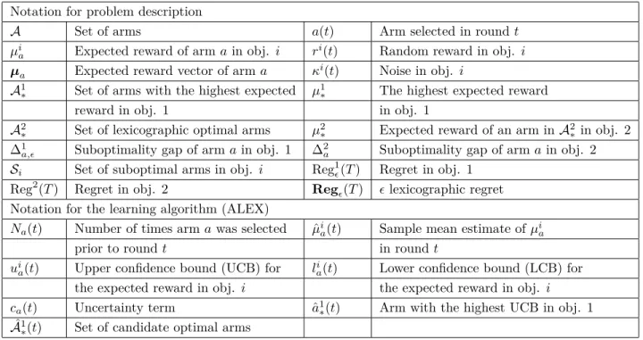
Table 1. Notation
Notation for problem description
A Set of arms a(t) Arm selected in round t
µi
a Expected reward of arm a in obj. i ri(t) Random reward in obj. i µa Expected reward vector of arm a κi(t) Noise in obj. i
A1
∗ Set of arms with the highest expected µ1∗ The highest expected reward
reward in obj. 1 in obj. 1
A2
∗ Set of lexicographic optimal arms µ2∗ Expected reward of an arm in A2∗in obj. 2 ∆1a,ϵ Suboptimality gap of arm a in obj. 1 ∆2a Suboptimality gap of arm a in obj. 2
Si Set of suboptimal arms in obj. i Reg1ϵ(T ) Regret in obj. 1 Reg2
(T ) Regret in obj. 2 Regϵ(T ) ϵ lexicographic regret
Notation for the learning algorithm (ALEX)
Na(t) Number of times arm a was selected µˆia(t) Sample mean estimate of µia
prior to round t in round t
ui
a(t) Upper confidence bound (UCB) for lai(t) Lower confidence bound (LCB) for the expected reward in obj. i the expected reward in obj. i
ca(t) Uncertainty term ˆa1∗(t) Arm with the highest UCB in obj. 1 ˆ
A1
∗(t) Set of candidate optimal arms
3.1. System model
We consider decision epochs (rounds) indexed by t ∈ {1, 2, . . .}. At each round t, the learner first selects
denoted by ri(t) , which is equal to µi a(t)+ κ
i(t) , where µi
a denotes the expected reward of arm a in objective
i and κi(t) denotes the zero mean noise. The learner does not know µi
a, a ∈ A beforehand, and the noise process (κ1(t), κ2(t)) is assumed to be independent over rounds and conditionally 1 -sub-Gaussian, i.e.
∀λ ∈ R E[eλκi(t)
|a(t)] ≤ exp(λ2/2) . This assumption on the noise distribution is very general as it covers the
Gaussian distribution with zero mean and unit variance, and any bounded zero mean distribution defined over an interval of length 2 . We use µa:= (µ1a, µ2a) to denote the expected reward vector of arm a .
3.2. Approximate lexicographic optimality
Let A1
∗ := arg maxa∈Aµ1a denote the set of arms with the highest expected reward and µ1∗ := maxa∈Aµ1a denote the highest expected reward in objective 1 . The set of lexicographic optimal arms is defined as
A2
∗ := arg maxa∈A1 ∗µ
2
a. The expected reward of a lexicographic optimal arm in objective 2 is defined as
µ2
∗ := maxa∈A1 ∗µ
2
a. Moreover, when referring to a lexicographic optimal arm we use a∗. For a given ϵ > 0 , arm a is called ϵ (approximate) lexicographic optimal if it satisfies the following condition: µ1
a ≥ µ1∗− ϵ and
µ2a ≥ µ2∗. We define the suboptimality gap of arm a in objective 1 as ∆1a,ϵ:= [µ1∗− µ1a− ϵ]+ and in objective 2
as ∆2 a := [µ
2
∗− µ2a]+, where [µ]+= max{0, µ}. Based on this, the set of suboptimal arms in objectives 1 and
2 are defined as S1:={a ∈ A : ∆1a,ϵ> 0} and S2:={a ∈ A : ∆2a > 0} respectively. Cardinalities of these sets are represented by using | · |. For instance, |S1| represents the cardinality of S1.
In many learning applications, it is intuitive to consider approximate lexicographic optimality instead of lexicographic optimality. For instance, when there are many near-optimal arms in objective 1 , an arm which is slightly worse than the best arm in objective 1 can have a much higher expected reward in objective 2 than the best arm in objective 1 . Such a case is considered in Section 6.
3.3. Regret definition
Since the learner does not know the expected arm rewards beforehand, we compare it with an oracle, which knows the expected rewards of the arms and chooses an ϵ lexicographic optimal arm in each round. The loss of the learner with respect to this oracle is measured by the ϵ lexicographic (pseudo) regret (referred to as the regret hereafter), and is given as the tuple Regϵ(T ) := (Reg1ϵ(T ), Reg2(T )) , where
Reg1 ϵ(T ) :=
T ∑ t=1
∆1a(t),ϵ and Reg2(T ) := T ∑ t=1
∆2a(t). (1)
Using the multidimensional regret notion defined above, we say that Regϵ(T ) is O(max{f1(T ), f2(T )}) when
Reg1
ϵ(T ) = O(f1(T )) and Reg2(T ) = O(f2(T )) . In Section 4, we propose a learning algorithm with a
gap-dependent regret of O(1) with high probability and O(log T ) in expectation, and a gap-ingap-dependent regret of ˜O(√T ) both with high probability and in expectation. The difference between the gap-dependent and
the gap-independent regrets is that the former depends on problem-specific parameters such as the minimum suboptimality gap, while the latter does not have any dependence on such parameters (i.e. it holds for the worst-case selection of problem-specific parameters).
4. The learning algorithm
Our algorithm is named Approximate Lexicographic Exploration and Exploitation (ALEX) and its pseudocode is given in Algorithm1. ALEX takes as input ϵ > 0 and for each arm a it keeps a counter Na(t) , which counts the number of times arm a was selected prior to round t , and the sample mean estimate of the rewards from the selections of arm a prior to round t for objectives 1 and 2 , denoted by ˆµ1
a(t) and ˆµ2a(t) respectively. Arm selection of ALEX in round t depends on the confidence intervals in the first objective. The upper confidence bound (UCB) and the lower confidence bound (LCB) of arm a in objective i are given as
ui
a(t) := ˆµia(t) + ca(t) and lai(t) := ˆµia(t)− ca(t) respectively. Here,
ca(t) = √ 1 + Na(t) N2 a(t) ( 1 + 2 log ( 2|A|(1 + Na(t))1/2 δ )) (2)
represents the uncertainty in arm a’s reward, and δ is called the confidence term, which is given as input to ALEX. As expected, the uncertainty decreases as arm a gets selected. As we will show in Section 5,
µi
a is in the confidence interval [lia(t), uia(t)] with high probability for both objectives in all rounds. Let ˆ
a1
∗(t) := arg maxa∈Au1a(t) denote the arm with the highest UCB in objective 1 . The confidence bounds imply that an arm a for which u1
a(t) < l1ˆa1
∗(t)(t)− ϵ/3 is suboptimal in the first objective with high probability.
Thus, the set of candidate optimal arms in round t is defined as
ˆ A1 ∗(t) := { a∈ A : u1a(t)≥ la1ˆ1 ∗(t)(t)− ϵ/3 } . (3)
When the uncertainty about arm ˆa1
∗(t) is high, i.e. cˆa1
∗(t)(t) > ϵ/3 , ALEX selects arm a(t) = ˆa
1
∗(t) to reduce its uncertainty. However, since this selection does not take into account the rewards obtained in objective 2 , it does not ensure selection of ϵ lexicographic optimal arms. On the other hand, when the uncertainty about arm ˆa1∗(t) is low, i.e. cˆa1
∗(t)(t)≤ ϵ/3, ALEX selects the arm in ˆA
1
∗(t) with the highest UCB in objective 2 , i.e.
a(t) = arg maxa∈ ˆA1 ∗(t)u
2
a(t) . This ensures that an ϵ lexicographic optimal arm is selected with high probability. After ALEX selects arm a(t), it observes the random reward vector r(t) = (r1(t), r2(t)) of arm a(t) ,
and updates the sample mean estimates of the rewards in objectives 1 and 2 and the counter of a(t). This procedure is repeated in the next round.
5. Regret analysis
In this section, we prove O(1) gap-dependent and ˜O(√T ) gap-independent regret bounds for ALEX in the
event that the confidence intervals hold. We also show that the confidence intervals hold with high probability, which allows us to translate the bounds that we derive for regret to the expected regret. The biobjective nature of the problem requires us to analyze the regrets incurred in objectives 1 and 2 separately. Essentially, for the regret in objective 2, we need to deal with two cases: the case where ALEX forces selection of ˆa1
∗(t) and the case where ALEX selects an arm from its candidate optimal arm set ˆA1
∗(t) .
Throughout our analysis, complement of event E is denoted by Ec. First, we state a concentration inequality that will be used in the proofs.
Algorithm 1 ALEX 1: Input: ϵ, δ
2: Initialize counters: Na = 0 , ∀a ∈ A, t = 1
3: Initialize estimates: ˆµ1 a= ˆµ2a= 0 , ∀a ∈ A 4: while t≥ 1 do 5: Compute ui a= ˆµia+ ca and lai = ˆµia− ca for a∈ A, i ∈ {1, 2} 6: Set ˆa1
∗= arg maxa∈Au1a (ties are broken randomly)
7: if cˆa1
∗ > ϵ/3 then
8: Select arm a(t) = ˆa1 ∗
9: else
10: Compute candidate optimal arms: ˆA1
∗={a ∈ A : u1a≥ l1ˆa1 ∗− ϵ/3}
11: Select arm a(t) = arg maxa∈ ˆA1 ∗u
2
a (ties are broken randomly)
12: end if
13: Observe the random reward vector r(t) = (r1(t), r2(t))
14: Update estimates: ˆµi
a(t)← (ˆµ i
a(t)Na(t)+ ri(t))/(Na(t)+ 1) , i∈ {1, 2}
15: Update counters: Na(t)← Na(t)+ 1
16: t← t + 1
17: end while
Lemma 1 (Lemma 6 in [25]) Consider an arm a for which the rewards of objective i are generated by a process
{Ri
a(t)}Tt=1 with µia= E[Rai(t)] , where the noise Ria(t)− µia is conditionally 1-sub-Gaussian. Let Na(T ) denote
the number of times a is selected by the beginning of round T . Let ˆµa(T ) = ∑T−1
t=1 I(a(t) = a)R i
a(t)/Na(T ) for
Na(T ) > 0 and ˆµa(T ) = 0 for Na(T ) = 0 . Then, for any 0 < δ < 2|A| with probability at least 1 − δ/(2|A|)
we have |ˆµa(T )− µa| ≤ √ 1 + Na(T ) N2 a(T ) ( 1 + 2 log ( 2|A|(1 + Na(T ))1/2 δ )) ∀T ∈ N. (4)
Next, we define events in which confidence intervals are violated in at least one round. Let UCi a :=
∪T
t=1{µia ∈ [l/ ai(t), uia(t)]}, UC i
:= ∪a∈AUCia and UC := ∪i∈{1,2}UC
i. The following lemma shows that UC occurs with a very little probability.
Lemma 2 Pr(UC)≤ δ .
Proof This follows from the concentration inequality given in Lemma1. We observe that{µi
a∈ [lia(t), uia(t)]} =
{|µi
a− ˆµia(t)| ≤ ca(t)}. Thus, Lemma1 shows that (UCia)c holds with probability at least 1− δ/(2|A|), and hence, UCi
a holds with probability at most δ/(2|A|). From the union bound it follows that Pr(UC) ≤ δ . 2 The next lemma bounds for event UCc the difference between the expected reward of the selected arm and the expected reward of a lexicographic optimal arm in objective 1 as a function of ϵ and the length of the confidence interval of the selected arm.
Lemma 3 When ALEX is run, the following holds for event UCc: µ1
∗− µ1a(t) ≤ u 1
a(t)(t)− l 1
a(t)(t) + ϵ for all
Proof For event UCc, we have µ1∗− µ1a(t)≤ u1a∗(t)− l1a(t)(t) (5) ≤ u1 ˆ a1 ∗(t)(t)− l 1 a(t)(t) (6) ≤ u1 a(t)(t)− l 1 a(t)(t) + ϵ. (7)
Here, Eq. (5) holds since µ1
∗≤ u1a∗(t) and µ
1 a(t)≥ l
1
a(t)(t) for event UC
c, Eq. (6) holds since u1 ˆ a1
∗(t)(t)≥ u
1 a∗(t)
for all t by definition of ˆa1
∗(t) , and Eq. (7) holds since u1a(t)(t)≥ u 1 ˆ a1
∗(t)(t)− ϵ for all t. For the last inequality,
observe that when caˆ1
∗(t)(t) ≤ ϵ/3, by the arm selection rule of ALEX we have u
1 a(t)(t) ≥ l 1 ˆ a1 ∗(t)(t)− ϵ/3 = u1 ˆ a1 ∗(t)(t)− 2cˆa1∗(t)(t)− ϵ/3 ≥ u 1 ˆ a1
∗(t)(t)− ϵ, and when cˆa1∗(t)(t) > ϵ/3 , again by the arm selection rule of ALEX a(t) = ˆa1∗(t) , thus we have u1a(t)(t) = u1ˆa1
∗(t)(t)≥ u 1 ˆ a1 ∗(t)(t)− ϵ. 2 Let T := {1 ≤ t ≤ T : caˆ1
∗(t) ≤ ϵ/3} denote the set of rounds in which ALEX selects an arm based on
the UCBs in objective 2 (lines 10–11 of Algorithm 1) and Tc :={1, . . . , T } − T . In the following lemma, the suboptimality gap of the arm selected in round t∈ T in objective 2 is bounded for event UCc by the length of the confidence interval of the selected arm.
Lemma 4 When ALEX is run, the following holds for event UCc: µ2
∗− µ2a(t)≤ u 2
a(t)(t)− l 2
a(t)(t) for t∈ T .
Proof Consider any lexicographic optimal arm a∗. For event UCc, we have u1
a∗(t)≥ µ1∗≥ µ1aˆ1 ∗(t)≥ l 1 ˆ a1 ∗(t)(t) ,
which implies that a∗∈ ˆA1
∗(t) . Thus, we have µ2∗− µ2a(t)≤ u2a ∗(t)− l 2 a(t)(t) (8) ≤ u2 a(t)(t)− l 2 a(t)(t), (9)
where Eq. (8) holds since µ2
∗ ≤ u2a∗(t) and µ2a(t) ≥ l 2
a(t)(t) for event UC
c, and Eq. (9) holds since u2 a(t)(t)≥
u2
a∗(t) by the arm selection rule of ALEX on t∈ T . 2
We also need to bound the regret in objective 2 for rounds up to round T for which t /∈ T . Let
Tc
a :={t ∈ {1, . . . , T } − T : ˆa1∗(t) = a}. Obviously, ALEX does not incur any regret in objective 2 in rounds
t∈ Tac for a∈ A − S2, and incurs regret ∆2a in objective 2 in rounds t∈ T c
a for a∈ S2. Lemma 5 When ALEX is run, we have
∑ t∈Tc ∆2a(t)≤ ∑ a∈S2 ( 3 +36 ϵ2 log 6e12|A| ϵδ ) ∆2a. (10)
Proof The proof follows from bounding the cardinality of Tc
a for a∈ S2. Note that t∈ Tac when ca(t) > ϵ/3 . Similar to the proof of Theorem 7 in [25], this implies that
Na2(t)− 1 Na(t) + 1 ≤ Na2(t) Na(t) + 1 ≤ 9 ϵ2 ( 2 log2e 1 2|A|(1 + Na(t)) 1 2 δ ) (11)
Then, from Lemma 8 in [26], we obtain Na(t)≤ 3 +36ϵ2log
6e12|A|
ϵδ .
2
In the rest of the analysis, we will bound both Regi
(T ) under the event UCc and E[Regi
(T )] by using the results of the lemmas above. For the latter, we will use the following decomposition:
E[Regi(T )] = E[Regi(T )|UC] Pr(UC) + E[Regi(T )|UCc
] Pr(UCc)≤ T ∆imaxPr(UC) + E[Regi
p(T )|UC c
], (12) where ∆1
max= maxa∈A∆1a,ϵ and ∆2max= maxa∈A∆2a.
The following theorem gives gap-dependent regret bounds for ALEX.
Theorem 1 When ALEX is run with δ∈ (0, 1) and ϵ > 0, the following bounds hold with probability at least
1− δ for all T > 0: Reg1 ϵ(T )≤ ∑ a:∆1 a,ϵ>0 ( 3∆1a,ϵ+ 16 ∆1 a,ϵ log ( 4e12|A| ∆1 a,ϵδ )) , (13) Reg2(T )≤ ∑ a:∆2 a>0 ( 3∆2a+ 16∆ 2 a (min{∆2 a, 2ϵ/3})2 log ( 4e12|A| min{∆2 a, 2ϵ/3}δ )) . (14)
Moreover, when ALEX is run with δ = 1/T , we have the following bounds on the expected regret:
E[Reg1 ϵ(T )]≤ ∑ a:∆1 a,ϵ>0 ( 3∆1a,ϵ+ 16 ∆1 a,ϵ log ( 4e12|A|T ∆1 a,ϵ )) + ∆1max, (15) E[Reg2 (T )]≤ ∑ a:∆2 a>0 ( 3∆2a+ 16∆2 a (min{∆2 a, 2ϵ/3})2 log ( 4e12|A|T min{∆2 a, 2ϵ/3} )) + ∆2max. (16)
Proof We first bound the regret in objective 1 . For event UCc, if arm a is selected in round t , then we have
ca(t)≥ ∆1a,ϵ/2 (by Lemma 3). The rest of the proof is similar to the proof of Theorem 7 of [25]:
ca(t)≥ ∆1a,ϵ 2 ⇒ Na(t)≤ 3 + 16 (∆1 a,ϵ)2 log ( 4e12|A| ∆1 a,ϵδ ) , (17)
where Eq. (17) follows from Lemma 8 in [26]. Recall that we have Reg1 ϵ(T ) = ∑ a:∆1 a,ϵ>0∆ 1 a,ϵNa(T + 1) . Combining this with the result above, we obtain
Reg1 ϵ(T )≤ ∑ a:∆1 a,ϵ>0 ( 3∆1a,ϵ+ 16∆ 1 a,ϵ (∆1 a,ϵ)2 log ( 4e12|A| ∆1 a,ϵδ )) . (18)
For the second objective, for event U Cc, if arm a is selected in round t∈ T , then we have c
a(t)≥ ∆2a/2 (by Lemma4). Similar to Eq. (17), this implies that
Na(t)≤ 3 + 16 (∆2 a)2 log ( 4e12|A| ∆2 aδ ) . (19)
In addition, Lemma 5 implies that if arm a∈ S2 is selected in round t /∈ T , then ca(t) > ϵ/3 , which implies that Na(t)≤ 3 +36ϵ2 log
6e12|A|
ϵδ .
From the two equations above, we observe that for any arm a∈ S2, we have
Na(t)≤ 3 + 16 (min{∆2 a, 2ϵ/3})2 log ( 4e12|A| min{∆2 a, 2ϵ/3}δ ) . (20) Thus, Reg2 (T )≤ ∑ a:∆2 a>0 ( 3∆2a+ 16∆2 a (min{∆2 a, 2ϵ/3})2 log ( 4e12|A| min{∆2 a, 2ϵ/3}δ )) . (21)
Bounds on the expected regret are obtained by using Eq. (12) and setting δ = 1/T . 2
The regret bounds given in Theorem1 are gap-dependent since they are inversely proportional to the suboptimality gaps. This means that the regret is large in problem instances where the suboptimality gaps are small. In contrast to these bounds, the next theorem gives gap-independent regret bounds for ALEX that hold for any problem instance.
Theorem 2 When ALEX is run with δ∈ (0, 1) and ϵ > 0, the following bounds hold with probability at least
1− δ for all T > 0: Reg1 ϵ(T )≤ 4 √ 2BT ,δ √ |S1|T + |S1|∆1max, (22) Reg2 (T )≤ 4√2BT ,δ √ |S2|T + ( 3 + 36 ϵ2 log 6e12|A| ϵδ ) |S2|∆2max, (23) where BT ,δ := √
1 + 2 log(2|A|T1/2/δ) . Moreover, when ALEX is run with δ = 1/T , we have the following
bounds on the expected regret: E[Reg1 ϵ(T )]≤ 4 √ 2BT ,1/T √ |S1|T + (|S1| + 1)∆1max, (24) E[Reg2(T )]≤ 4√2B T ,1/T √ |S2|T + ( 3|S2| + 36|S2| ϵ2 log ( 6e12|A|T ϵ ) + 1 ) ∆2max. (25)
Proof Let Na :={1 ≤ t ≤ T : a(t) = a} and ˜Na :={t ∈ Na : Na(t)≥ 1}. By Lemma3, we have for event UCc (which happens with probability at least 1− δ )
Reg1 ϵ(T )≤ ∑ a∈S1 ∑ t∈ ˜Na (u1a(t)− la1(t)) +|S1|∆1max (26) ≤ 2√2 ∑ a∈S1 BT ,δ ∑ t∈ ˜Na √ 1 Na(t) + |S1|∆1max (27) ≤ 4√2BT ,δ ∑ a∈S1 √ Na(T ) +|S1|∆1max (28) ≤ 4√2BT ,δ √ |S1|T + |S1|∆1max, (29)
where Eq. (27) holds since ca(t)≤ √
2(1 + 2 log(2|A|T1/2/δ))/N
a(t) , Eq. (28) follows from the fact that Na∑(T )−1 k=0 √ 1 1 + k ≤ ∫ Na(T ) x=0 1 √ xdx = 2 √ Na(T ) (30)
and Eq. (29) follows from the Cauchy–Schwarz inequality. The bound for Reg2
(T ) is obtained by using the result in Lemmas4and5. By Lemma5, we know that ∑ t∈Tc ∆2a(t)≤ 3|S2|∆2max+ 36|S2|∆2max ϵ2 log 6e12|A| ϵδ . (31)
Let Ma:={t ∈ T : a(t) = a}. Similar to the regret bound proof for objective 1, we have ∑ t∈T ∆2a(t)≤ ∑ a∈S2 ∑ t∈Ma (u2a(t)− la2(t)) (32) ≤ 2√2 ∑ a∈S2 ( BT ,δ ∑ t∈Ma √ 1 Na(t) ) (33) ≤ 4√2BT ,δ √ |S2|T . (34)
The bound for Reg2
(T ) is obtained by summing the results of Eqs. (31) and (34). Finally, the bounds on the expected regret simply follows from using Eq. (12) and setting δ = 1/T . 2
6. Experiments on adaptive multirate multichannel communication
In a cognitive radio network, the SUs are expected to perform under highly dynamic and unpredictable channel conditions by exploiting spatiotemporal spectrum opportunities while avoiding interference with the PUs. Essentially, each SU is required to select a channel that is not currently occupied by a PU, and transmit on that channel with an appropriate rate to maximize its throughput. To accomplish this task, adaptive learning
algorithms that are designed to exploit spectrum opportunities are essential. In the past, MAB algorithms were used for optimal channel and rate selection in cognitive radio networks [4, 10]. Here, we present for the first time, an MAB algorithm for optimal channel and rate selection in a cognitive radio network under a multidimensional performance metric. Essentially, we aim to maximize the SU throughput while ensuring that the PU interference is almost optimal.
6.1. Simulation setup
We consider multirate multichannel communication where the SU selects a transmission rate r ∈ R and a
channel c ∈ C in each round. Here, each transmission rate–channel pair corresponds to an arm. Before
transmitting on the selected channel, the SU performs imperfect spectrum sensing with false-positive rate qF P and false-negative rate qF N. We model the PU activity as a Bernoulli random process that is independent over channels and i.i.d. over rounds. Based on this, the probability that the PU is active on channel c is denoted by qP U,c, and the PU activity probability vector is given as qP U ={qP U,c}c∈C.
The reward in objective 1 is related to PU interference. Basically, the SU receives reward 0 in objective 1 if the PU is present on the channel that it selects but it fails to detect the PU. Otherwise, the reward is 1 in objective 1 . The reward in objective 2 is related to SU throughput. If the transmission on the selected channel with the selected rate r is successful, then the reward in objective 2 is r/rmax, where rmax is the
maximum rate. If there is no transmission or the transmission is unsuccessful (i.e., outage), then the reward in objective 2 is 0 . Obviously, the expected reward in objective 2 for rate–channel pair (r, c) depends on the probability of successful transmission, which is given as 1− pout(r, c, 1) when the PU is present on channel c
and 1− pout(r, c, 0) when the PU is not present on channel c . Here, pout denotes the outage probability, which
depends on the rate, the channel gain, the transmit power, and the receiver noise plus interference power. For every round t and channel c, the transmit power to receiver noise plus interference power ratio SINRc,t is assumed to be 1 when the PU is not active and is sampled from Beta(α, β) when the PU is active. Thus, the interference caused by the PU presence results in a lower expected SINRc,t. We use Nakagami- m model [27] for channel fading as it captures various fading channels through parameter m . In this model, the gain of channel c in round t , i.e. h2
c,t, is gamma distributed with probability density function
p(x) = (λcm)
mxm−1 Γ(m) e
−λcmx (35)
with shape parameter m, and rate parameter λcm , where Γ(m) := ∫∞
0 t
m−1e−tdt . When m = 1 , this corresponds to the Rayleigh fading model where the channel gain is exponentially distributed with rate λc. The case 0.5 ≤ m < 1 models fading that is more severe than Rayleigh fading and the case m > 1 models
fading that is less severe than Rayleigh fading. In simulations, we focus on three cases: m = 0.5 , m = 1 and
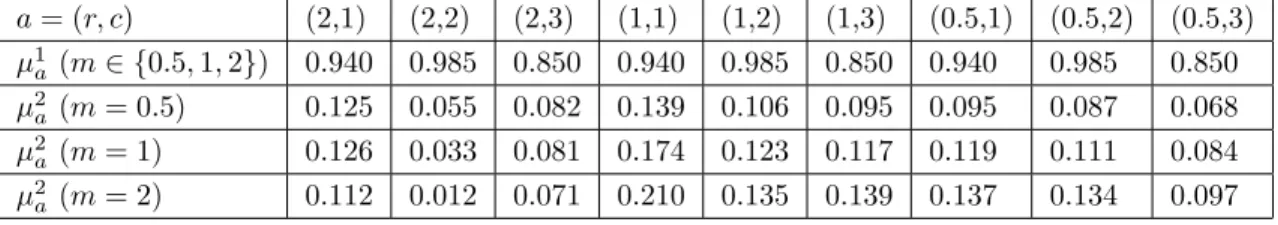
m = 2 . Based on this, the outage event for rate–channel pair (r, c) is defined as log2(1 + h2c,tSINRc,t) < r . Parameters used in the simulations are given in Table2. The given set of parameters corresponds to 9 arms. The expected arm rewards in objectives 1 and 2 are numerically computed by averaging over 5× 10⁷
random samples, and are given Table3. Note that the expected reward in objective 1 does not depend on the channel gain. According to this, the best arms in objective 1 are (2, 2), (1, 2) and (0.5, 2) and the lexicographic optimal arm is (1, 2) for m ∈ {0.5, 1, 2}. However, for m = 2, arm (0.5, 2) is almost as good as arm (1, 2).
on the rate. In all simulations, the time horizon is set to T = 106 and the reported results correspond to the
averages over 50 runs.
Table 2. Simulation parameters. λ ={λc}c∈C denotes the set of channel gain parameters.
C R λ qF P qF N qP U α, β
{1, 2, 3} {2, 1, 0.5} {0.5, 1, 0.5} 0.3 0.3 {0.2, 0.05, 0.5} 1, 3
Table 3. Expected arm rewards for the simulation parameters given in Table2.
a = (r, c) (2,1) (2,2) (2,3) (1,1) (1,2) (1,3) (0.5,1) (0.5,2) (0.5,3) µ1a (m∈ {0.5, 1, 2}) 0.940 0.985 0.850 0.940 0.985 0.850 0.940 0.985 0.850 µ2a (m = 0.5) 0.125 0.055 0.082 0.139 0.106 0.095 0.095 0.087 0.068 µ2a (m = 1) 0.126 0.033 0.081 0.174 0.123 0.117 0.119 0.111 0.084 µ2 a (m = 2) 0.112 0.012 0.071 0.210 0.135 0.139 0.137 0.134 0.097 6.2. Algorithms
In addition to ALEX, we also report the results of the following algorithms:
UCB(δ ): This is the UCB-based single-objective learning algorithm proposed in [25], which uses a slightly different confidence term than UCB1 in [6] and is proven to achieve bounded regret with high probability. Here,
δ denotes the confidence term and is similar to the confidence term of ALEX. In simulations, UCB( δ ) learns
only from objective 1 and the confidence terms of ALEX and UCB( δ ) are set to δ = 0.01 .
Empirical Pareto UCB1 (EP-UCB1): This is the UCB-based multiobjective learning algorithm proposed in [15]. This algorithm aims at learning to select arms from the Pareto optimal arm set in order to minimize the Pareto regret. While it is known that a lexicographic optimal arm is also Pareto optimal, the converse does not generally hold [20].
6.3. Results
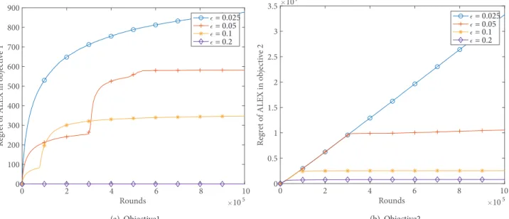
The regrets of ALEX in objectives 1 and 2 over rounds are shown for different ϵ values for m = 1 in Figure1. Based on this, we conclude that the regret decreases in both objectives as ϵ increases. The regret in objective 1 decreases due to the decreasing suboptimality gaps. Moreover for ϵ = 0.1 , 6 out of 9 arms incur no regret in objective 1 and for ϵ = 0.2, all arms incur no regret in objective 1 . The regret in objective 2 decreases because for small values of ϵ, ALEX frequently selects the arm with the highest UCB in objective 1 instead of searching for an approximate lexicographic optimal arm in order to make sure that it learns the best arm in objective 1 well. The sharp increase in the regret in objective 1 corresponds to rounds in which ALEX switches its arm selection rule (from line 8 to line 10 in Algorithm 1).
In addition to the regret, the average reward collected by all of the algorithms by the end of the time horizon is given in Table 4. From this, we observe that for ALEX, increasing ϵ decreases the average reward collected in objective 1 , while increasing the average reward collected in objective 2 for all values of m . This is expected, since as ϵ increases ALEX makes choices from a larger candidate optimal arm set, which includes arms with higher expected rewards in objective 2 but also lower expected rewards in objective 1. We observe
0 2 4 6 8 10 Rounds 105 0 100 200 300 400 500 600 700 800 900
Regret of ALEX in objective
1 = 0.025 = 0.05 = 0.1 = 0.2 (a) Objective1 0 2 4 6 8 10 Rounds 105 0 0.5 1 1.5 2 2.5 3 3.5
Regret of ALEX in objective
2 104 = 0.025 = 0.05 = 0.1 = 0.2 (b) Objective2 Figure 1. Regret of ALEX for different ϵ values in objectives 1 and 2 .
Table 4. Average rewards of the algorithms by round T in objectives 1 and 2 respectively. m ALEX (ϵ = 0.025) ALEX (ϵ = 0.05) ALEX (ϵ = 0.1) ALEX (ϵ = 0.2) UCB(δ) EP-UCB1 0.5 0.983, 0.084 0.963, 0.109 0.942, 0.133 0.940, 0.135 0.984, 0.084 0.963, 0.102 1 0.983, 0.090 0.960, 0.123 0.942, 0.167 0.940, 0.171 0.984, 0.090 0.963, 0.115 2 0.983, 0.095 0.965, 0.137 0.942, 0.201 0.940, 0.207 0.984, 0.095 0.965, 0.126
that when ϵ = 0.025, ALEX performs almost the same as UCB( δ ), which aims at maximizing the total reward in objective 1 . When ϵ = 0.2 , the average reward of ALEX in objective 2 is at least 60% higher than that of UCB( δ ) and at least 32% higher than that of EP-UCB1, while its average reward in objective 1 is only at most 4.47% lower than that of UCB( δ ) and at most 2.59% lower than that of EP-UCB1 for all values of m . These results show the ability of ALEX to tradeoff between the rewards in objectives 1 and 2 by adjusting ϵ. The regrets of all algorithms are compared in Figure2for m = 1 and ϵ = 0.1 . Note that ϵ does not affect the total reward of UCB( δ ) and EP-UCB1 since these algorithms do not take it as input. However, ϵ affects the regrets of these algorithms since it affects the suboptimality gaps of the chosen arms. From the results, we observe that ALEX achieves the smallest regret in objective 2 . Moreover, consistent with the theoretical findings, the regret of ALEX exhibits either logarithmic or bounded growth in both objectives, while the regrets of UCB( δ ) and EP-UCB1 are linear in objective 2. This shows that UCB( δ ) and EP-UCB1 do not have sublinear ϵ lexicographic regret.
Table 5. The fraction of times a 0.1 lexicographic optimal arm is selected.
m ALEX (ϵ = 0.025) ALEX (ϵ = 0.05) ALEX (ϵ = 0.1) ALEX (ϵ = 0.2) UCB(δ) EP-UCB1
0.5 0.343 0.733 0.930 0.956 0.343 0.562
1 0.339 0.660 0.939 0.971 0.341 0.532
0 2 4 6 8 10 Rounds 105 0 50 100 150 200 250 300 350 400 450 Regret in objective 1 ALEX UCB() EP-UCB1 (a) Objective1 0 2 4 6 8 10 Rounds 105 0 0.5 1 1.5 2 2.5 3 3.5 Regret in ob jective 2 104 ALEX UCB() EP-UCB1 (b) Objective2 Figure 2. Regrets of ALEX, UCB( δ ) and EP-UCB1 in objectives 1 and 2 for ϵ = 0.1 .
Finally, the fraction of times a 0.1 lexicographic optimal arm is selected is given for all algorithms in Table 5. Results show that ALEX significantly outperforms UCB( δ ) and EP-UCB1 in selecting approximate lexicographic optimal arms for ϵ = 0.1 and ϵ = 0.2 .
7. Conclusion
In this paper, we proposed a new MAB model called the biobjective MAB and defined the notion of ϵ lexicographic regret. Then, we proposed a learning algorithm called ALEX, and proved that its gap-dependent
ϵ lexicographic regret is bounded with high probability and logarithmic in expectation, and its gap-independent
regret is ˜O(√T ) both with high probability and in expectation. Finally, we modeled multirate multichannel
communication as a biobjective MAB, and investigated how ALEX learns to tradeoff PU interference and SU throughput better than MAB algorithms that are not tailored to learn approximate lexicographic optimal allocations. Possible future application domains for the biobjective MAB include recommendation engines and robotic systems with multidimensional performance metrics.
Acknowledgment
This work was supported by the Scientific and Technological Research Council of Turkey (TÜBİTAK) under Grant No. 116E229. We thank Robin Ann Downey for proofreading the paper and the anonymous reviewers for their suggestions.
References
[1] Lai TL, Robbins H. Asymptotically efficient adaptive allocation rules. Adv Appl Math 1985; 6: 4-22.
[2] Thompson WR. On the likelihood that one unknown probability exceeds another in view of the evidence of two samples. Biometrika 1933; 25: 285-294.
[3] Li L, Chu W, Langford J, Schapire RE. A contextual-bandit approach to personalized news article recommendation. In: 19th International Conference on World Wide Web; 26-30 April 2010; Raleigh, NC, USA. New York, NY, USA: ACM. pp. 661-670.
[4] Tekin C, Liu M. Online learning of rested and restless bandits. IEEE Trans Inf Theory 2012; 58: 5588-5611. [5] Kveton B, Wen Z, Ashkan A, Szepesvari C. Combinatorial cascading bandits. In: 28th Annual Conference on Neural
Information Processing Systems; 7-12 December 2015; Montreal, Canada. Red Hook, NY, USA: Curran Associates, Inc. pp. 1450-1458.
[6] Auer P, Cesa-Bianchi N, Fischer P. Finite-time analysis of the multiarmed bandit problem. Mach Learn 2002; 47: 235-256.
[7] Agrawal S, Goyal N. Analysis of Thompson sampling for the multi-armed bandit problem. In: 25th Annual Conference on Learning Theory; 25-27 June 2012; Edinburgh, Scotland. PMLR. pp. 39.1-39.26.
[8] Gai Y, Krishnamachari B, Jain R. Combinatorial network optimization with unknown variables: Multi-armed bandits with linear rewards and individual observations. IEEE/ACM Trans Netw 2012; 20: 1466-1478.
[9] Combes R, Proutiere A. Unimodal bandits: regret lower bounds and optimal algorithms. In: 31st International Conference on Machine Learning; 21-16 June 2014; Beijing, China. PMLR. pp. 521-529.
[10] Combes R, Proutiere A. Dynamic rate and channel selection in cognitive radio systems. IEEE J Sel Areas Commun 2015; 33: 910-921.
[11] Gai Y, Krishnamachari B, Jain R. Learning multiuser channel allocations in cognitive radio networks: a combi-natorial multi-armed bandit formulation. In: 2010 IEEE Symposium on New Frontiers in Dynamic Spectrum; 6-9 April 2010; Singapore. New York, NY, USA: IEEE. pp. 1-9.
[12] Kveton B, Wen Z, Ashkan A, Szepesvari C. Tight regret bounds for stochastic combinatorial semi-bandits. In: 18th International Conference on Artificial Intelligence and Statistics; 9-12 May 2015; San Diego, CA, USA. PMLR. pp. 535-543.
[13] Chen W, Wang Y, Yuan Y. Combinatorial multi-armed bandit: General framework and applications. In: 30th International Conference on Machine Learning; 16-21 June 2013; Atlanta, GA, USA. PMLR. pp. 151-159.
[14] Chen W, Wang Y, Yuan Y, Wang Q. Combinatorial multi-armed bandit and its extension to probabilistically triggered arms. J Mach Learn Res 2016; 17: 1746-1778.
[15] Drugan MM, Nowé A. Designing multi-objective multi-armed bandits algorithms: a study. In: 2013 International Joint Conference on Neural Networks; 4-9 August 2013; Dallas, TX, USA. New York, NY, USA: IEEE. pp. 1-8. [16] Drugan MM, Nowé A. Scalarization based Pareto optimal set of arms identification algorithms. In: 2014
Inter-national Joint Conference on Neural Networks; 6-11 July 2014; Beijing, China. New York, NY, USA: IEEE. pp. 2690-2697.
[17] Yahyaa SQ, Manderick B. Thompson sampling for multi-objective multi-armed bandits problem. In: 2015 European Symposium on Artificial Neural Networks, Computational Intelligence and Machine Learning; 22-24 April 2015; Brudges, Belgium. Louvain-la-Neuve, Belgium: i6doc.com Publishing. pp. 47-52.
[18] Turgay E, Oner D, Tekin C. Multi-objective contextual bandit problem with similarity information. In: 21st International Conference on Artificial Intelligence and Statistics; 9-11 April 2018; Lanzarote, Spain. PMLR. pp. 1673-1681.
[19] Slivkins A. Contextual bandits with similarity information. J Mach Learn Res 2014; 15: 2533-2568.
[20] Ehrgott M. Multicriteria optimization. 2nd ed. Berlin - Heidelberg, Germany: Springer Science & Business Media, 2005.
[21] Tekin C, Turgay E. Multi-objective contextual bandits with a dominant objective. In: 27th IEEE International Workshop on Machine Learning for Signal Processing; 25-28 September 2017; Tokyo, Japan. New York, NY, USA: IEEE. pp. 1-6.
[22] Tekin C, Turgay E. Multi-objective contextual multi-armed bandit with a dominant objective. IEEE Trans Signal Process 2018; 66: 3799-3813.
[23] Gábor Z, Kalmár Z, Szepesvári C. Multi-criteria reinforcement learning. In: 15th International Conference on Machine Learning; 24-27 July 1998; Madison, WI, USA. San Francisco, CA, USA: Morgan Kaufmann Publishers. pp. 197-205.
[24] Mannor S, Shimkin N. A geometric approach to multi-criterion reinforcement learning. J Mach Learn Res 2004; 5: 325-360.
[25] Abbasi-Yadkori Y, Pál D, Szepesvári C. Improved algorithms for linear stochastic bandits. In: 25th Annual Conference on Neural Information Processing Systems; 12-17 December 2011; Granada, Spain. Red Hook, NY, USA: Curran Associates, Inc. pp. 2312-2320.
[26] Antos A, Grover V, Szepesvári C. Active learning in heteroscedastic noise. Theor Comput Sci 2010; 411: 2712-2728. [27] Stuber GL. Principles of mobile communication. 2nd ed. Norwell, MA, USA: Kluwer, 2001.