OPTIMUM DESIGN OF ANTI-BUCKLING BEHAVIOUR OF THE LAMINATED COMPOSITES BY DIFFERENTIAL EVOLUTION AND SIMULATED ANNEALING ALGORITHMS

İZMİR KÂTİP ÇELEBİ UNIVERSITY  GRADUATE SCHOOL OF NATURAL AND APPLIED SCIENCES

M.Sc. THESIS

DECEMBER 2017

OPTIMUM DESIGN OF ANTI-BUCKLING BEHAVIOUR OF THE LAMINATED COMPOSITES BY DIFFERENTIAL EVOLUTION AND

SIMULATED ANNEALING ALGORITHMS

Thesis Advisor: Asst. Prof. Dr. Levent AYDIN Mehmet AKÇAİR

(Y130105016)

TEMMUZ 2017

İZMİR KÂTİP ÇELEBİ ÜNİVERSİTESİ  FEN BİLİMLERİ ENSTİTÜSÜ

TABAKALI KOMPOZİTLERİN BURKULMA KARŞITI DAVRANIŞLARININ DİFFERENTİAL EVOLUATİON VE SİMULATED ANNEALİNG METODLARI

İLE OPTİMUM TASARIMI

YÜKSEK LİSANS TEZİ Mehmet AKÇAİR

(Y130105016)

Makina Mühendisliği Anabilim Dalı

ACKNOWLEDGMENTS

I would like to express my sincere gratitude to my supervisor Asst. Prof. Dr. Levent Aydın for his advises, guidance, support, encouragement, and inspiration through the thesis. His patience and kindness are greatly appreciated. I have been fortunate to have Dr. Aydın as my advisor and I consider working with his as honor.

I am also grateful to Melih Savran, Ozan Ayakdaş, Aynur Ayvalık, Res. Asst. H. Arda Deveci and Res. Asst.Dr. Burcu Karaca for their support, encouragement and contributions.

I offer sincere thanks to Merve ÇANBAY for her love, support and encouragement. Lastly, the endless gratitude my family for supporting and encouraging me during my undergraduate and postgraduate studies.

TABLE OF CONTENTS

ACKNOWLEDGEMENTS ... IV TABLE OF CONTENTS ... V LIST OF TABLES ... VII LIST OF FIGURES ... IX ABSTRACT ... X ÖZET ... XI CHAPTER 1. INTRODUCTION ... 1 1.1. Literature Survey ... 1 1.2. Objectives ... 3

CHAPTER 2. COMPOSITE MATERIALS ... 4

2.1. Introduction ... 4

2.2. Classification of Composites ... 6

2.3. Applications of Composite Materials ... 11

CHAPTER 3. MECHANICAL ANALYSIS ... 14

3.1. Classical Lamination Plate Theory ... 14

3.2. Buckling Theory of Laminated Composite Plates... 19

CHAPTER 4. OPTIMIZATION ... 22

4.1 Single Objective Optimization ... 23

4.2 Multi Objective Optimization ... 23

4.3. Stochastic Optimization Algorithms ... 24

4.3.1. Differential Evolution Algorithm (DE) ... 24

4.3.2. Simulated Annealing Algorithm (SA) ... 25

4.3.3. Design Approach for Composite Materials ... 27

CHAPTER 5. RESULTS AND DISCUSSION ... 29

5.1 Problem Definition ... 29

REFERENCES ... 46

LIST OF TABLES

Table Page

Table 2.1. Specific modulus and specific strength values of

typical fibers, composites and bulk metals ... 5

Table 2.2. Comparison between plant fibers and E-glass ... 8

Table 2.3. Differences between thermosets and thermoplastics ... 9

Table 2.4. Comparison of conventional matrix materials ... 10

Table 2.5. Advantages and disadvantages of reinforcing fibers... 10

Table 2.6. Application of natural fibers in automotive parts ... 13

Table 4.1. DE and SA parameters used in optimization ... 27

Table 4.2. Design approach for composite materials ... 28

Table 5.1. Optimization problems ... 30

Table 5.2A. The elastic properties of different reinforced composite materials ... 34

Table 5.2B. The elastic properties of different Glass/Epoxy composites ... 35

Table 5.2C. The elastic properties of different Graphite/Epoxy composites ... 36

Table 5.3. Composite plate load cases ... 36

Table 5.4. Verification of objective function and comparison of optimum stacking sequences design in term of buckling for 64-layered symmetric and balance Graphite/Epoxy laminates with 45 degree increment. ... 37

Table 5.5. Effect of different degree increments for the critical buckling load factor values based on DE. (D1, D 2, D3, D4, D5, corresponds to 1, 5, 15, 30, 45 degree increments, respectively). ... 38

Table 5.6. Optimum stacking sequence designs for different load cases and degree increments based on DE. (D1, D2, D3, D4, D5 corresponds to 1, 5, 15, 30, 45 degree increments, respectively) ……….… 39

Table 5.7. Effect of different reinforced composites on critical

buckling load factor with different degree increments based on DE. (D1, D 2, D3, D4, D5, corresponds to 1, 5, 15, 30, 45

degree increments, respectively). ... 40

Table 5.8A. Effect of different reinforced composite materials on optimum stacking sequence designs with different

degree increments based on DE. (D1, D 2, D3, corresponds to

1, 5,15 degree increments, respectively) ... 41 Table 5.8B. Effect of different reinforced composite materials on

optimum stacking sequence designs with different degree increments based on DE. (D4, D5 corresponds to

30, 45 degree increments, respectively) ... 42 Table 5.9. Different Glass/Epoxy composites critical buckling load factor

values and corresponding stacking sequences designs

based on DE (D5 (90  90) 45 degree increments) for LC1. ... 43 Table 5.10. Different Graphite/Epoxy composites critical buckling load factor

values and corresponding stacking sequences designs

LIST OF FIGURES

Figure Page

Figure 2.1. Variation of specific strength with time for

different materials ... 5

Figure 2.2. Types of composites based on reinforcement shape ... 6

Figure 2.3. Cost per weight comparison between glass, graphite and natural fibres ... 8

Figure 2.4. Plant fibre reinforced polimers (PFRPs) accounted for 1.9% of the 2.4 million tonne EU FRP market in 2010 ... 11

Figure 2.5. Use of fiber-reinforced polymer composites in Boing 787 ... 12

Figure 3.1. Composite plate subject to in-plane loading ... 15

Figure 3.2. Coordinate locations of plies in a laminate ... 15

Figure 3.3. Representation of normal and shear force-moment resultants ... 17

Figure 3.4. Representation of simply supported rectangular plate ... 20

Figure 4.1. Flowchart of the DE algorithm ... 25

Figure 4.2. Flowchart of the SA algorithm ... 26

Figure 5.1. Laminated composite subjected to in-plane loads ... 29

Figure 5.2. Variation of critical buckling load factors with different degree increments. ... 38

ABSTRACT

OPTIMUM DESIGN OF ANTI-BUCKLING BEHAVIOUR OF THE

LAMINATED COMPOSITES BY DIFFERENTIAL EVOLUTION AND

SIMULATED ANNEALING ALGORITHMS

Laminate composites can be used quite naturally in automotive, marine, aviation and other engineering branches. Determination of buckling load capacity under in-plane composite loads of composite plates is very important for the design of composite structures. In this thesis, Differential Evolution (DE) and Simulated Annealing (SA) are utilized for optimal stacking sequence of a laminated composite plate, which is simply supported on four edges and is subjected to biaxial in-plane compressive loads. The optimization problem parameters are defined as

(i) Objective function: critical buckling load factor,

(ii) Constraints: symmetric and balanced structure, thin plate assumption, specially orthotropic material, discrete search space,

(iii) Design variables: fiber orientation angles of lamina.

The laminated composite plate under consideration is 64- ply laminate made of graphite/epoxy. The fiber angles are integers varying between -90 and 90 (90  90) with different degree increments in the laminate sequence.

In cases where the angle variation are continuous and discrete, the optimization results are compared. In addition, the optimization methods used in similar optimization studies in the literature and the results obtained under the thesis (based on DE and SA) are also compared. The critical buckling loads are maximized for the factors of load case and plate aspect ratio, and are compared with published results. Moreover, critical buckling load factor has been investigated for the materials Boron/Epoxy, Graphite/Epoxy, Carbon/Epoxy, Kevlar/Epoxy, S2 Glass/Epoxy, Fiberite/HyE9082A, S-Glass/Epoxy, E-Glass/Epoxy,

Flax/Epoxy, E-Glass/Polyster, Alfa/Polyester and Flax/Polypropylene. As a result, it has been found that the parameters load, load ratio and plate aspect ratio are effective for optimization of the critical buckling load factor that increases buckling resistance of laminated composites. It is also observed that the DE method shows better computational performance than SA.

ÖZET

TABAKALI KOMPOZİTLERİN BURKULMA KARŞITI

DAVRANIŞLARININ DIFFERENTIAL EVOLUTION VE SIMULATED

ANNEALING METOTLARI İLE OPTİMUM TASARIMI

Lamina kompozitler, otomotiv, denizcilik, havacılık ve diğer mühendislik dallarında kullanılabilmektedir. Kompozit plakaların düzlem içi bası yükleri altında burkulma yük kapasitesinin belirlenmesi, tabakalı kompozit yapıların tasarımı için çok önemlidir. Bu tezde, çift eksenli düzlem içi bası yüklerine maruz ve dört taraftan basit mesnetli kompozit plakaların burkulma karşıtı davranışlarının optimum tasarımı karşılaştırmalı olarak Differential Evoluation ve Simulated Annealing metotları ile yapılmıştır. Optimizasyon problemine ait parametreler aşağıdaki şekilde tanımlanmıştır:

(i) Amaç fonksiyonu: Kritik burkulma yük faktörü

(ii) Kısıtlar: Simetrik ve balans yapı, ince plaka varsayımı, özellikli ortotropik malzeme, ayrık arama uzayı,

(iii) Tasarım Değişkenleri: Laminaya ait fiber oryantasyon açıları.

Ele alınan tabakalı kompozitler 64 tabakalı Grafit/Epoksi malzemeden oluşmuştur. Fiber açıları [-90, 90] aralığında değişen şekilde tam sayılı olarak alınmıştır; bu tam sayılı artış miktarları sabit değildir.

Açı artırımının sürekli ve ayrık olduğu durumlarda optimizasyon sonuçlarının

karşılaştırılması yapılmıştır. Buna ek olarak literatürdeki benzer optimizasyon çalışmalarında kullanılan optimizasyon yöntemleri ile tez kapsamında elde edilen sonuçlar (DE ve SA

tabanlı) kıyaslanmıştır. Kritik burkulma yük faktörü, faklı yük ve plaka (en boy) oranına bağlı olarak maksimize edilip, önceki çalışmalarla sonuçları karşılaştırılmıştır. Ayrıca

Boron/Epoksi, Grafit/Epoksi, Karbon/Epoksi, Kevlar/Epoksi, S2 Glass/Epoksi, Fiberit/HyE9082A, S-Glas/Epoksi, E-Glas/Epoksi, Keten/Epoksi, E-Glas/Polyester, Alfa/Polyester ve Flax/Polipropilen malzemeler için kritik burkulma yük faktörleri

hesaplanmıştır. Sonuç olarak, tabakalı kompozitlerin burkulma direncini artıran, burkulma yük faktörü optimizasyonu için; yük, yük oranı ve plaka en-boy oranı parametrelerinin etkin olduğu gözlenmiştir. Bunun yanında DE’nin hesaplama performansının SA’ya göre daha iyi olduğu gözlenmiştir.

CHAPTER 1

INTRODUCTION

1.1

Literature Survey

In recent years, fiber-reinforced composite materials are utilized in automotive, marine, aerospace and other engineering applications because of their high strength and high stiffness to weight ratio. Optimum designs of composite laminates subjected to uniaxial and biaxial compressions are very important. Some examples of their implementations are strong and rigid aircraft frames, lightweight, sports equipment, composite drive shafts and suspension components, pressure vessels and high-speed flywheels with developed energy storage capabilities. The anisotropic structure of fiber-reinforced composites provides a unique opportunity to tailor features such as laminate stacking sequence, thickness and fiber orientation according to design requirements for a particular application. As a result, the design of composite materials can be optimized over different objective functions and design variables (Pelletier & Vel, 2006).

Many optimization researches have been studied for composite structures. Researchers have investigated optimization for the minimum weight (Schmit & Farshi, 1973), stiffness (Kam, 1991), strength (Kim et al., 1998; Cheol W. Kim & Hwang, 1999). For dynamic analysis, Bert (1977) and Adali and Verijenko (2001) performed the optimization for the maximum fundamental frequency. The composite laminated plates are often subjected to uniaxial and biaxial compressions. For thin and wide composite plates subjected to loads in the compression plane, buckling should be considered as a critical failure mode. The buckling load capacity of composite plates under in-plane pressures is very important for the design of composite structures. Therefore it is critical to investigate buckling-post buckling behaviors of the laminated composite structures satisfying high buckling resistance in many engineering applications such as aircraft, automobile and ships design. For this reason, many researchers have attempted to solve design problems of composite structures including

buckling conditions; Chao et al., (1975) initiated the buckling load optimization for the uniaxial compression. Hu and Lin (1995) used linear programming method, while Haftka and Walsht (1992) used the Branch and Bound method to find the optimum design, and calculated the optimal fiber orientation for the uniaxial compressed plate and shell by traditional optimization techniques. Due to the inherent features of anisotropic composites and from the view point of mathematical optimization, the most challenging design problems occur in composite structures engineering. Therefore, conventional techniques such as Lagrange Multipliers, Simplex are not sufficient or limited to solve the problem having discrete search spaces (Aydin & Artem, 2011). In these cases, the use of stochastic optimization methods such as Genetic Algorithms (GA), Generalized Pattern Search Algorithm (GPSA), Differential Evolution (DE) and Simulated Annealing (SA) are appropriate (C. W. Kim & Lee, 2005). Karakaya & Soykasap (2009) maximized the critical buckling load factor for various design cases in order to design the optimum composite plates with conventional fiber angles by GA method. In the literature, optimization of stacking sequence order of laminate composites is also considered to maximize buckling load factor with other stochastic optimization methods such as GPSA (Karakaya & Soykasap 2009), SA (Pai et al., 2003), Scatter Search (Erdal & Sonmez, 2005), Tabu Search (Mohan Rao & Arvind, 2005), Ant Colony Optimization (ACO) (Aymerich & Serra, 2008), (Sebaey et al., 2011) algorithms. Optimization of buckling load of composite laminate subjected to mechanical loading alone as well as optimization of thermal buckling of laminated composite laminates have been investigated in the literature. The problem of optimization of thermal buckling of laminate composite plates in aeronautical structures, which require components that can withstand external environmental loads without loss of stability, is solved under strain and creep constraints using evolutionary strategies, according to a Guided Random Search method by Spallino & Thierauf (2000). The other study, thermal buckling optimization of laminated plates exposed to evenly distributed temperature loads was investigated to obtain the best fiber orientation designs with maximum critical temperature capacity of the laminated plates using the Modifiable Orientation (MFD) method (Topal & Uzman, 2008). The optimization of laminates and sandwich plates according to buckling load and thickness has been done by using Evolutionary algorithms (Di Sciuva et al., 2003)

Regarding of these facts, in this study, DE and SA are used for optimal stacking sequence of a 64-layer composite laminated plate made of graphite–epoxy, which is simply supported on four edges and subject to biaxial in-plane compressive loads. The main purpose of this thesis is to utilize the optimization algorithms for the critical buckling load factor that is taken as objective function. Fiber orientations are selected as design variables. The critical buckling load factor is maximized for various loading cases and plate aspect ratio combinations and compared to the results published in Karakaya & Soykasap (2009). Both algorithms are compared for their effectiveness. The optimization application is done using Nminimize solver including DE and SA algorithms at Mathematica (The Mathworks Inc 2009).

Finally, the design and optimization for the critical buckling load factor was also performed to see the effect of different fiber and matrix materials on the stacking sequences by DE method only.

1.2. Objectives

The main objectives of this thesis can be listed as follows:

1) To determine the best fiber angles of 64-layered carbon/epoxy composites for various plate aspect ratios with different compressive in-plane loads to withstand buckling

2) To compare optimum values of the objective function (buckling load factor) in the laminated composite plates for different design cases.

3) To optimize critical buckling load factor by different stochastic optimization methods which are Differential Evolution and Simulated Annealing

4) To show applicability of discrete fiber orientation designs instead of continuous ones.

5) To investigate critical buckling load factor in terms of different composite materials in the literature.

CHAPTER 2

COMPOSITE MATERIALS

2.1 Introduction

In general, a composite is a structural material consisting of two or more components joined together at the macroscopic level and insoluble in each other. The components are separated into two; one is called reinforcement and the other is called the matrix. The reinforcing material may be in the form of fibers, particles, sheets or different geometries. The matrix materials are generally in continuous nature. Some examples of composite systems are steel-reinforced concrete and epoxy glass fiber reinforced, etc. (Kaw 2006).

The integration of materials with advanced material properties to create a new material system is constantly being implemented throughout history. For example, the ancient Egyptian workers included the minced straws in the bricks, improving the structural integrity during the construction of the pyramids. Eskimos made strong frosty houses using moss. Japanese samurai warriors have used laminate metal in sword tattoos to provide the desired material properties. In the 20th century, civil engineers placed iron into the cement and produced a well-known composite material, namely reinforced concrete. It can be argued that the modern times of composite materials started with glass fiber polymer matrix composites during the Second World War (Vinson & Sierakowski 2004).

Many fiber reinforced materials provide a better combination of strength and modulus than many conventional metallic materials, since fiber-reinforced composite materials have specific properties that have low density, high specific modulus (ratio between the young modulus and the density) and specific strength (ratio between strength and density). In addition, fatigue strength and tolerance to fatigue damage of many laminated composites are quite good. For this reason, fiber-reinforced materials have emerged as an important class of structural materials, and they are considered to be metals in many of the critical components in terms of weight in aviation, automotive and other industries(Mallick, 2007).

Figure 2.1 shows the comparison of fibers and composites with other conventional materials in terms of specific strength on an annual basis.

Figure 2.1 : Variation of specific strength with time for different materials. (Source: Kaw 2006)

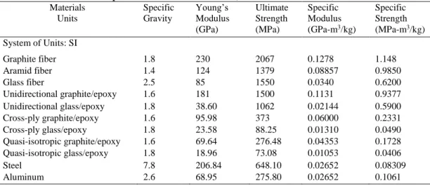
In Table 2.1, specific gravity, Young’s moduli, ultimate strength, specific moduli and strength values are given for many widely used isotropic metals and composite materials (Kaw 2006).

Table 2.1 : Specific modulus and specific strength values of typical fibers, composites and bulk metals (Source: Kaw 2006)

Materials Units Specific Gravity Young’s Modulus (GPa) Ultimate Strength (MPa) Specific Modulus (GPa-m3_/kg) Specific Strength (MPa-m3_/kg) System of Units: SI Graphite fiber 1.8 230 2067 0.1278 1.148 Aramid fiber 1.4 124 1379 0.08857 0.9850 Glass fiber 2.5 85 1550 0.0340 0.6200 Unidirectional graphite/epoxy 1.6 181 1500 0.1131 0.9377 Unidirectional glass/epoxy 1.8 38.60 1062 0.02144 0.5900 Cross-ply graphite/epoxy 1.6 95.98 373 0.06000 0.2331 Cross-ply glass/epoxy 1.8 23.58 88.25 0.01310 0.0490 Quasi-isotropic graphite/epoxy 1.6 69.64 276.48 0.04353 0.1728 Quasi-isotropic glass/epoxy 1.8 18.96 73.08 0.01053 0.0406 Steel 7.8 206.84 648.10 0.02652 0.08309 Aluminum 2.6 68.95 275.80 0.02652 0.1061

2.2. Classification of Composites

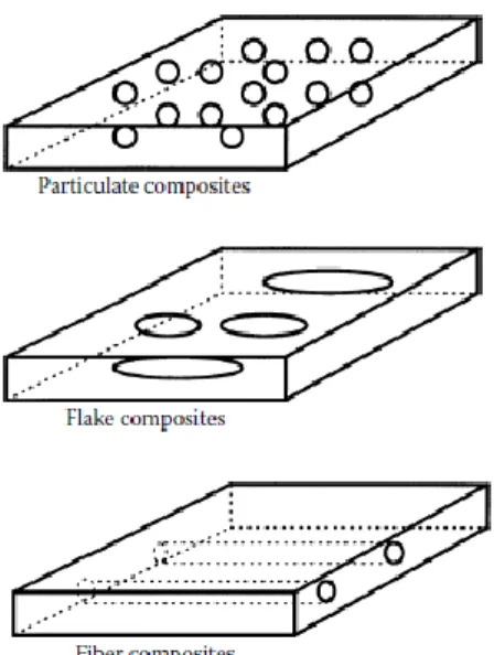
Composites can be classified either the geometry of the reinforcement material such as particulate, flake, and fibers (Figure 2.2) or the type of matrix such as metal, ceramic, carbon and polymer.

Figure 2.2 : Types of composites based on reinforcement shape. (Source: Kaw 2006)

Particulate composites comprise inserted particles in matrices such as ceramic and alloys. Use of aluminum particles in rubber; silicon carbide particles in aluminum; and common examples of cement-particle composites for making gravel, sand and concrete. Fiber reinforced laminated composite materials comprise thin or flat fiber reinforced matrices. In addition, they can be used as classical flake materials in glass, graphite, mica, aluminum and silver composites. The main advantages of structural use of flake composites are out-of-plane bending modulus, high strength and low cost. On the other hand, these composites have some drawbacks. For example, stamps cannot be easily guided and only a few materials are suitable for use.

Composite materials include a continuous matrice and long or short fibers. The fibers are generally anisotropic; Glass, graphite, boron, kevlar, carbon, and aramid are the most common examples of fibers. Matrix samples of resins such as epoxy, vinylester, polyester are generally isotropic. In continuous fiber matrix composite materials

unidirectional or woven fiber laminates can be utilized and they are also stacked on top of each another at different make up a multidirectional laminate (Kaw 2006). The most commonly used advanced composites are polymer matrix composites (PMCs) comprising of a polymer such as polyester, epoxy and urethane, reinforced with thin-diameter fibers such as glass, graphite, boron, fiberite and aramid. These composites are preferred due to their low cost, high strength and simple production principles. The principal disadvantages of PMCs are low operating temperatures, high thermal and moisture expansion coefficients, and low elastic properties in certain directions. Glass and graphite fibers in the polymer matrix composite are used in a extensive range of engineering applications. Graphite fibers are used more frequently in high-modules and high-strength applications such as aircraft equipment etc. Its own low thermal expansion coefficient and high fatigue strength. The disadvantages are high cost, low impact resistance, and high electrical conductivity. Particularly high cost limits the use of his material without special applications. In order to overcome this disadvantage, glass fibers are used together with graphite in many constructions. In this way both good structural stability and low cost can be achieved. Moreover to low cost, glass fiber has advantages that high strength and chemical resistance, good insulation properties. The disadvantages are low elastic modulus, weak adhesion to polymers, high specific gravity, abrasion resistance (reduces tensile strength) and low fatigue strength. The main types of glass fibers are E-glass (fiberglass), S-glass which is used for electrical and structural applications, and the higher silica content and the high temperature power. Other glass fiber types include C-glass (corrosion), R-glass for structural applications, D-glass (Dielectric) for applications with low dielectric constants, A-glass (Appearance) for use in surface treatment.

Natural fibers offer economical, technical and ecological advantages compared to synthetic fibers in reinforced polymer composites. Due to the relatively abundance, low density, high specificity and eco-friendly profile of plant fibers such as linen, hemp and jute, natural fibers have been preferred as synthetic fibers, particularly E-cama alternative reinforcing materials (Shah et al., 2012; Wambua et al., 2003; Faruk et al., 2012). Comprasion of different properties between natural fibers and E-glass fiber are indicated in Table 2.2.

Table 2.2: Comparison between plant fibers and E-glass (Source: Shah D et al. 2013) Properties Plant fibres E-Glass fibre

Economy Annual global production (tonnes) 31,000,000 4,000,000 Distribution for FRPs in EU (tonnes) Moderate (40,000) High (600,000)

Technical Density (g cm-3_{) Low (~1.35-1.55) High (2.66)}

Tensile stiffness (GPa) Moderate (~30-80) Moderate (73) Tensile strength (GPa) Low (~0.4-1.5) Moderate (2.0-3.5) Tensile failure strain (%) Low (~1.4-3.2) Low (2.5) Specific tensile stiffness (GPa/g cm-3_{) Moderate (~20-60) Low (27)}

Specific tensile strength (GPa/g cm-3_{) Moderate (~0.3-1.1) Moderate (0.7-1.3)}

Abrasive to machines No Yes

Ecological Energy consumption (MJ/kg of fibre) Low (4-15) Moderate (30-50)

Renewable source Yes No

Recyclable Yes Partly

Biodegradable Yes No

Toxic (upon inhalation) No Yes

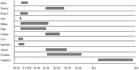
In addition to being eco-friendly, natural fibers are lower cost than synthetic fibers. The cost of some natural fibers, glass and graphite fiber are shown in Figure 2.3.

Figure 2.3: Cost per weight comparison between glass, graphite and natural fibres (Dittenber et al. (2012))

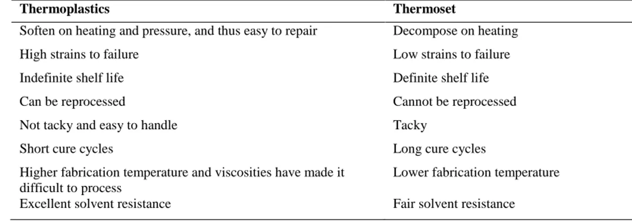
There are various polymers used in thermoset-classified (epoxy, polyester, phenolic and polyamide) and thermoplastic (polyethylene, polystyrene, polyether-ether-ketone (PEEK) and polyphenylene sulfide (PPS)) advanced polymer composites. Thermoset polymers attached to strong covalent bonds are insoluble and infused after curing; Thermoplastics contain weak van der Waals bonds and can therefore be formed at high pressures and high temperatures. The variation between thermosets and thermoplastics are shown in Table 2.3 (Kaw 2006).

Table 2.3: Differences between thermosets and thermoplastics (Source: Kaw 2006)

Thermoplastics Thermoset

Soften on heating and pressure, and thus easy to repair Decompose on heating

High strains to failure Low strains to failure

Indefinite shelf life Definite shelf life

Can be reprocessed Cannot be reprocessed

Not tacky and easy to handle Tacky

Short cure cycles Long cure cycles

Higher fabrication temperature and viscosities have made it difficult to process

Lower fabrication temperature Excellent solvent resistance Fair solvent resistance

Epoxy resins are the most widely used thermosetting PMC, but are more expensive than other polymer matrices.

Epoxy matrices have some advantages such as high strength, low viscosity and low flow rate which allow the fibers to be well wetted and to lessen the tendency to achieve low evaporation, low shrinkage, and thus high tendency to bond large shear stresses during hardening of the fibers during processing and between epoxy and reinforcement. They can be used for a wide variety of engineering applications. Metal matrix composites (MMC), are carbon (graphite), boron or ceramic fiber reinforced metals or alloys (aluminum, magnesium, titanium and copper). Materials are often used to provide advantages such as steel and aluminum on metals. The most important features of these composites are

i) low coefficient of thermal expansion, ii) ii) high specific modulus and strength, iii) iii) low density

Ceramic matrix composites (CMCs), are ceramic fiber reinforced ceramic matrices (aluminum calcium, silicon carbide, aluminum oxide, glass-ceramic, silicon nitride). The main advantages of CMCs are high hardness, strength, high service temperature limits for ceramics, low density and chemical inertness. However, ceramic matrix composites have low fracture toughness.

Carbon-carbon composites (C / C) contain carbon fiber reinforcement in the graphite or carbon matrix. Such composites have high temperature, low thermal expansion and high strength properties at high density. On the other hand, disadvantages of C / C composites are high cost, low shear strength and sensitivity to high temperature oxidation. Typical properties of conventional matrix materials are

given in Table 2.4 and Table 2.5 in comparison with each other, with each matrix type and fiber having advantages and disadvantages.

In this study, graphite/epoxy composite (T300/5208) is considered as a main design material.

Table 2.4 : Comparison of conventional matrix materials (Source: Daniel & Ishai 1994)

Property Metals Ceramics Polymers Bulk Fibers Tensile strength + - ++ v Stiffness ++ v ++ - Fracture toughness + - v + Impact strength + - v + Fatigue endurance + v + + Creep v v ++ - Hardness + + + - Density - + + ++ Dimensional stability + v + - Thermal stability v + ++ - Hygroscopic sensitivity ++ v + v Weatherability v v v + Erosion resistance + + + - Corrosion Resistance - v v +

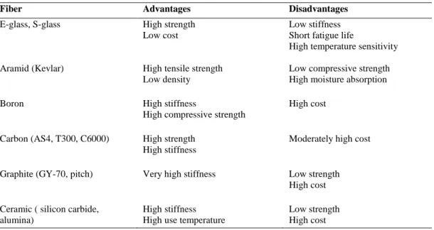
Table 2.5: Advantages and disadvantages of reinforcing fibers (Source: Daniel & Ishai 1994)

Fiber Advantages Disadvantages E-glass, S-glass High strength

Low cost

Low stiffness Short fatigue life

High temperature sensitivity Aramid (Kevlar) High tensile strength

Low density

Low compressive strength High moisture absorption

Boron High stiffness

High compressive strength

High cost

Carbon (AS4, T300, C6000) High strength High stiffness

Moderately high cost

Graphite (GY-70, pitch) Very high stiffness Low strength High cost

Ceramic ( silicon carbide, alumina)

High stiffness High use temperature

Low strength High cost

2.3 Applications of Composite Materials

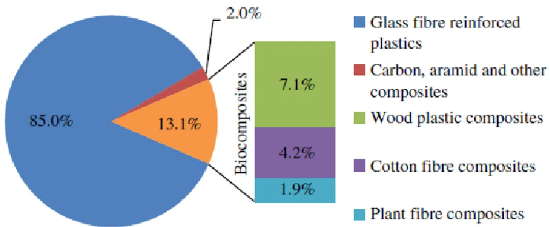
Fiber-reinforced polymer composites are utilized in various engineering fields since they have better strength and modulus than conventional monolithic metal materials. Application areas of composite materials; Aircraft, automotive, space, sporting goods, boat and marine, medical industry and military. Figure 2.4 shows the relative market share of EU for synthetic and natural fiber composites, and it appears that the most used fiber is glass in the composite sector. Composite materials such as aramid, carbon are only used in special applications for their high prices. For example, these composites are frequently utilized in military and commercial aircraft, as these materials can provide both light weight and strength.

Fig. 2.4: Plant fibre reinforced polimers (PFRPs) accounted for 1.9% of the 2.4 million tonne EU FRP market in 2010 (Source: Carus, 2011)

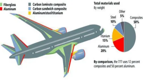
A lighter aircraft is less burning fuel, so weight reduction is important for military and commercial aircraft. Figure 2.5 shows the usage of composite materials in different components of the Boeing 787 aircraft. Carbon fibers were introduced to the industry in the 1970s, and carbon epoxy composites were the main material in many aerospace structure components. Utilizing sustainable composite structures for the builder has improved the performance and leads to develop new structure of engineering materials. For instance, F-22 fighters have 25% carbon fiber reinforced polymers by weight; other materials are titanium (39%) and aluminum (16%). Almost all are made from carbon fiber reinforced polymers because of stealth planes, special coatings, design properties which simplify the reflection from radar and thermal radiation. Furthermore, it is used in military and commercial helicopters to carry many fiber reinforced polymers, luggage compartments, cornices, vertical wings, tail rotor spars, and the like (Mallick 2007).

Figure 2.5: Use of fiber-reinforced polymer composites in Boing 787 (Source: Bintang 2011)

The other important application for composite materials is the automotive industry. The body, chassis and engine combination are the three key elements in the automotive industry. Because of its higher cost, carbon fiber may not be preferred If it is compared to E-glass fiber. Especially, door panels and hood like body composition requires high hardness and damage tolerance. Hence the laminated composites utilized in the related components are made up of E-glass fiber-sheet metal molding compound materials. For the chassis element, the main structural implementation of composites material is the rear leaf spring. The usage of unileaf E-glass/epoxy springs instead of multi-sloping steel springs provides a weight reduction of about 80%.

Other chassis components, such as wheels and drive shafts, have been successfully tested, but are manufactured in limited quantities. The implementation of laminated composites on the engine component was not as achieve as the other component. (Mallick 2007).

Todays, the use of natural fibers as reinforcement for engineering applications instead of glass fibers in composites has gained popularity due to increased environmental concerns and the need to develop sustainable materials. Approximately 315,000 tonnes of natural fibers were used as reinforcements in composites in the European Union (EU) in 2010, which was established for 13% of total reinforcing materials (glass, carbon and natural fibers) in fiber reinforced composites (Yan et al., 2014). In commercial practice, more than 95% of the PFRPs produced in the EU are used for

non-structural automotive parts. Table 2.6 shows the use of natural fibers in automotive parts. Table 2.6 shows the usage of natural fibers in the automotive sector. Table 2.6: Application of natural fibres in automotive parts (Source: Bos, 2004).

Next to automotive applications, natural fibers generally are utilized for interior parts such as doors and instrumental panels; for bridges, beams, ceiling panels and for construction and infrastructure applications; sporting goods such as tennis rackets, boat hulls, bicycle frames and canoes; furniture and consumption goods; packages, boxes, bags, chairs, tables, helmets, ironing tables.

CHAPTER 3

MECHANICAL ANALYSIS

In recent years, material scientists and many engineers have experienced the design and behavior of isotropic materials that contain the relation of most metals and pure polymers. Anisotropic materials are preferred to other materials. Especially composite materials have ended up with a materials revolution and they are required some anisotropic behavior based new information.

Fiber-reinforced composite materials use in comparison with conventional materials in application. Moreover, long fibers results use in material that has stiffness-to-density ratio and/or higher strength-stiffness-to-density ratio than the other materials and tailor the fiber orientations according to the specific geometry, applied load and the environment are uniquely adapted opportunity. Also, mainly low-cost mass production and the use of short fibers for fiber reinforced composites used in the system and makes it more competitive and superior to metal and plastic alternative materials. Therefore, with the use of composite materials, an engineer is not just a material selector but a material designer at the same time (Vinson 2004). Furthermore, laminated composites materials reinforced by the fibers are orthotropic and inhomogeneous. For this reason, investigation of mechanical behavior for them are complicated than those of traditional homogeneous and isotropic materials such as aluminum and steels (Mallick 2007).

3.1 Classical Laminated Plate Theory

The theory is applied to define mechanical behavior of laminated composites and is only used under the following assumptions

 Laminae is orthotropic and homogeneous.

 Each lamina is elastic and bounded each other perfectly.

 The thickness of the laminate composite is thinner and the thickness of the composite plate is much less than the edge dimensions.

 The loads are applied only on the plane of the laminate and the laminated composite (excluding the edges) is subjected to plane stress (σzτxz=

τyz=0).

 The displacements are a small contrast to the thickness of the laminate and are continuous throughout the laminate.

 In-plane displacement components in x and y can be written as linear functions of z.

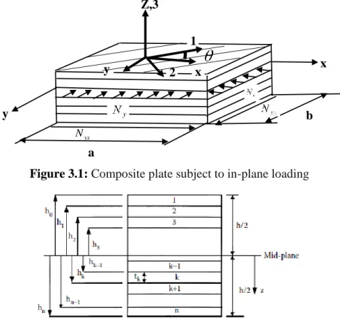
 Transverse shear strains (γxz and γyz ) are ignorable because a line straight and perpendicular to the middle surface maintains the condition along the deformation. Considered thin laminated composite plate exposed mechanical in-plane loading (Nx,

Ny) in this thesis is shown in Figure 3.1. Global coordinates of the laminated material are defined as x, y and z. A layer-wise material is represented by the coordinate system 1, 2 and 3; the fiber orientation angle with x-axis denotes , n is the number of layers and h is total thickness (see Figure 3.2.)

Figure 3.1: Composite plate subject to in-plane loading

Figure 3.2:Coordinate locations of plies in a laminate (Source: Kaw 2006) yx N y a Ny x Nx x y Z,3 2 1 Z b

In most structural applications, composite materials are used as thin laminates loaded onto the plane of the laminate. As a result, it can be assumed that composite laminates are under planar stress conditions and all stress components in the out-of-plane direction (3-way) are zero.

According to Classical Laminated Plate Theory, the relation between stress and strain for each layers can be expressed as

k xy y x o xy o y o x k k xy y x z Q Q Q Q Q Q Q Q Q                                                              66 26 16 26 22 12 16 12 11 (3.1)

where [Q_ij ]k are the elements of the transformed reduced stiffness matrix, [

o





The transformed reduced stiffness matrix [Q_ij ] given in Equation (3.1) can be written as in the following form

2 2 66 12 4 22 4 11 11 Q c Q s 2(Q 2Q )s c Q     ) ( ) 4 ( _{11 22 66} 2 2 ₁₂ 4 4 12 Q Q Q s c Q c s Q      2 2 66 12 4 22 4 11 22 Q s Q c 2(Q 2Q )s c Q     c s Q Q Q sc Q Q Q Q₁₆ ( ₁₁ ₁₂2 ₆₆) 3 ( ₂₂  ₁₂ 2 ₆₆) 3 3 66 12 22 3 66 12 11 26 (Q Q 2Q )cs (Q Q 2Q )sc Q       ) ( ) 2 2 ( _{11 22 12 66} 2 2 ₆₆ 4 4 66 Q Q Q Q s c Q c s Q       (3.2-a-f)

where ccos





Q

12 21 1 11 1











where ₁₂ is major Posion’s ratio, E1 is longitudinal elastic modules,E2is transverse

elastic modules, G₁₂ is shear modules.

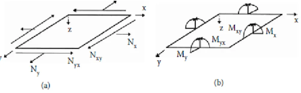
Figure 3.3: Representation of normal and shear force-moment resultants (Source: Kaw 2006)

Applied normal force resultantsN_x,N_y, shear force resultantN_xy (per unit width) and moment resultants M_x,My and Mxy on a laminate (see Fig. 3.3) are

expressed as:                                                     xy y x xy y x xy y x B B B B B B B B B A A A A A A A A A N N N       66 26 16 26 22 12 16 12 11 0 0 0 66 26 16 26 22 12 16 12 11 (3.8)                                                     xy y x xy y x xy y x D D D D D D D D D B B B B B B B B B M M M       66 26 16 26 22 12 16 12 11 0 0 0 66 26 16 26 22 12 16 12 11 (3.9)

The matrices [A], [B] and [D] can be defined as

     n k ij k k k ij Q h h A 1 1 ) ( )] [( , i, j 1,2,6 (3.10)      n k ij k k k ij Q h h B 1 2 1 2 ) ( )] [( 2 1 , i, j 1,2,6 (3.11)      n k ij k k k ij Q h h D 1 3 1 3 ) ( )] [( 3 1 , i, j 1,2,6 (3.12)

The [A], [B], and [D] matrices are called the extensional, coupling, and

bending stiffness matrices, respectively. Equation 3.8 and Equation 3.9 can be combined as in the following form including 6 unknowns:

(3.13)

Matrix [A] interrelates the resultant in-plane forces to the in-plane strains, matrix [B] represents a coupling between stretching and bending of the laminate and finally [D] gives the relation between bending moments and the plate curvatures (Kaw 2006).

In this case, for an angled lamina the transformation formulation between the local and global stresses can be expressed as:

 

By a similar manner, the relation between local and global strains becomes:

   

where

 

 

and [T] transform matrix,

                                                             xy y x xy y x xy y x xy y x D D D B B B D D D B B B D D D B B B B B B A A A B B B A A A B B B A A A M M M N N N       0 0 0 66 26 16 66 26 16 26 22 12 26 22 12 16 12 11 16 12 11 66 26 16 66 26 16 26 22 12 26 22 12 16 12 11 16 12 11

              2 2 2 2 2 2 2 2 ] [ s c sc sc sc c s sc s c T c cos





3.2 Buckling Theory of Laminated Composite Plates

Assuming that the composite plate is loaded byN_x, N_yand N_xy in-plane compressive loads, where  is a scalar amplitude parameter and simply supported on four sides, the governing differential equation for the buckling behavior of the plate, thinking the classical plate theory, is;







where D11, D12, D22, D66 are the terms of bending stiffness’s, wis the vertical displacement and it is given by

b y n a x m A y x w mn n m   sin sin ) , ( 





forces are defined as follows: x N  N₀ N_y kN₀ (3.20) where k= y x N N

The boundary conditions for simply supported rectangular plate (see Figure 3.4) can be written as in the following form:

w x( , 0)0, w x( , b)0, w(0, y)0, w(a, y) 0 , (3.21) Mxx( , 0)x 0,Myy( , )x b 0, Myy(0, )y 0, Mxx( , )a y 0 (3.22)

Figure 3.4 Representation of simply supported rectangular plate

(Adapted from: Reddy 2004)

With the substitution of Eq. 3.19 into Eq. 3.18, and solving eigen function problem, buckling load factor expression can be obtained as





A considerable point is that D16 and D26 do not appear in Eq. 3.19 and 3.20,

because they are zero for a specially orthotropic laminate and they are small check against to the other Dij’s for a symmetric laminate with a number of laminas of ±θ ply angles in sequence.

The laminate buckles into m and nhalf-waves in the x and y directions, respectively, when the magnitude parameter approaches a critical value of _b

(Spallino & Thierauf, 2000). The critical buckling load factor  limits the maximum _cb load which the laminate can endure without buckling and it is the smallest value of  b under suitable m and n values. Unless the plate has a very high aspect ratio or extreme ratios of D_ij’s, the critical values of m and n are small (Gurdal, Haftka, & Hajela,

1999). The critical buckling load factor  is different with the plate aspect ratio, cb loading ratio and material and defined as

min (m, n)

cb b





In this study, we have considered the optimization problem that is to determine optimum configurations of composite plates that have the maximum critical buckling load factor,  . The values of m and n are taken to be 1 or 2 in order to result in a cb

a b Wo=0 0 0 w M _yy 0

good guess of buckling load capacity. Therefore, the smallest of

 

 

 





b b b b

    yields  in our thesis (Erdal & Sonmez, 2005). _cb Thereafter acquiring the critical buckling load factor once, critical buckling loads can be found by means of N_{x cr,} _cbN_x and N_{y cr,} _cbN_y .

CHAPTER 4

OPTIMIZATION

Optimization concept is defined as the mathematical process and used to find the best designs or ideal designs by reducing or maximizing the defined single or multipurpose goals that meet all the constraints. Optimization is often used in engineering problems such as weight and/or cost minimization, buckling, vibration and failure.

In general, there is an objective function (fitness function) that determines the design efficiency of an optimization problem. The objective function can be divided into two groups: single and multi-objectives. An optimization operation is generally performed within certain boundaries that determine the solution area. These limits are determined by constraints. Finally, an optimization problem has design variables, these are the parameters that are changed during the design process. Design variables can be diffused (continuous) or discrete (limited continuous). A specific case of discrete variables are integer variables. In general, the objective function has been maximized for engineering problems, even though it has been reduced to the most extreme. For example, for laminate composite material, the stiffness and buckling load factor are at the highest level.

The design and optimization problems of lamina composites cannot be solved by conventional optimization techniques because they involve mixed, nonlinear functions. In these situations, it is appropriate to use stochastic optimization methods such as Genetic Algorithms (GA), Differential Evolution (DE), Nelder Mead (NM), Random Search (RS) and Simulated Annealing (SA).

MATHEMATICA is one of the most important commercial programs that can be used to solve design and optimization problems for composites. The program includes stochastic methods Differential Evolution (DE), Nelder Mead (NM), Random Search (RS) and Simulated Annealing (SA) for solving optimization problems. All of these methods are used in the design and optimization of composite structures by many researchers.

4.1 Single Objective Optimization

Single objective optimization approach comprises objective function, design variables, constraints and bounds of constraints. In this study, the problems solved using single-objective optimization approach is expressed as follows

minimize F (₁ , ₂ ,...., _n ) such that H_i (₁ , ₂ ,...., _n )  0 i  1, 2,...r G _j (₁ , ₂ ,...., _n )  0 j  1, 2,...m L ≤ 1,2 ,....,n ≤  U

where F represent objective function, i are the design variables; The functions H and

G are inequality and equality constraints of the problem, respectively. Here, L and U

show lower and upper bounds. In design and optimization of composite structure problems; critical buckling stiffness, mass, strength, displacements, thickness, fundamental frequencies, residual stresses, cost and weight are utilized as objective functions. In the present thesis, the objective function is selected as critical buckling load factor under different conditions.

4.2 Multi Objective Optimization

This approach are expressed as:

minimize F1 (1 , 2 ,...., n ), F2 (1 , 2 ,...., n ),…….. Ft (1 , 2 ,...., n ) such that H_i (₁ , ₂ ,...., _n )  0 i  1, 2,...r G _j (₁ , ₂ ,...., _n )  0 j  1, 2,...m L _{≤ } 1,2 ,....,n ≤  U

where F1, F2,...Fn are objective functions (Rao, 2009). On the contrary to the traditional multi objective optimization approach, the usage of penalty function formulation may be appropriate because of its advantage of turning constrained

optimization problems into the unconstrained ones and thanks to this, it can be applied to the problem by any of the unconstrained methods.

4.3 Stochastic Optimization Algorithms

There are many traditional and non-traditional optimization algorithms. The traditional algorithms such as Lagrange Multipliers, Constrained Variation are analytical and generally can find the optimal points for only special types of functions. If considered objective functions and constraints of the optimization problems include non-differentiable and discrete forms, traditional algorithms are not sufficient to solve the problem. Unfortunately composite design and optimization problems exhibit these types of issues. In these situations, it is suitable to use stochastic optimization methods such as Genetic Algorithms (GA), Differential Evolution (DE), Nelder-Mead (NM) and Simulated Annealing (SA). Detailed discussions of different optimization algorithms are found in the references Rao (2009) for general application of engineering and in Gurdal et al., (1999) for composite design problems. In this thesis, DE and SA methods are used to define optimization problems, laminated composites and algorithms steps are explained in the following subsections briefly.

Related parameters of the algorithms are listed in Table 4.1 used in adjusting the options correctly.

4.3.1 Differential Evolution Algorithm

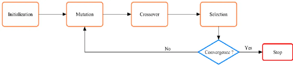
Differential Evolution (DE) is a stochastic optimization method which permits alternative solutions for some of the complex composite design and optimization problems such as increasing frequency and frequency separation and obtaining lightweight design. Differential Evolution algorithm includes the following main stages: initialization, mutation, crossover and selection as shown in Figure 4.1. The optimum results of the algorithm change with the parameters: scaling factor, crossover and population size. Detailed description of the DE can be found in Storn and Price (1997). Iteration process for the traditional numerical skims corresponds to a population in DE algorithms. It is relatively robust and efficient in finding global optimum of the objective function, but computationally expensive.

Figure 4.1: Flowchart of the DE algorithm. (Adapted from Vo-Duy et al., 2017) The first step of DE optimization process is initialization. There are several approaches to populate the initial generation. Random generation is widely used approach for solution. In this step, the algorithm maintains a population of r points, {x₁,x₂,…,x_k

,…,xr}, where typically r≫m, with m being the number of variables. Second step is “Mutation” and it is a genetic operator that maintains the genetic variety from one to another generation for the population. In mutation process, the solution can be different from the previous prediction, thus better solution is gained. In third step, “Crossover” is used to obtain a richer population. Genetic diversity is encouraged by the interchange of genetic material between chromosomes after that, the strings of corresponding chromosomes are split at the same solution and two parents create a child. Finally, “Selection” is applied and the new individual is added to the new population (Gurdal et al., 1999; Sivanandam & Deepa, 2008; Roque & Martins, 2015).

4.3.2 Simulated Annealing Algorithm

One of the most popular random search methods is SA. It mimics annealing phenomena that a metal object is warmed up to a high temperature and permit to cool slowly. The melting process lets the atomic structure of the material to pass to a lower energy condition, hence that becoming a tougher material. From the view point of optimization, in SA algorithm, annealing process lets the structure to get away from a local minimum, and to explore and settle on a better global optimum point. The main advantage of SA is that it enables to solve various optimization problems such as continuous, discrete or mixed-integer. In the working phase of this method, a new random point is produced for the iteration steps and as all stopping criteria are fulfilled the algorithm stops. Among the current point, the extension of the search can be produced by the probability distribution of Boltzmann.

/

( ) E kT

P E e (4.1)

where P(E) is the probability function of achieving the energy level E, k represents the Boltzmann’s constant, and T is temperature. In order to follow the procedure of the algorithm easily, the flowchart of a SA algorithm is presented in Figure 4.2.

Figure 4.2: Flowchart of the SA algorithm. (Adapted from Pham & Karaboga, 2000) Simulated Annealing algorithm has the following steps:

1. Start with an initial vector x₁ and assign a high temperature value to the function.

2. Generate a new design point randomly and find the difference between the previous and current function values.

3. Specify whether the new point is better than the current point.

4. If the value of randomly generated number is larger than eE kT/ , accept the point x_i1.

5. If the point x_i1 is rejected, then the algorithm produces a new design point

1

i

x_ randomly. However, it should be noted that the algorithm accepts a worse point based on an acceptance probability (Rao, 2009).

Table 4.1: DE and SA parameters used in optimization

4.3.3 Design Approach for Composite Materials

The design of the composite materials is a combined process including manufacturing properties, optimum fiber orientation angle of the composites and design of the structural components. Design goals are based on structural engineering application (see Table 4.2). Specific implementation requirements specify a combination of one or more fundamental design goals for:

 Stiffness

 Strength (fatigue and static)

 Dynamic and/or environmental stability  Damage tolerance (Daniel & Ishai 1994)

In the thesis study, stiffness is considered as design objective, and as a result, graphite fiber reinforced epoxy composite is selected as design material for high buckling load and small deflection.

Options Name DE SA CrossProbability 0.5 - RandomSeed 0 0 ScalingFactor 0.6 - SearchPoints - 1000 Tolerance 0.001 0.001 LevelIterations - 50 PerturbationScale - 1.0

Table 4.2: Design approach for composite materials (Source: Daniel & Ishai 1994)

CHAPTER 5

RESULTS AND DISCUSSION

5.1. Problem Definition

In this study, the stacking sequence designs of maximum critical buckling load factor are obtained for laminated composite plates considering different angle increments. Laminated plate is rectangular, simply supported on four edges with length of a and width of b and subjected to in-plane compressive loads N_x andN , as shown in y Figure 5.1. Detailed description of optimization problems are listed in Table 5.1. Furthermore, materials and their properties studied in this thesis are given in Table 5.2A, Table 5.2B and Table 5.2C in terms of different materials, Glass/Epoxy and Graphite/Epoxy, respectively.

Figure 5.1: Laminated composite subjected to in-plane loads (Source: Lopez et al., 2009)

Problem 1 is verification case so that 64 plies symmetric-balanced Graphite/Epoxy

composite laminated plate, is assembled of two-ply stacks (90 90) with 45

degree increments. Therefore, the number of design variables decreases from 64 to 16. The representation of stacking sequence of 64 layered composite plate can be given as

1 2 3 4 5 6 7 8 9 10 11 12 13 14 15 16

[ / / / / / / / / / / / / / / / ]_s Thickness of each layer is 0.25 mm, total thickness of the laminated plate t = 8.128 mm and the length of plate a equals to 0.508 m. Nx has been taken as 1000 N/mm

in the design process. N_y and b have been calculated from the load ratio (N /_x N_y) and the plate aspect ratio (a /b) accordingly. The critical buckling load factor (_cb) is used as an objective function in optimization. For each design, objective function is

got using Mathematica program. In order to obtain the critical buckling load factor_cb

, it is important to find the combinations of values m and n producing minimum

buckling load. If they are selected as 1 or 2 and unit loads are applied, the minimum of the pairs b

 

 

 





cb  .

In this study, the plate design has been studied under loading ratios;N_x /N _y 1,

/ 1 / 2

x y

N N  , N_x/N _y 2, and plate aspect ratios; a b / 2, a b / 1 / 2, a/b1.

Table 5.1. Optimization problems.

Firstly, fiber angles in the stacking sequences of the laminated composite materials have been assumed discrete under the interval (90  90) and the optimization has been implemented considering this assumption. Discrete ply orientations are utilized in the design of laminate composites because of the economical manufacture methods of the industry. It should be considered that the plies are noted as ± stacks for ensure the balance of the composite laminate. Moreover, the fiber orientation angles of the plate have been taken as design variables with 45 degree

increments during the optimization process. Load cases given in Table 5.3 are used for buckling load factor algorithm verification. Differential Evolution and Simulated Annealing are selected as two methods of optimization for the same problem in order to compare the solution of optimization problems given in Table 5.4 (Problem 1). Secondly, the problem 2 have been solved for different stacking sequences increments which are integer and discrete with 1-5-10-30-45 degree increments. Thus, the evaluation of the different degree increments is important in terms of price and ease of manufacturability. The effect of loading cases and angle increments on critical buckling load factor of laminated composites are shown in Table 5.5 and Figure 5.2 (Problem 2).

Thirdly, in order to investigate the effect of material types on critical buckling load factor, the optimization problems are solved for 13 different composites materials bsed on LC1 loading case and DE method. Table 5.7 and Tables 5.8A,B show comparison results about different materials in terms of critical buckling load factor (Problem 3).

Lastly, 10 different Glass/ Epoxy and 9 different Graphite/ Epoxy materials are used to see the effect of scattering of material properties on optimization results. The critical buckling load is calculated depending on the different material properties of Glass/ Epoxy and Graphite/ Epoxy given in the literature (see Table 5.9 and Table 5.10). In problem 4, DE method and LC1 loading cases are considered through the optimization process as similar to other case studies (Problem 4).

First of all, it is found that the critical buckling load factor values are close to those values given by (Karakaya & Soykasap, 2009) and (Deveci 2011). This means that, the present critical buckling load factor algorithm could yield reliable results given in Table 5.4. The critical buckling load factor values are close to each other but some results based on DE are better than the results by SA. LC3, LC6 and LC9 where the aspect ratios are ½, SA yields worse results than DE. In addition DE method find the results in much less timing. This shows that DE method is more effective for this problem. At the same time LC1, LC3, LC4, LC6 and LC9 have also been found to have different angles while the critical buckling value is not changing. On the other hand in LC2, LC5 and LC8 the buckling value and angle do not change where the aspect ratio is 1, even though the load ratio is changed. There are also the same angle arrays in the two optimizing methods. Also, as the aspect ratio decreases which are LC1-LC2-LC3, LC4-LC5-LC6 and LC7-LC8-LC9 and load ratio decreases that are

LC1-LC4-LC7, LC2-LC5-LC8 and LC3-LC6-LC9 the critical buckling value decreases.

The main purpose of problem 2 is to investigate the effect of the critical buckling load factor in terms of the angle increments. In Table 5.5, the results based on DE method for different (1, 5, 15, 30, 45) degree increments (corresponds to D1, D2, D3, D4, D5, respectively) are listed for the same problem. The results obtained by DE are calculated faster and more accurately than the results based on SA. Under LC2, LC5 and LC8 cases, the critical buckling load factor value calculated for 30 degree (D4) increment is 10% lower than the values calculated by other degree increments. In addition, in other angle increments, 0-7% variations are observed between the best and worst results. Therefore, it is sufficient to design using only 45 degree increment and it is also suitable for the manufacturing conditions (see also Figure 5.2 for better insight into the procedure).Variation of optimum stacking sequences with different increments are given in Table 5.6. It is obvious that for the loading cases LC2, LC5 and LC8 [ 45 ] 16 s are obtained except for D4.

The variation of the critical buckling load factors of widely used composite materials due to different degree increments is given in Table 5.7. The maximum critical buckling factor have been calculated using the DE method. Firstly, the critical buckling factor value deviations are at maximum 5% depending on the degree of increase. Therefore, when preferred the simplicity of production and the cost-effectiveness, it seems that D4, D5 angle increments are more suitable for use. Initially, it is observed that boron, graphite and glass epoxy have 2 to 3 times as high as the critical buckling value of the others. The critical buckling load factor of S-Glass Epoxy is about 16 times more than that of S-S-Glass Polyester while _cbof E-Glass Epoxy is about 1, 5 times more than that of E-E-Glass Polyester. As the most important natural fiber reinforced composites Flax / Epoxy and Flax / Polyester are compared it is seen that  of Flax / Epoxy is about 3 times higher than that of Flax / cb Polyester. In this context, the critical buckling load factor of materials with matrix epoxy is higher than that of matrix with polyester.

Table 5.8A-B describes the most preferred composite materials available in the literature for evaluation of buckling, depending on the plate loading conditions LC1