Analysis of spine sounds for spinal health assessment

ANALYSIS OF SPINE SOUNDS FOR SPINAL

HEALTH ASSESSMENT

a thesis submitted to

the graduate school of engineering and science

of bilkent university

in partial fulfillment of the requirements for

the degree of

master of science

in

electrical and electronics engineering

By

Mustafa Arda Ahi

May 2017

Analysis of Spine Sounds for Spinal Health Assessment By Mustafa Arda Ahi

May 2017

We certify that we have read this thesis and that in our opinion it is fully adequate, in scope and in quality, as a thesis for the degree of Master of Science.

Ahmet Enis C¸ etin(Advisor)

U˘gur G¨ud¨ukbay

H¨useyin Hacıhabibo˘glu

Approved for the Graduate School of Engineering and Science:

Ezhan Kara¸san

ABSTRACT

ANALYSIS OF SPINE SOUNDS FOR SPINAL HEALTH

ASSESSMENT

Mustafa Arda Ahi

M.S. in Electrical and Electronics Engineering Advisor: Ahmet Enis C¸ etin

May 2017

This thesis proposes a spinal health assessment system based on acoustic bio-signals. The aim of this study is to offer an alternative to the conventional spinal health assessment techniques such as MR, CT or x-ray scans. As conventional methods are time-consuming, expensive and harmful (radiation risk caused by medical scanning techniques), a cheap, fast and harmless method is proposed. It is observed that individuals with spinal health problems have unusual sounds. Using automatic speech recognition (ASR) algorithms, a diagnosis algorithm was developed for classifying joint sounds collected from the vertebrae of human sub-jects. First, feature parameters are extracted from spinal sounds. One of the most popular feature parameters used in speech recognition are Mel Frequency Cepstrum Coefficients (MFCC). MFCC parameters are classified using Artificial Neural Networks (ANN). In addition, the scattering transform cepstral coeffi-cients (STCC) algorithm is implemented as an alternative to the mel filterbank in MFCC. The correlation between the medical history of the subjects and the “click” sound in the collected sound data is the basis of the classification al-gorithm. In the light of collected data, it is observed that “click” sounds are detected in the individuals who have suffered low back pain (slipped disk) but not in healthy individuals. The identification of the “click” sound is carried out by using MFCC/STCC and ANN. The system has 92.2% success rate of detecting “click” sounds when MFCC based algorithm is used. The success rate is 83.5% when STCC feature extraction scheme is used.

Keywords: spinal sounds, sound analysis, sound and signal processing, wearable medical systems.

¨

OZET

OMURGA SESLER˙IN˙IN OMURGA SA ˘

GI ˘

GI

DE ˘

GERLEND˙IRMESI AMACIYLA ANAL˙IZ˙I

Mustafa Arda Ahi

Elektrik ve Elektronik M¨uhendisli˘gi, Y¨uksek Lisans Tez Danı¸smanı: Ahmet Enis C¸ etin

Mayıs 2017

Bu tez, eklem sa˘glık de˘gerlendirmesi i¸cin akustik biyo-sinyallere dayalı bir omurga sa˘glık de˘gerlendirme sistemi ¨onermektedir. Bu ¸calı¸smanın amacı MR, CT veya x-ray taramaları gibi geleneksel omurga sa˘glık de˘gerlendirme teknikler-ine bir alternatif sunmaktır. Geleneksel y¨ontemler zaman alıcı, pahalı ve zararlı (tıbbi tarama tekniklerinden kaynaklanan radyasyonun olu¸sturdu˘gu risk) oldu˘gundan bu ¸calı¸sma ile ucuz, hızlı ve zararsız bir y¨ontem ¨onerilmektedir. Omurga sa˘glık problemi olan bireylerde ola˘gan dı¸sı sesler tepit edilmi¸stir. Denek-lerin omurgasından toplanan eklem sesleri kullanılarak bir te¸shis algoritması geli¸stirilmi¸s, ¨oznitelik ¸cıkarımı ve sınıflandırmayı ger¸cekle¸stirmek i¸cin otomatik ses tanıma algoritmaları kullanılmı¸stır. ˙Ilk olarak, ¨oznitelik parametreleri omurga seslerinden ¸cıkarılmı¸stır. Konu¸sma tanıma i¸cin en pop¨uler ¨oznitelik ¸cıkarma y¨ontemlerinden biri olan Mel Frekans Kepstrum Katsayıları (MFCC) kul-lanımı¸stır. MFCC parametreleri Yapay Sinir A˘garı (ANN) sınıflandırma metodu ile sınıflandırılmı¸stır. Buna ek olarak, sa¸cılma d¨on¨u¸s¨um¨u cepstral katsayıları (STCC) algoritması, MFCC’deki mel filterbanka alternatif olarak uygulanmı¸stır. Deneklerin tıbbi ge¸cmi¸si ile toplanan ses verilerindeki ”klik” sesi arasındaki kore-lasyon, sınıflandırma algoritmasının temelini olu¸sturmaktadır. Toplanan veriler ı¸sı˘gında, bel a˘grısı (bel fıtı˘gı) ge¸ciren ancak sa˘glıklı bireylerde de˘gil, ’klik’ ses-lerinin algılanadı˘gı g¨ozlemlenmi¸stir. ’Klik’ sesinin tanımlanması MFCC / STCC ve ANN kullanılarak yapılır. Sistem, MFCC algoritması kullanıldı˘gında ’klik’ ses-leri tespit etmede %92.2 ba¸sarı oranına sahiptir. STCC ¨oznitelik ¸cıkarma ¸seması kullanıldı˘gında ba¸sarı oranı %83.5’dir.

Anahtar s¨ozc¨ukler : Omurga sesleri, ses analizi, ses ve sinyal i¸sleme, giyilebilir tıbbi sistemler.

Acknowledgement

I would like to dedicate my thesis to my mother who suffered spinal diseases for more than 15 years and currently live with a spinal platin implant. I would like to thank my whole family for their limitless support and encourage, especially to my beloved wife for editing my thesis.

I would like to express my sincere gratitude to:

• My thesis advisor Prof. Dr. Ahmet Enis C¸ etin for his patient and invaluable support for past four years.

• My thesis committee Prof. Dr. U˘gur G¨ud¨ukbay and Assoc. Prof. Dr. H¨useyin Hacıhabibo˘gu.

• Prof. Dr. Emre Acaro˘glu for medical consultancy.

• G¨okmen Can, Tolga Cerrah and Dr. Hakan T¨oreyin for their support and help.

Without their contributions, I would not have been able to accomplish completing this thesis.

Contents

1 Introduction 1

2 Background Information and Experiment 6

2.1 Related Work . . . 6

2.2 Data Acquisition Process . . . 8

2.3 Data Acquisition and Hardware Specification . . . 9

2.4 Mel-Frequency Cepstral Coefficients (MFCC) . . . 11

2.4.1 Pre Emphasis . . . 11

2.4.2 Framing . . . 12

2.4.3 Windowing . . . 12

2.4.4 Mel-Filter Bank . . . 13

2.4.5 Logarithm Operation . . . 17

2.4.6 Discrete Cosine Transform . . . 17

CONTENTS vii

3 Analysis of Spinal Sounds 18

3.1 Data Acquisition Method . . . 18

3.1.1 Data Acquisition Application . . . 18

3.1.2 Data Acquisition Environmental Conditions . . . 19

3.2 Data Analysis in Time Domain . . . 20

3.2.1 Data Pre-processing . . . 20

3.2.2 Time Domain “Click” Detection . . . 21

3.3 Mel Frequency Cepstrum Coefficients Feature Extraction Results . 27 3.4 Artificial Neural Network Classification Algorithm . . . 28

4 Feature Extraction With Scattering Transform 34 4.1 Scattering Transform Cepstral Coefficients Freature Extraction . . 34

4.2 STCC Feature Extraction Based on Uniform Filterbank . . . 35

4.3 STCC Feature Extraction Based on Non-Uniform Filterbank . . . 37

4.4 Detection Performance of Uniform and Non-Uniform Filterbank Based STCC . . . 38

5 Conclusion 40

List of Figures

1.1 Lower Lumbar Vertebrae . . . 1

1.2 Artificially Generated Recording . . . 5

2.1 Data Acquisition System . . . 10

2.2 MFCC Steps . . . 11

2.3 Framing and Windowing of Audio Signal . . . 12

2.4 Mel Scale vs. Frequency Scale . . . 14

2.5 Mel Scale Filterbank . . . 16

2.6 Mel Filterbank Energy Calculation [1] . . . 16

3.1 Android Application Graphical User Interface . . . 19

3.2 A section of Backbone Elements [2] . . . 20

3.3 Sound and Gyroscope Data of a Healthy Subject . . . 21

3.4 Possible “Click” Sound Data . . . 22

LIST OF FIGURES ix

3.6 Three Possible “Click” Sound Data . . . 24

3.7 Sound and gyroscope data of a different unhealthy subject . . . . 25

3.8 Three Possible “Click” dound data of a different unhealthy Subject 25 3.9 Power Spectrum Density of Average of “Click” Sound . . . 26

3.10 Mel Frequency Cepstral Coefficients of an Unhealthy Subject’s Data 27 3.11 Mel Frequency Cepstral Coefficients of an Unhealthy Subject’s Data 28 3.12 Mel Frequency Cepstral Coefficients of Healthy Subject’s Data . . 28

3.13 Two Layer Feed Forward Network . . . 29

3.14 Artificial Neural Network Data Distribution . . . 29

3.15 Confusion Matrix Output of ANN . . . 30

3.16 Probability of a “Click” Sound for Each Frame for Unhealthy Sound 32 3.17 Probability of a “Click” Sound for Each Frame for Healthy Sound 32 3.18 Confusion matrix of all subjects . . . 33

4.1 Block Diagram of STCC Feature Extraction . . . 35

4.2 Fourth order uniform filterbank with linear scattering . . . 36

4.3 Non-uniform filterbank with linear scattering . . . 37

4.4 Scattering Transform Cepstrum Coefficients . . . 38

LIST OF FIGURES x

A.2 Click Detection Probability of Unhealthy Subject 2 . . . 47

A.3 Click Detection Probability of Unhealthy Subject 3 . . . 47

A.4 Click Detection Probability of Unhealthy Subject 4 . . . 48

A.5 Click Detection Probability of Healthy Subject 1 . . . 48

A.6 Click Detection Probability of Healthy Subject 2 . . . 49

A.7 Click Detection Probability of Healthy Subject 3 . . . 49

List of Tables

2.1 Boya BY-M1 Omnidirectional Microphone Specifications . . . 9

3.1 Neural network classification true class detection success rate (%) of MFCC . . . 31

3.2 MFCC performance success rate (%) according to number of fil-terbank channel . . . 31

4.1 Neural network classification true class detection success rate (%) of uniform STCC . . . 38

4.2 Neural network classification true class detection success rate (%) of non-uniform STCC . . . 39

Chapter 1

Introduction

The spine is the row of connected bones from end of the head to the tail and it is responsible for preserving the nerves. It consists of 33 bones which are called the vertebrae and it is the basis of human skeletal system. The first 24 vertebrae are cushioned by small discs, some form of cartilage, and this provides spine the ability to bend and flexibility. The ruptured intervertebral disk symptom occurs in the lower part of the spine which is called the lumbar spine. As it can be seen in Figure 1.1, the lumbar spine consists of five vertebrae.

Figure 1.1: Lower Lumbar Vertebrae

Spinal health problems may occur because of infection, injury, tumor, degen-eration and aging factors and may cause the pain that may limit daily activities [3]. In Turkey between 50 to 80 percent of Turkish citizens experience some form

of back pain in their lifetime [4].

In the United States of America, an estimated 75 to 85 percent [5] of popu-lation suffers from back pain in their lifetime. Most of the time, the cause of the back pain is linked to the spine and in order to understand or diagnose a patient, a spinal health assessment is needed.

Spinal health assessment is achieved by using imaging techniques such as MR, CT, and/or X-ray in a clinic [6]. These methods can provide detailed infor-mation with respect to spinal degeneration and abrasion. However, they are time-consuming and cost ineffective.

In order to obtain medical images for a possible diagnosis, patients are making a sacrifice by being exposed to significant amounts of radiation. Moreover, results obtained from imaging techniques and the pain felt by patients generally do not correlate well and as a result patients are exposed significant amounts of radiation.

There is an alternative health assessment technique; namely spine sounds, which offers another opportunity to analyze spinal diseases by investigating the bio signals. Assessment of spine health with both acoustic and imaging tech-niques expands the information of diagnosis that has been gathered thus far. The structures that make up the spine produce sound during movement. Various characteristics of the backbone audio signals to be recorded with the microphones placed on the skin. Thus, the spinal sounds can be determined by signal process-ing algorithms. It is expected that the characteristics of the spine sounds will be influenced by changes in the spine structure. An ”acoustic signature” sound can be obtained for a healthy spine by producing sounds that are produced by a healthy spinal cord disk and are collected by microphones on the skin. If structural changes occur in the tissues of the spinal cord, the acoustic signature signals will change because of the injured tissues generate different sounds. By tracking the change of acoustic signature, spinal sound health assessment can be accomplished.

sport background, injuries and diseases. Data acquisition from pre-diagnosed patients helps to classify patients and allows to create an acoustic signature. Patients with pain or pre-diagnosed diseases generate different spinal sounds and the difference between acoustic signatures is the indicator of the problematic spine.

Data acquisition method is the key for a healthy classification process. The acquisition should simultaneously provide the movement and sound data and the process have to be quick, cheap, mobile and repeatable. Joint health assessment [7] study is a guide of the data acquisition and analysis processes. The data has been collected simultaneously by a gyroscope and a microphone and in time domain statistical data analysis has been made. When the subject bent his/her knee a joint sound was detected and this “click” sound was analyzed statistically.

Implementation of the same technique for spinal sounds is the solution of the data acquisition problem. In [8] the data acquisition and evaluation process has been given. Since both knee and spine bio signals are basically generated by bones, cartilage and muscles, we can analyze both signals in a similar fashion. Thanks to this resemblance, hardware equipment with similar specifications can be used in order to collect the spinal bio signals.

We offer a cheap, fast and reliable data acquisition process for the spinal sounds. An Android application helps us to use the sensors and microphone input of an Android smart phone. The first step of the thesis is developing an Android app that acquires data from sensor and microphone with a desired sampling rate. Since the built-in microphone of the smart phone does not have a good quality, an external microphone has been used. The Bio signal Data Acquisition System (BDAS) can collect the data anywhere, anytime and can acquire the data only in a few seconds. By using BDAS, data acquisition from healthy and unhealthy subjects has been completed and offline data analysis process has begun.

Although the human speech signal is non stationary, it is short-time stationary. By using this property, taking multiple short frames from speech data allows an

analysis for the data. In speech recognition, this analysis provides the acoustic sig-nature information for sounds that have been generated by the vocal track. This acoustic signature provides the information to apply automatic speaker recogni-tion (ASR) and classificarecogni-tion algorithms [9]. Consequently, ASR can be used for classification of the bio signals, which is called automatic bio signal recognition (ABR).

Feature extraction of bio signals is the most important part of the classifica-tion. This is because the process of feature extraction is unique for each subject. Therefore, for each subject, a different acoustic signature will be observed. In order to have robust classification, more conventional methods can be used, for instance a manual search for a “click”. In [8] “click” sound definition has been given and by searching this pattern in unhealthy subject’s data, a feature for spinal disease can be found and confirmed with ABR. The block diagram of the ABR system is given in Figure 1.2.

This thesis continues with the analysis of feature vectors by using the Mel Frequency Cepstral Coefficients (MFCC). The MFCC is widely used in speech recognition systems and it enables the unique opportunity of frequency analysis in a series of consecutive time frames. As a result, we can analyze the frequency components of the complete sound signal which is divided into frames [10]. An alternative feature detection algorithm called Scattering Transform Cepstral Coefficient (STCC) is used to increase the classification performance of the MFCC algorithm.

For a complete ABR, a pattern recognition neural network is implemented in Matlab’s Neural Pattern Recognition Application. Input of pattern recognition are cepstrum coefficients which are MFCC coefficients in each frame. In order to train the neural network, previously (manually) detected “click” locations are used. Corresponding “click” location is transformed into MFCC matrix frame number and the MFCC coefficients in the frame is the basis of classification. All sampled sound signals are divided into two classes which are defective and healthy. “Click” locations are marked as defective and all other locations represent the healthy class.

Figure 1.2: Artificially Generated Recording

After training of neural network, in the light of the pattern recognition training of the neural network, ABR algorithm is synthesized. The input of the algorithm is the spinal sound signal and the output is the classification of the sound signal in each frame. If a “click” sound is detected, ABR detects it and indicates the location of the “click”. Subsequently, we have developed a system which acquires sound and gyroscope signals and detects the “click” sound when spinal movement occurs.The description of “click” sound is based on the data of patients who had undergone surgery and had been previously diagnosed. Since the “click” sound refers ruptured intervertebral disk syndrome, other disorders and diseases may not reveal in our method.

Chapter 2

Background Information and

Experiment

In this chapter, we present

• related work,

• data acquisition process,

• data acquisition hardware specification, and

• Mel Frequency Cepstrum Coefficients algorithm.

2.1

Related Work

To the best of our knowledge, spinal sounds had never been used for the spinal health assessment. On the other hand, over the past 40 years,studies have been carried out to evaluate the sound of the joints (i.e., knee, wrist, shoulder) in terms of joint health assessment [11].

This thesis, which studies the spine sounds for the first time, benefits from the experience gained from the studies on the sounds of the movable joints. Therefore, we represent a detailed summary of related works.

A great majority of joint sound studies were carried out with the aim of iden-tifying a variety of joint disorders and classifying the sound of numerous joint sounds collected from healthy subjects and persons with diseases according to various characteristics. These studies were conducted in three main research groups. The first of these, University of Akron Group, acquired the joint sounds from an airborne microphone which is located off the skin and by using a dif-ferent microphone, they acquired the background noise sound. From acquired joint sound and background noise sound, they accomplished to differentiate the healthy and unhealthy joint sounds with calculating the power of the joint sounds [12]. The second group, Queens University, reduced the problem of background noise by collecting joint sounds with vibro-meter receivers in contact with the skin instead of airborne microphones.This group has shown that every new mea-surement of many variables (such as skin surface friction or joint motion velocity) during sound measurements can lead to large differences in signal strengths (sig-nal intensity, click sound density, etc.), even if they are made from the same joint of the same person [13]. The last group, the University of Calgary, classified knee joint sound data from 90 people with artificial neural networks to a variety of properties (e.g., skewness/kurtois of probability density function) in the time and frequency domain [14], [15], [16].

In these studies it has been shown that the classification of joint disturbance can be performed with high accuracy [16]. These studies have provided the basis for the field of joint sounds and presented the results in this field with many hopes and promises. Today, joint sounds are evaluated in terms of joint health assessment; despite its great advantages of being non-invasive and harmless, it is far from being perceived as a clinical acceptable bio-signal.

In this thesis, in the light of previous joint sound related works, we form a basis of spinal health assessment analysis in order to bring joint sounds closer to clinical acceptance with a cheap and fast method.

2.2

Data Acquisition Process

In order to develop a universal signal processing algorithm that can determine joint disease and severity, it is necessary to precisely classify the population of patients and healthy individuals whom the sound data is to be collected, and the inclusion criteria must be carefully determined. For that reason we used pre-diagnosed patients for unhealthy subject set. For unhealthy subject test, only ruptured intervertebral disk syndrome diagnosed patients are accepted. This criteria allowed us to analyze the problem in a more specific manner with a selected disease classification.

One of the most important points to note when collecting data is the necessity of keeping the reproducibility of the data collection method high. Thanks to the cheap and easy repetitive method, measurement errors can be avoided and various sources of noise can be kept under control.

As it is not known the frequency and bandwidth of the bio-signal, it is necessary to have a high bandwidth (approximately 20 kHz) with low loss and low noise specified microphone. It is important that these enhancements are compact, lightweight, have low power consumption and wearable due to generate a large number of data set with the aim of producing a personalized joint sound model.

In the literature research, statistical inferences were made from the whole of the record after the noise of the joints sound recordings were suppressed by various filters. In this way, some of the studies based on the holistic approach have yielded high success rates in the distinction between unhealthy joints and healthy joints, but a universal algorithm that can achieve high success [16] in all databases has not been developed [11].

On the other hand, structural distortions occurring in the joints can be deter-mined not only by looking at the whole of the produced sounds but by examining only certain characteristic qualities specially. Therefore, in the analysis of sound recordings, as an alternative to the holistic approach in the literature, it may be necessary to classify the sound qualities with high resolution and separately

monitor the changes in the qualities of the sound signals belonging to each class.

In this thesis, the spine sounds examined for the first time and differently from previous knee joint sound studies. Thus, this thesis is envisaged to increase the sharpness of the information obtained from the spinal sounds.

In previous studies, the qualities examined to distinguish whether the joint is healthy or sick and to detect the severity of the disease are either obtained from the whole of each of the collected sound recordings (such as the total power of the signal) or by a single criterion (such as a certain frequency interval) and correlations of these qualities were examined with medical imaging results. On the other hand, in order to analyze the potential clinical value of the spinal sounds, acquired information compared with patient pain level and medical background.

2.3

Data Acquisition and Hardware

Specifica-tion

Earlier, joint sounds were not recorded with a wearable system. In other words, the systems in the literature are not designed to make joint health assessments in a quick and cheap method without the necessity of hospital environment. In order to develop a cheap, quick and feasible data acquisition method, we used smart phones because it is portable and almost every person has a smart phone. We developed an Android application which records microphone and internal gyroscope data. As the quality of the sound data is the key element of the data acquisition process, we used an external microphone with desired bandwidth, signal to noise ratio (SNR) and sensitivity given in the Table 2.1.

Table 2.1: Boya BY-M1 Omnidirectional Microphone Specifications Frequency Range 65Hz-18KHz

Signal/Noise 74dB

Sensitivity -30dB+/-3dB/0dB=1V/Pa,1kHz Transducer Electret Condenser

To record the data, subjects need to plug the microphone into the microphone jack of their smart phone and attach the microphone to their back with kinesio tapes. Those tapes are used for medical treatment by athletes but we preferred them because of their elastic property which induce less noise in a possible friction. Since we record spinal sounds with an airborne microphone, we need a very silent place to record the sound data. After microphone insertion; subject stands up, holds the smart phone, starts the application and leans forward until their torso is perpendicular to the legs and slowly stands up again. After several stand up-lean repetition, subject stops the recording see Figure 2.1.

Figure 2.1: Data Acquisition System

The Android application records the sound data with 44.1 kHz sampling rate and records gyroscope data with 1 kHz sampling rate. Gyroscope sensor acquires data while the subject holds the smart phone and by using this data we can simul-taneously correlate movement and sound data. Thus, it is possible to indentify click sounds by using gyroscope data. For instance, if all clicks are identified while the subject is in the same position then we can accept the corresponding click as a valid signal.

2.4

Mel-Frequency Cepstral Coefficients (MFCC)

The shape of the vocal track and the position of the tongue and teeth generates sounds, and from these sounds phonemes and from phonemes words are created. If the shape of vocal instruments are determined correctly, we can estimate the words or phonemes. This estimation problem is the basic description and moti-vation of automatic sound recognition (ASR) process and it is called as feature extraction. The MFCC is one of the most popular technique for ASR. The shape of previously mentioned vocal instruments determines the envelope of the short time power spectrum. MFCCs are series of vectors which represents envelope power spectrum of short sound frames. The implementation steps of the MFCC is given in Figure 3.10.

Figure 2.2: MFCC Steps

2.4.1

Pre Emphasis

The equation of the pre-emphasis block is defined in Equation 2.1.

y[n] = x[n] − 0.95x[n − 1] (2.1)

The purpose of the pre-emphasis process is to reduce the energy of the signal at lower frequencies. This is applied because high frequency components of the audio signal have less power than lower frequency components. In the acquired

data, noise signal has higher amplitude at lower frequencies thus we can apply this process to our customized MFCC [17], [18].

2.4.2

Framing

Since audio signals are constantly changing, we analyze them in short periods in time domain. In short time scale the audio signal does not change much, in other words it is statistically stationary. To analyze audio signal in short duration of time, we divide the signal into frames which is illustrated in Figure 2.3.

Figure 2.3: Framing and Windowing of Audio Signal

The frame width is typically 25ms with 10ms overlap. In this scenario, frames are 15ms shifted but it is statistically stationary. If we chose a greater frame width, the correlation between two consecutive frames will increase and this will result non-stationary process.

2.4.3

Windowing

The computation of DFT based on an assumption of continuity. In other words,the first point and the last point of the input signal must correlate highly and form a continuity [19]. If there is discontinuity in the input frame, undesired artifacts occur in spectrum after DFT operation.

w[n] =    0.54 − 0.46 cos(_{N −1}2πn), if n ≥ N 0, otherwise (2.2)

We multiply each frame with a smoothing function which smoothly attenuate both ends of the signal due to prevent this phenomena. For this purpose, we used hamming window as its spectrum attenuates faster than other windows.

2.4.4

Mel-Filter Bank

2.4.4.1 Mel Scale

Human ear is not equally sensitive to all frequency bands. We can hear lower fre-quencies better than higher frefre-quencies. As a result human ear is more sensitive to small variations in low frequency band.Mel is a unit of pitch and pitch dis-crimination is better at low frequencies while higher frequencies have worse pitch ratio [1]. Mel scale is roughly linear up to 1KHz and after 1KHz it is roughly logarithmic. To illustrate, human ear is a series of band-pass filters which has a non-linear distribution for an approximation of the mel scale compared to linear scale see Figure 2.4.

We can transform the linear-scale to mel-scale in frequency domain with Equa-tion 2.3 M el(f ) = 2595 × log₁₀(1 + f 700) (2.3) or with Equation 2.4 M el(f ) = 1125 × ln (1 + f 700) (2.4)

Figure 2.4: Mel Scale vs. Frequency Scale

2.5 [1]

M el−1(m) = 700 × e1125m −1. (2.5)

2.4.4.2 Mel Filterbank Implementation

Mel filterbank is one of the most important steps in the MFCC implementation. We convert linear-scale to mel-scale and use this scale in order to determine the center frequencies of series of band-pass filters. We use filterbank to create a series of band-pass filter. Filterbank is an array of band-pass filters which allows us to analyze the signal in divided sub-segments in frequency domain. This analysis method is called as wavelet analysis and is very useful for analyzing the signal in frequency domain.

Mel filterbank is implemented in five steps:

• According to sampling frequency, we determine the upper and lower fre-quencies and converts the limits to mels. Use Equation 2.3.

• We Determine the number of filters in filterbank. For n filterbank, there are n+2 frequency values. These values are spaced linearly in mels. For that reason, we have divided the mel-converted frequency values into equally spaced segments in the limits of calculated upper and lower frequency values which were converted into mels.

• By using Equation 2.5, convert the mel-scaled array into linear-scale. Notice that, the equally spaced array in mel-scale is not equally spaced in linear-scale, yet our start and end points in first item are conserved and mel-scaled spaced.

• By using FFT, we have limited resolution in frequency domain. For that reason we have to round the calculated mel-scale array in order to fit them on the nearest FFT bin. To determine the FFT size and by using sample rate information we use Equation 2.6. Where N is fft order and fs is sample rate.

f (i) = f loor((N + 1) × h(i) fs

) (2.6)

• Create filterbanks. First filter starts on the first point and reaches its peak on the second point than return to 0 at third point. Second filter starts at second point and reaches its peak on the third point than return to 0 at fourth point and so on. By using Equation 2.7 we can calculate the amplitude of the filter according to filter number m and frequency f() [20].

Hm(k) =                0, if k < f (m − 1) k−f (m−1) f (m)−f (m−1), if f (m − 1) ≤ k ≤ f (m) f (m+1)−k f (m+1)−f (m), if f (m) ≤ k ≤ f (m + 1) 0, if f (m − 1) ≤ k ≤ f (m) (2.7)

In Figure 2.5, filterbanks are uniformly distributed in mel-scale with proper start and end point.

Since filters in Figure 2.5 have different frequency widths, filters do not have equal gain distribution. Nevertheless it is experimentally observed that in speech recognition there is no need for such application [19].

Figure 2.5: Mel Scale Filterbank

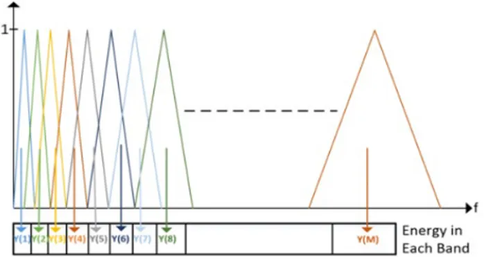
After mel-scaled filterbank implementation, we apply it to the spectrum of the signal. After this step, we calculate the energy of the output signal in for each filterbank. Multiplication of filterbank triangle and signal magnitude inside the filterbank in frequency domain and adding up the coefficients results the output energy for a filterbank. This application is visualized in Figure 2.6.

Figure 2.6: Mel Filterbank Energy Calculation [1]

At the end of this step, we acquired an array of Y(m), which consists of energy in each filterbank.

2.4.5

Logarithm Operation

Logarithm operation compress the dynamic range of values. Human ear has logarithmic response, namely, it is much sensitive to low amplitude sounds rather than higher amplitudes. To this end, the logarithm Y(m) is computed. Thanks to this step, slight variations in Y(m) will not effect the output.

2.4.6

Discrete Cosine Transform

Taking the Discrete Cosine Transform (DCT) of the logarithm of mel-spectrum converts it into another domain via Equation 2.8. The output result is a single Mel Frequency Cepstral Coefficient (MFCC) [1].

y[k] = M X m=1 log(|Y (m)|) cos (k(m − 0.5)π m ), k=0, 1, ..., M-1 (2.8)

2.4.7

Deriving MFCCs

After DCT, a single vector MFCC was gathered. If we respectively apply mel-filterbank, logarithm and DCT operation to all frames, we will create a series of MFCC vectors for a given sound signal. Thus, a matrix of the MFCCs is generated. For each frame, an array of coefficients created and we can analyze the joint sound signals in time and frequency. Thanks to this powerful feature extraction technique, we can analyze the data in both time and frequency domain and we can detect in which frame the frequency of the click sound present.

Chapter 3

Analysis of Spinal Sounds

In this chapter, we present

• data acquisiton method,

• data analysis in time domain, and

• mel frequency cepstrum coefficients feature extraction results.

3.1

Data Acquisition Method

3.1.1

Data Acquisition Application

Data acquisition methods are one of the most important steps in this thesis. Since there are not referable studies and data sets available for cross check, we have to make sure the validity of the experiment data. To ensure that, we have developed an Android application that records the sound data with 44.1KHz sampling rate and the gyroscope data with 1KHz sampling rate. We have tested our application in order not to encounter with possible data discontinuity and incoherence be-tween the sound and gyroscope data. Even though we don’t have the information

of spinal sound (either unhealthy or healthy), we take the reference of [21], [8] in order to detect/identify the “click” sound.

In the light of previous knowledge of “click” sounds and their previously ob-served possible occurrences according to the position of the joint, we prefer to start analysis in time domain with the help of coherently acquired gyroscope data. Hence the coherency of the gyroscope and sound data is crucial. As it can be seen in Figure 3.1, Android application graphical user interface is simple and easy to use.

Figure 3.1: Android Application Graphical User Interface

3.1.2

Data Acquisition Environmental Conditions

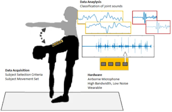
Spinal sounds from 24 individuals were recorded. Of these, 12 were unhealthy and 12 were healthy individuals. Three of the patients had a surgery and 5 patients had MRI results that proved their discomfort. Having acquired the sound data with the help of a microphone, we had to avoid the background noise. In order to minimize the noise in the sound data, data acquisition environment had to be completely quite. We attached microphone to subject’s waist with Kinesio elastic plasters while subject was holding the mobile phone. The test movement that subject had to repeat was bending to reach the feets and then standing upright. This exercise causes the movement of spinal column and it is similar with the bending knee movement in [7]. This exercise continuously increases and decreases the stress on the disks and cartilage tissue, Figure 3.2, and we listen their reaction to this movement.

Figure 3.2: A section of Backbone Elements [2]

3.2

Data Analysis in Time Domain

In order to detect and identify the “click” sounds, we started data analysis in time domain. By using the waveform information of the “click” sounds, we aimed to detect the “click” sounds in our data set. Amplitude of the “click” and occurrence of it, related to the position of the patient, determines the distinction between healthy and unhealthy spinal sounds.

3.2.1

Data Pre-processing

To analyze the data in time domain, various pre-processing steps are required. Gyroscope data is given in angular velocity form and in order to use gyroscope data, instead of angular velocity, angle value is required. For that reason a simple integration of gyroscope data was accomplished. In order to remove the undesired background noise, sound data was filtered by a band-pass filter.

3.2.2

Time Domain “Click” Detection

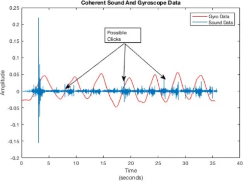
In the light of the knowledge of the shape and duration of a “click” sound [8], it is possible to seek similar waveform in acquired data set. In Figure 3.3, sound and gyroscope data gathered from healthy subject plotted together. It is possible to correlate the subjects’ movement with possible “click” sound. Gyroscope data, identified with red color, represents the angle of the subject. Initial position is stand tall (180◦) which is negative peak and last position of the subject is approximately 90◦ bending position. As it can be seen while subject covers a region of 90◦, angle value gathered from gyroscope behaves similar to a sinusoidal signal.

Figure 3.3: Sound and Gyroscope Data of a Healthy Subject

Sound data in Figure 3.3 has various strong and minor peaks. The amplitude of the gyroscope data was normalised according to sound signal. The strongest peak is a possible noise sound caused by the microphone contact with the skin. Minor peaks are possible “click” sounds yet they have to be examined separately. In order to identify a short time period as a “click” the waveform must satisfy following conditions; location of the “click” sound have to be periodic with angle

value, shape/duration of the signal have to be periodic with angle value and shape/duration of the signal have to be similar with the known “click” sound [8] also as we listen the data, a “click” sound can be heard.

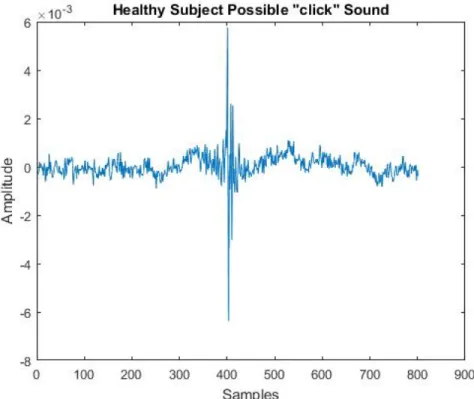
Figure 3.4: Possible “Click” Sound Data

In Figure 3.4, a possible peak signal was observed and neither the shape of the signal nor the duration was similar with the “click” sound. Duration is approximately 0.5 ms, which is much less than 2-3 ms — duration of a “click” sound.

After a careful analysis in time domain, neither a valid “click” sound nor desired periodicity in possible peak locations were detected. We searched peaks of the sound signal search for possible “clicks”. In the analysis of all signals in healthy subjects’ data set, we could not detect a valid “click” sound.

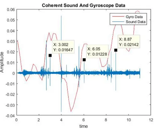
A combination of sound and gyroscope data of an unhealthy (slipped disk) subject is given in Figure 3.5. The possible “click” locations are marked. The importance of the possible “click” locations is that they are located at local

Figure 3.5: Sound and Gyroscope Data of an unhealthy Subject

extrema locations of the gyroscope data.

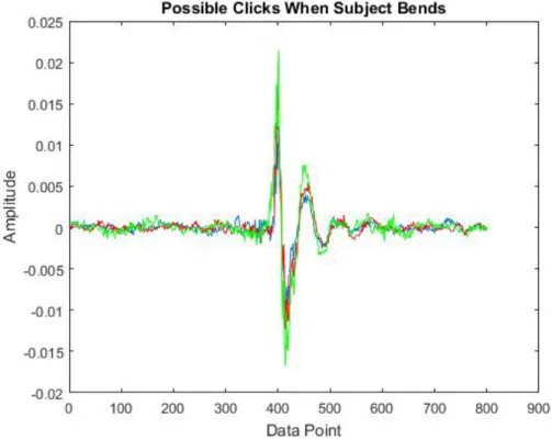
In Figure 3.6 possible “click” sounds were plotted with aligned starting point. Three signal perfectly align with each other and duration of the signal is approx-imately 3.5 ms (since the sampling rate is 44.1KHz, 150 point contains “click” data). Periodicity and the consistency properties of the possible “click” sounds confirm that the detected signal is a “click” sound with high probability.

Since the observed possible “click” sound also exists in other measurements in unhealthy subjects’ data set, we can reach the conclusion that the “click” sound is a valid indication of an unhealthy spine sound.

In Figure 3.7, possible “click” locations in another subject’s data are given. Similar to Figure 3.5, Figure 3.7 has the potential “click” locations when gyro-scope data reaches its maximum angle value, the subject bends and the angle between torso and legs is approximately 90 degree.

Figure 3.6: Three Possible “Click” Sound Data

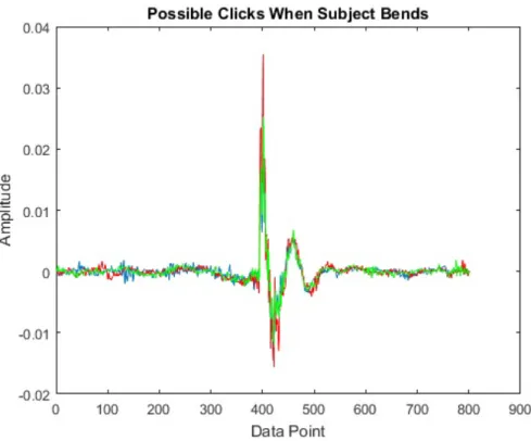
The shape and the duration of “click” signal from another data of unhealthy subject data-set (see Figure 3.8) is very similar with previously detected pattern. Moreover, the locations of the detected “click” signal shares the same pattern in all unhealthy subjects. By contrast, healthy subjects’ data set does not contain a valid “click” signal. Therefore, a pattern recognition technique is implemented by the assumption that the data with the “click” sound belongs to unhealthy individuals.

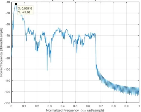
It is also observed that the Power Spectrum Density (PSD) of the “click” sounds has approximately 2KHz bandwidth (see Figure 3.9). As a result, we have acquired the frequency and time information of a “click” sound.

Figure 3.7: Sound and gyroscope data of a different unhealthy subject

3.3

Mel Frequency Cepstrum Coefficients

Fea-ture Extraction Results

In order to identify a “click” sound in a continuous sound record, MFCC feature extraction method is used. By dividing the signal into many short duration frames, it is possible to analyze the signal in both time and frequency domain. The MFCC frame duration is 25ms with 10ms time shift and “click” sound duration is 5ms, thus it is possible to cover a “click” duration in two frames but with an overlap. Therefore this may result in a false alarm or misdetection. We use 40 filterbank channels where DCT order of the (number of cepstral coefficients) is 13.

Figure 3.10: Mel Frequency Cepstral Coefficients of an Unhealthy Subject’s Data

In Figure 3.10, the MFFC matrix of the data in Figure 3.5 is given. The “click” locations in Figure 3.5 are detected and referring frame indices are calculated and labeled. These labeled frames contains the MFCCs of detected “click” sounds. Furthermore, the first MFCC coefficients of labeled frames are significantly dif-ferent form the other frames. This is because the “click” information, which is at 700Hz, located inside of the first filterbank triangle. Labeled frames can be observed with lighter color in the first cepstral coefficient.

In order to analyze cepstrum coefficients in more detail, the plot for 4 cepstral coefficients is given in Figure 3.11. In Figure 3.12, a healthy subjects cepstrum coefficients are given. Differently, the first cepstral coefficient amplitude values are similar to each other in healthy subject’s cepstrum coefficients.

Figure 3.11: Mel Frequency Cepstral Coefficients of an Unhealthy Subject’s Data

Figure 3.12: Mel Frequency Cepstral Coefficients of Healthy Subject’s Data

In the light of what has been done thus far, a “click” sound feature was man-ually detected by using the MFCC feature extraction method. For automatic “click” detection, a classification algorithm is needed.

3.4

Artificial Neural Network Classification

Al-gorithm

In order to classify feature vectors, Matlab’s Neural Network Toolbox is used. Neural Pattern Recognition Application classifies features into two sets of target categories by using a two layered feed-forward network. Neural network structure

consists of two layers, hidden layer and output layer (see Figure ??). In our model we have 10 hidden layers.

Figure 3.13: Two Layer Feed Forward Network

Neural pattern recognition app requires two input. First one is the data to be classified; in our case it is the MFCC feature matrix which is thirteen-by-N matrix. Second input is the class identifier. In our case we have two classes, healthy and unhealthy. Therefore, we created a two-by-N identifier matrix where N is the number frames in the MFCC feature matrix and is equal to 1120. If a frame is known to contain these “click” feature, the first row of the class identifier matrix is ’1’ in related frame number. Otherwise second row of identifier matrix is ’1’.

Figure 3.14: Artificial Neural Network Data Distribution

As a result, we classified the given MFCC matrix and feed it to the application for training process. Thanks to the training process, application updates the weights according to the scaled backpropagation method [22].

The MFCC feature matrix contains 1120 frames, which means there are 1120 samples for neural network application. As it can be seen in Figure 3.14, ran-domly chosen 70% samples are used for training, 15% for validation and 15% for

testing. Since testing, validation and testing data have been chosen randomly, the performance changes in every iteration.

Figure 3.15: Confusion Matrix Output of ANN

In order to measure the performance of the artificial neural network, a con-fusion matrix is used. The concon-fusion matrix indicates how many class elements exist in each step (training, validation and testing). For a single iteration, the success rate for finding “click” feature of the classification algorithm is95.7%. In Figure 3.15, the confusion matrix for classification algorithm is provided where class 1 represents “click” sounds and class 2 represents environment noise. We have 26 frames that contain “click” sounds and 1094 frames contain environment noise. As it can be seen, 22 out of 26 “click” sounds are detected with 95.7% true class success rate (input class is 1 and output is also 1). Since the success rate

changes with the randomly chosen training data set, an average success rate is needed to measure the performance.

MFCC classification performance analysis is completed with 25 ms frame du-ration, 10ms frame shift and 300Hz-2700Hz filterbank frequency interval. In Table 3.1, performance analysis of the MFCC classification algorithm with 40 filterbank channels (M) according to the change of cepstral coefficients (C) is given. The performance analysis of MFCC classification algorithm with respect to number of filterbank channels is given in Table 3.2.

Table 3.1: Neural network classification true class detection success rate (%) of MFCC C Train 1 2 3 4 5 6 7 8 9 10 Mean 13 94.1 94.7 72.0 90.0 90.0 88.9 94.7 85.7 85.0 81.0 87.6 16 94.4 100 94.7 85.7 92.9 86.7 94.4 81.8 100 91.7 92.2 20 94.4 90.0 93.8 94.7 90.0 72.0 89.5 90.0 89.5 94.7 89.8

Table 3.2: MFCC performance success rate (%) according to number of filterbank channel

Cepstral Coeff C M=10 M=20 M=40

13

88.9

85.6

87.6

16

90.4

90.6

92.2

20

87.3

84.9

89.8

After the training process, the application produced a script that classifies the input MFCC matrix in light of previously given MFCC-Classifier matrix training. The output vector is the probability of a“click” sound for each frame in the given MFCC matrix. An unhealthy subject’s data is given to the Automatic Click Recognition(ACR) algorithm and output vector is given Figure 3.16.

Matlab’s ANN tool produces a classifier method after training process. The output the classifier is the propabilites of each frame between 0 and 1. If the

Figure 3.16: Probability of a “Click” Sound for Each Frame for Unhealthy Sound

value is closer to the 1, the detected signal is a click sound otherwise classifier output is closer to 0. In order to avoid false alarms, a threshold value, which is set to 0.6, is needed to detect the “click” sounds. If probability of a click sound is greater than 0.6 out of 1, we can say that a “click” sound exist. For instance, in Figure 3.17, a healthy data is given to the ACR algorithm and there is not a single frame probability that exceeds the threshold value. On the other hand unhealthy subject’s data exceeds threshold for five times. Other examples are shown in Appendix A.

Figure 3.18: Confusion matrix of all subjects

The confusion matrix for all 24 subjects is given in Figure 3.18. After the application of the classification algorithm, all classes identified successfully for both healthy and unhealthy subjects. When there is a “click” sound the ANN produce possibility values of above 0.6. If the “click” proability is above of the determined threshold, 0.6 out of 1, the data in the frame contains “click” sound. Based on this threshold it is possible to classify all the healthy and unhealthy subjects. None of the healthy subjects can have more than 0.6 value.

Chapter 4

Feature Extraction With

Scattering Transform

Scattering transform is proposed as an alternative method for feature extraction. Similar to MFCC, wavelet analysis of the data is handled with scattering trans-form. Discrete wavelet transform (DWT) coefficients are ”scattered’ by adding non-linearity in each step of filterbank [23] [24]. A custom filterbank is used instead of mel-filterbank as discussed in Chapter-2.

4.1

Scattering Transform Cepstral Coefficients

Freature Extraction

Similar to MFCC feature extraction method, scattering transfrom cepstral co-efficient (STCC) based feature extraction contains pre-emphasis, framing, win-dowing, logarithm and DCT blocks. The major difference between STCC and MFCC is filterbank block. In STCC instead of mel-filterbank, scattering trans-form is used to implement filterbank. The block diagram of STCC is given in Figure 4.1.

Figure 4.1: Block Diagram of STCC Feature Extraction

Wavelet analysis is powerful for sub-band frequency analysis. Thanks to wavelet analysis, the frequency domain is divided into multiple segments in or-der to analyze the signal in desired frequency band. The kernel of a uniform filterbank is, a half band low pass filter and a half band high pass filter with dec-imation by two operation and the output result is two seperate signal where high pass branch contains high frequency components and low pass branch contains low frequency components [25]. Cascade connection of these kernels results a uniformly divided frequency band channels. The number of frequency sub-bands are equal to the number of cascaded kernels. In order to create a non-uniform filterbank, some branches are terminated during cascade filtering which results non-symmetric division of frequency band. Moreover, it has been shown that scattering operator increases the classification performance [26], [27]. We use, both uniform and non-uniform filterbanks for STCC based feature extraction.

4.2

STCC Feature Extraction Based on

Uni-form Filterbank

The uniform filterbank with linear scattering is given in Figure 4.2. In each step, high pass filter is described as g[n] and low pass filter is described as h[n]. To implement the filterbank, Matlab Wavelet Toolbox (wfilt function) is used.

We used the following Biorthogonal 5.5 filter pair:

h[n]={0 0 0.039 0.007 -0.054 0.345 0.736 0.345 -0.054 0.007 0.0039 0 0}

and

g[n] = {−0.013 −0.002 0.136 −0.093 −0.476 0.899 −0.476 −0.093 0.136 −0.002 −0.013} (4.1)

4.3

STCC Feature Extraction Based on

Non-Uniform Filterbank

Non-uniform filterbank with linear scattering is given in Figure 4.3. Because the click sound located at the lesser frequency of the spectrum, a filterbank de-sign that is dense at lower frequencies and sparse at higher frequency is created. Therefore, similar to mel-filterbank, the energy of each cepstrum consists of lower frequency filterbanks.

Figure 4.3: Non-uniform filterbank with linear scattering

Figure 4.4 gives the cepstrum coefficients of the train data set. Similar to MFCC, the click locations at the first coefficients contain higher energy than the others. However, the energy difference is considerably lower compared to the MFCC. Therefore, the ANN performance of the STCC is worse than that of MFCC.

Figure 4.4: Scattering Transform Cepstrum Coefficients

4.4

Detection Performance of Uniform and

Non-Uniform Filterbank Based STCC

Click detection performances are analyzed to compare STCC and MFCC. In Table 4.1, STCC with uniform filterbank performance results are given. Com-pared to MFCC, STCC with uniform filterbank implementation performs worse. Performance analysis is performed with fourth order uniform filterbank where frequency domain is divided into 16 identical regions. As a result, a single branch of filterbank has 2756Hz bandwidth in frequency domain.

Table 4.1: Neural network classification true class detection success rate (%) of uniform STCC C Trial 1 2 3 4 5 6 7 8 9 10 Mean 10 81.0 78.3 76.9 63.3 63.3 80.0 88.9 71.4 78.9 71.4 75.3 13 82.1 78.9 81.0 63.3 71.4 71.4 80.0 69.7 76.9 60.7 73.4 16 76.9 78.9 71.4 80.0 82.6 83.3 87.5 71.4 81.0 76.0 78.9

In Table 4.2 performance results of STCC with non-uniform filterbank are given. The main difference is that lower frequencies of the spectrum is denser compared to higher frequencies. Therefore, between 0-11024Hz the spectrum is divided into 8 identical regions where each has 1378Hz bandwith. Thus, non-uniform STCC performed better compared to unfiorm STCC.

Table 4.2: Neural network classification true class detection success rate (%) of non-uniform STCC C Trial 1 2 3 4 5 6 7 8 9 10 Mean 10 90.5 75.0 83.3 87.5 83.3 82.6 80.0 82.6 78.9 89.3 83.3 13 71.4 88.9 81.8 91.7 81.8 71.4 88.9 63.3 76.9 90.5 80.6 16 95.2 94.4 63.3 78.9 83.3 91.7 78.9 81.8 85.7 81.8 83.5

Chapter 5

Conclusion

In this study, acoustic spinal health assessment and classification algorithms are proposed. Joint sounds, which were generated from spinal movement, are col-lected for both healthy and unhealthy subjects. Acquired data analysis is ac-complished in both time and frequency domain. First of all, a “click” sound pattern is searched in both unhelathy and healthy subjects’ data. Coherent gy-roscope and sound data pair are used to determine the position of the subject in order to correlate the “click” sound with the position of the subject. As a result, “click” sound pattern is detected only in unhelathy subjects’ data set. Therefore, detection of the “click” sound is correlated with the unhealthy spinal cord.

Secondly, feature extraction algorithms for speech recognition are used. MFCC method is widely used in Automatic Speech Recognition systems to extract fea-tures in speech data. By using MFCC method, joint sound recordings are ana-lyzed in both time and frequency domain. In this thesis, we used MFCC feature extraction to divide the sound recordings into short frames, analyze the data in frequency domain and determine a “click” sound in a frame. Hence, character-istics of a “click” sound is labeled in both time and frequency domain. Thirdly, automatic “click” sound detection algorithm is developed by using Artificial Neu-ral Networks (ANN). After feature extraction, we have acquired the data which is divided into numerous short frames and contains the frequency information in

each frame. Therefore, after training the ANN, the algorithm was able to detect “click” sound in the given sound data with 92.2% success rate. By the purpose of increasing performance, scattering transform based feature extraction method STCC with uniform and non-uniform filterbank design is implemented, yet it results unfavorable performance with 83.5% success rate. Furthermore, STCC implementation increased the false alarm rate and caused incorrect “click” sound detection.

The acoustic data of the spinal joint sounds were recorded under a noise-free and urban environment. The coherent sound and gyroscope data acquisition are accomplished by an Android application that we have developed. Our major concern is the sufficiency of subjects and this will be our major future study.

Increasing the number and variety of subjects will result more accurate and healthy results. It is hoped that this study will stimulate further investigations in this field. Analysis of deep neural network based feature extraction and various learning techniques can be also used to increase the performance and accuracy of “click” sound detection.

Bibliography

[1] “Feature extraction mel frequency cepstral coefficients (mfcc).” https://www.ce.yildiz.edu.tr/personal/fkarabiber/file/19791/ BLM5122_LN6_MFCC.pdf. Accessed: 2016-06-04.

[2] “Gray’s anatomy for students.” www.studentconsult.com. Accessed: 2016-06-04.

[3] R. Chou, A. Qaseem, V. Snow, D. , Casey, J. T. Cross, P. Shekelle, and D. K. Owens, “Diagnosis and treatment of low back pain: a joint clinical practice guideline from the American College of Physicians and the American Pain Society,” Annals of internal medicine, vol. 146, no. 7, pp. 478–491, 2007.

[4] V. Nabiyev, S. Ayhan, and E. Acaro˘glu, “Bel a˘grısında tanı ve tedavi algo-ritması,” TOTBID Dergisi, vol. 14, pp. 242–251, 2015.

[5] J. Friedly, C. Standaert, and L. Chan, “Epidemology of spine care: the back pain dilemma,” Physical Medicine and Rehabilitation Clinics of North America, vol. 21, no. 4, pp. 659–677, 2010.

[6] F. J. Gilbert, A. M. Grant, M. G. C. Gillan, L. D. Vale, M. K. Campbell, N. W. Scott, D. J. Knight, and D. Wardlaw, “Low back pain: Influence of early MR imaging or CT on treatment and outcome – multicenter random-ized trial 1,” Radiology, vol. 231, no. 2, pp. 343–351, 2004.

[7] C. N. Teague, S. Hersek, H. T¨oreyin, M. L. Millard-Stafford, M. L. Jones, G. F. Kogler, M. N. Sawka, and O. T. Inan, “Novel approaches to measure acoustic emissions as biomarkers for joint health assessment,” pp. 1–6, 2015.

[8] C. N. Teague, S. Hersek, H. T¨oreyin, M. L. Millard-Stafford, M. L. Jones, G. F. Kogler, M. N. Sawka, and O. T. Inan, “Novel methods for sensing acoustical emissions from the knee for wearable joint health assessment,” IEEE Transactions on Medical Imaging, vol. 63, no. 8, pp. 1581–1590, 2016.

[9] E. Erzin, A. E. C¸ etin, and Y. Yardimci, “Subband analysis for robust speech recognition in the presence of car noise,” in Proceedings of the International Conference Acoustics, Speech, and Signal Processing, 1995. ICASSP-95., vol. 1, pp. 417–420, IEEE, 1995.

[10] R. M. Rangayyan, S. Krishnan, G. D. Bell, C. B. Frank, and K. O. Ladly, “Parametric representation and screening of knee joint vibroarthrographic signals,” IEEE Transactions on Biomedical Engineering, vol. 44, no. 11, pp. 1068–1074, 1997.

[11] S. C. Abbott and M. D. Cole, “Vibration arthrometry: a critical review,” Critical Reviews in Biomedical Engineering, vol. 41, no. 3, pp. 223–242, 2013.

[12] M. L. Chu, I. A. Gradisar, and L. D. Zavodney, “Possible clinical application of a noninvasive monitoring technique of cartilage damage in pathological knee joints,” Journal of Clinical Engineering, vol. 3, no. 1, pp. 19–27, 1978.

[13] R. A. B. Mollan, G. W. Kernohan, and P. H. Watters, “Artefact encountered by the vibration detection system,” Journal of Biomechanics, vol. 16, no. 2, pp. 193–199, 1983.

[14] Y. T. Zhang, R. M. Rangayyan, C. B. Frank, G. D. Bell, K. O. Ladly, and Z. Q. Liu, “Classification of knee sound signals using neural networks: A preliminary study,” pp. 60–62, 1990.

[15] S. Krishnan, R. M. Rangayyan, G. D. Bell, C. B. Frank, and K. O. Ladly, “Adaptive filtering, modelling and classification of knee joint vibroarthro-graphic signals for non-invasive diagnosis of articular cartilage pathology,” Medical and Biological Engineering and Computing, vol. 35, no. 6, pp. 677– 684, 1997.

[16] R. M. Rangayyan, F. Oloumi, Y. Wu, and S. Cai, “Fractal analysis of knee-joint vibroarthrographic signals via power spectral analysis,” Biomedical Sig-nal Processing and Control, vol. 8, no. 1, pp. 29–29, 2013.

[17] G. Can, C. E. Akba¸s, and A. E. C¸ etin, “Time-scale wavelet scattering using hyperbolic tangent function for vessel sound classification,” in Proceedings of the International Conference 25th European Signal Processing Conference (EUSIPCO), pp. 1–4, IEEE, 2017.

[18] G. Can, C. E. Akba¸s, and A. E. C¸ etin, “Recognition of vessel acoustic sig-natures using non-linear teager energy based features,” in Proceedings of the International Workshop on Computational Intelligence for Multimedia Understanding (IWCIM), pp. 1–5, IEEE, 2016.

[19] L. R. Rabiner and B. H. Juang, “Fundamentals of Speech Recognition,” NJ: Prentice-Hall, 1993.

[20] A. ˙Zak, “Usefulness of linear predictive coding in hydroacoustics signatures features extraction,” Hydroacoustics, vol. 17, 2014.

[21] H. T¨oreyin, S. Hersek, C. N. Teague, and O. T. Inan, “A proof-of-concept system to analyze joint sounds in real time for knee health assessment in uncontrolled settings,” IEEE Sensors Journal, vol. 16, no. 9, pp. 2892–2893, 2016.

[22] H. Demuth, M. Beale, and M. Hagan, “Neural network toolbox 6,” Users guide, 2008.

[23] J. And´en and S. Mallat, “Deep scattering spectrum,” IEEE Transactions on Signal Processing, vol. 62, no. 16, pp. 4114–4128, 2014.

[24] K. Shukla and A. K. Tiwari, “Filter banks and DWT,” in Efficient Algo-rithms for Discrete Wavelet Transform, pp. 21–36, Springer, 2013.

[25] J. Andren and S. Mallat, “Multiscale scattering for audio classification,” pp. 657–662, 2011.

[26] T. C. Pearson, E. A. C¸ etin, A. H. Tewfik, and R. P. Haff, “Feasibility of impact-acoustic emissions for detection of damaged wheat kernels,” Digital Signal Processing, vol. 17, no. 3, pp. 617–633, 2007.

[27] E. A. C¸ etin, T. C. Pearson, and A. H. Tewfik, “Classification of closed-and open-shell pistachio nuts using voice-recognition technology,” Transactions of the ASAE, vol. 47, no. 2, p. 659, 2004.

Appendix A

Data

Classification results of four healthy and four unhealthy objects are given in Appendix. Click probabilites of unhealthy patients are higher than 0.6 out of 1 which was determined threshold.

Figure A.2: Click Detection Probability of Unhealthy Subject 2

Figure A.4: Click Detection Probability of Unhealthy Subject 4

Figure A.6: Click Detection Probability of Healthy Subject 2