Efficient computation of the ambiguity function and the Wigner distribution on arbitrary line segments

(1)

EFFICIENT COMPUTATION

OF THE AMBIGUITY FUNCTION

AND THE WIGNER DISTRIBUTION ON ARBITRARY LINE

SEGMENTS

Ahmet Kemal Ozdemir and Orhan Arikan

Department of Electrical and Electronics Engineering,

Bilkent University, Ankara, TR-06533

TURKEY.

Phone & Fax: 90-312-2664307,

e-mail: oarikanQee

.

bilkent

.

edu. tr

Abstract

Efficient algorithms utilizing the Fractional Fourier Trans- formation (FrFT) are proposed for fast computation of the Ambiguity Function (AF) and the Wigner Distribution (WD) on arbitrary line segments. For a signal with time-bandwidth product N, the complexity of the algorithms is O ( N log N)

.

1 Introduction

Time-frequency signal processing is one of the fundamental research areas in signal processing. Wigner distribution plays a central role in the theory and practice of time-frequency signal processing [l, 2, 31. Likewise, the ambiguity function, which is the 2-D Fourier Transform (FT) of the Wigner distribution, plays a central role in radar and sonar signal pro- cessing [4, 5, 61.

Because of the availability of efficient computational algorithms, both the Wigner distribution and ambiguity function are usually computed on Cartesian grids. By exploiting the relationship of Wigner distribution and ambiguity function with the fractional Fourier transformation] in this paper, we propose efficient algorithms which can be used to compute the Wigner distribution and ambiguity function On arbitrary line segments. With repeated use of these algorithms, it is possible to obtain samples of the Wigner distribution and ambiguity function on non-Cartesian grids such as polar grids which are the natural sampling grids of chirp like signals.

2 Preliminaries on the Wigner Distribu-

tion and the Ambiguity Function

Discrete time-frequency analysis is the primary investiga- tion tool in the synthesis] characterization and filtering of time-varying signals. Among the alternative time-frequency analysis algorithms, those belonging to the Cohen’s class are the most commonly utilized ones. In this class, the shift- invariant time-frequency distributions of a signal x ( t ) are given by:

P z ( t , f ) = ~ ~ T r ( 7 1 v ) A r ( 7 , v ) e ~ z n ( u t - - r f ) d ~ d v (1) where the function K(T, v ) is called the kernel [3] and the func- tion Az(7, v ) is called the (symmetric) ambiguity function

(AF) which has found important application a r e a including radar signal processing:

A z ( 7 , v ) = x ( t

+

7 / 2 ) 2 * ( t - ~ / 2 ) e - ~ ~ ~ ~ ~ dt . _{( 2 )} Most remarkable member of Cohen’s class of distributions is the Wigner Distribution (WD) which is obtained by choosing the kernel as K(T, v ) = 1. From (1) it follows that, WD is the 2-D inverse Fourier transform of the AF:

I

W z ( t ,

f )

= {F-’Az}(-f1t) ( 3 4

E / x ( t

+

t’/2)a* ( t - t’/2)eCJzTft’ dt’ . (3b) Because of its nice energy localization properties, the WD has been widely used in practice. The definition (3) has been generalized to define the cross-Wigner distribution (CWD) of two signals e ( t ) and y(t) as:

Wz,(t,

f)

=

/ z ( t

+

t ’ / 2 ) y * ( t - t’/2)e-32nft’ dt’

.

₍₄₎ The properties of the cross-Wigner distribution has been in- vestigated in detail [1, 21.

Similar to the cross-Wigner distribution] the cross- ambiguity function (CAF) of e ( t ) , y(t) is defined as

Azy(7, v ) = x ( t

+

7/2)y* ( t - 7/2)e-J2m”t dt

.

₍₅₎ As in (3), the cross-ambiguity function is related to the cross- Wigner distribution through the 2-D Fourier transformation:

S

Wz,(tl f ) e - J 2 * ( v t - T f ) d t d f

.

(6)

3 Fast Computation

of

t h e Ambiguity

Function on Arbitrary Line Segments

In this section, we will provide an efficient algorithm to compute uniformly spaced samples of the ambiguity function located on an arbitrary line segment. By using the proposed algorithm, for an input sequence of length N , it is possible to compute the samples of the AF on an arbitrary line segment in O ( N log N) flops.

0-7803-547 1 -0/99/$10.0001999 IEEE

(2)

The presentation of the proposed approach will be as follows: first the well known projection-slice relationship between the WD and the AF domains will be given. Then, the projections in the WD domain will be related to the fractional Fourier transformation of the signals involved. Finally, the obtained continuous-time relationship will be discretize'd to allow the use of a fast fractional Fourier transformatioo algorithm.

3.1 The Radon-Cross-Wigner Transform

The Radon-Wigner transform (RWT) or Radon transformation of the Wigner distribution has been introduced for th'e analysis and classification of multicomponent chirp signals in noise. In a series of papers, Woods and Barry investigate9 RWT and some of its applications in multi-component signal analysis, time-varying filtering and adaptive kernel design

[7, 8, 91. As a generalization, the Radon-cross-Wigner trans-

form (RCWT) of two signals y(t) and z ( t ) can be defined

&

the Radon transform of their cross-Wigner distribution:

Pyz(r,+) = ~ W , , ( r c o s + - s s i n + , r s i n + + s c o s + ) d s

.

(7)

The projection-slice theorem establishes an important link between the projections of the CWD and the slices of the CAF: the 1-D Fourier Transform of the projection P y z ( r ,

4)

with respect to the variable r is the radial slice of the cross- ambiguity function at an angle @

+

n-/2:

where Atz (A,

4)

A,,(Acos

4,

Asin

6)

is the polar repre- sentation of the CAF. Therefore, once we have the projection Pyz(r, +), we can use F F T to efficiently approximate the samples on the radial slice of the CAF. However, to have a practically useful algorithm, we have to efficiently obtain the RCWT as well. Fortunately, PYz(r, $), can be computed directly from the time signals y(t) and z ( t ) by using the FracL tional Fourier Transformation (FrFT):

Pyz ( r ,

4)

= ya (r)zct ( T )

,

for a =

-

24

(9)

where

Pyz(r,

6)

is the +-Radon projection of the CWD given by (7), and za(r), y,(r) are the ath-order FrFTs [lo] of the signals y ( t ) and z ( t ) . Based on this relationship, in the next section we will provide an approximate but efficient algorithm for the computation of AF samples located on an arbitrary (and possibly non-radial) line segment.

n-

3.2 Computation of the Ambiguity Func-

tion Along Arbitrary Line Segments

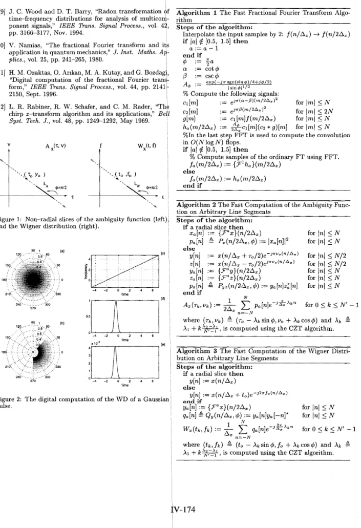
Let us consider the case of computing the samples of the AF ax(^, f ) along the line segment L A shown in Fig. 1 . The following parameterization for the line segment L A will be

used in the derivations: I

L A = ( ( r , v ) ~ ~ = ~ , - A s i n + , v = v , + ~ c o s ~ , ~ ~ AI,^]} 1, where ( T , , V ~ ) is an arbitrary point which lies on L A and

q5

+

r / 2 is the angle between L A and r-axis. Using this

parameterization of L A and the definition of the AF, the non- radial slice of the AF which lies on the line segment L A can be written as

A , ( ~ , - A s i n @ , v , + X c o s ~ ) rA E , ( X , @ + n / 2 )

,

(10) where A;, (A, 4+7r/2) is the radial slice of the cross-ambiguity function of the following time-domain signals y(t) and

~ ( t )

y(t) =

z ( t

+

~ ~ / 2 ) e - ~ ~ ~ ~ ~

( W

z ( t ) =

z ( t

.

Thus, the non-radial slice of AX(7,v) is equal to the radial

slice of the Aye(r, v) where both of the two slices are in paral- lel. Hence, using (8) and (9) in ( l o ) , we obtain the following expression for the non-radial slice of the AF Ax(r, Y ) :

A,(T,- Asin+,vo

+

Acos+) = ya(r)z:(r)e-32TrXdT. (12) To obtain a form suitable for digital computation, we will replace the above integral with its uniform Riemann summation. For an equally valid approximation at all angles

4,

in the rest of this paper, we assume that prior to obtain its samples, z ( t ) is scaled so that the Wigner domain supports of

z ( t ) ,

y(z) and z ( t ) are approximately confined into a cir- cle with radius A,/2 centered at the origin. For z ( t ) with approximate time and band-width of

(At)

and (A,) respec- tively, the required scaling is z ( t / s ) where s = Ill].

After the scaling, the band-width of the signal ya(r)z; ( T )

is given as 2Ax. Therefore the integral (12) can be approxi- mated with a discrete-Fourier transformation. This discrete- Fourier transformation relation can be further discretized (in the variable A) to obtain the following expression for the

N'

uniformly spaced samples of AF on the line segment

L A :

s

where ( ~ k , vk)

4

(T, - A k sin+, v,

+

~k COS^), A k

k

+

After the discretization, the obtained form lends itself for an efficient digital computation since the required samples of the FrFTs, ya(n/2Ax), za(n/2AX), - N

5

n

5

N , can

be computed using the recently developed fast computation algorithm [ll] in O(N1ogN) flops', and the summation in

(13) can be computed in O ( N log N ) flops' using the chirp- z transform algorithm [12]. Therefore the overall cost of computing the samples of the AF along any line segment is O(N1og N) flops.

k X 2 - X _{for 0}

₅

_k

₅

_N'_-_{1 and}_N

₂

_{A: is an integer.}

4 Fast Computation

of the

Wigner Dis-

tribution on Arbitrary

Line

Segments

In the rest of this paper, we will present the dual development for the Wigner distribution. In the next section we introduce the dual of the Radon Wigner Ti-ansform: the Radon- Ambiguity Function Transform (RAFT). Then, we derive the relationship between the RAFT and FrFT. As in the computation of AF samples, this relationship will naturally lead us to the fast computation algorithm for the required WD samples.

Complex multiplication and addition.

2The computational complexity is given for N'

5

N , which is usually the case.

(3)

4.1 Radon-Ambiguity Function Transform

We introduce the Radon-Ambiguity Function Transform of a signal y ( t ) as the Radon transform of its ambiguity function:

Q y ( r , $ )

= /

A , ( r c o s $ - s s i n + , r s i n $ + s c o s + ) d s

,

(14) Using the projection-slice theorem, the radial slice of the WD at an angle q!+.rr/2 can be written as the FT of Q y ( r ,

4)

with respect to the variable r:

1

Q y ( r , q4)e--32rrx dr = W,”(X,

4 +

7r/2)

,

(15) where W,”(X,4) !iW,(Xcos$, Asin$) is the polar representa- tion of the WD. Also, an important relationship between the RAFT and the FrFT can be derived, by substituting (3) into (15) and then making a change of the integration variables:

Q y ( r , 4 ) = y a ( r / 2 ) d ( - r / 2 ) for a =

-4

. (16) In the following section, based on the above relationships we propose an efficient algorithm to compute samples of the WD on arbitrary line segments.

2

7r

4.2 Computation

of

the Wigner Distribu-

tion Along Arbitrary Line Segments

Suppose that we want to compute samples of the WD of a waveform z ( t ) , along an arbitrary line segment Lw as shown in Fig. 1. Since the line segment LW may not pass through the origin, we cannot immediately use the results of the previous section. However, as in Section 3.2, what we will do is to express the required non-radial slice as the radial slice of the WD of an other function which allows us to use the results of the previous section.

In the following derivation we parameterize the line segment LW as:

LW = { ( t , f)lt =

to

- Xsin

4,

f

= fo

+

X cos q5, X E

[XI,

A,])

In this expression ( t o , fo) is an arbitrary point which lies on

LW and

4 +

7r/2 is the angle of LW with the t-axis. Using this parameterization of L w , the non-radial slice of the WD can be expressed as

Wz(to -Xsin$,fo+Xcos$) W,(-Asin$,Xcos$)

,

(17) where y ( t ) = z(t+t,)e-32“fot and W,(-Xsin$,Xcos$) is the radial slice of the WD of y(t). By using the projection-slice theorem given in (15), we obtain the non-radial slice of the WD as

W,(to-Xsin4,Xcos4+fo) = Q ? , ( r , ~ ) e - - 3 2 n r x d r , (18) where Q y ( r ,

4)

is the $-Radon projection of the Wigner distribution W Y ( t , f ) . Since the required $-Radon projection satisfies the FrFT relationship given in (16), it can be efficiently computed by using the fast FrFT algorithm given in Algorithm 1. The details of the O(N1ogN) algorithm is given in Algorithm 3. Note that, unlike P y z ( r , $) which is the $-Radon projection of the CWD given by (7), the bandwidth

I

of Q y ( r ,

4)

is A,.

5 Simulations

In this section we illustrate the accuracy of the algorithms in digitally computing the WD of a Gaussian pulse. The plots (a) and (b) in Fig. 2 are obtained by repeated application of the Algorithm 3. In plot (a) the WD is computed over a full and in plot (b) it is computed over a partial polar grid. To show the accuracy of the proposed algorithm, we computed samples of the Wigner distribution of the same Gaussian pulse over the non-radial line-segment shown in Fig. 2.(c). The obtained samples and the approximation error are plotted in (d) and (e) respectively.

6 Conclusions

Based on the relationship of Wigner distribution and ambiguity function with the fractional Fourier transformation, efficient algorithms are proposed for the computation of Wigner distribution and ambiguity function samples on arbitrary line segments. The proposed algorithms make use of an efficient computation algorithm of fractional Fourier transformation to compute N uniformly spaced samples in O(N1og N) flops. The ability of obtaining samples on arbitrary line segments provides significant freedom in the shape of the grids used in the Wigner distribution or in ambiguity function computa- tions. The proposed algorithms are potentially very useful in the development of new approaches for the analysis, filtering and synthesis of signals.

References

[l] T. A. C. M. Claasen and W. F. G. Mecklenbrauker, “The Wigner distribution - A tool for time-time frequency

signal analysis, Part ii: Discrete-time signals,” Philaps

J . Res., vol. 35, pp. 276-350, 1980.

[2] T. A. C. Claasen and W. F. G. Mecklenbrauker, “The aliasing problem in discrete-time Wigner distributions,”

IEEE Trans. Acoust., Speech, and Signal Process.,

vol. 31, pp. 1067-1072, Oct. 1983.

[3]

L.

Cohen, “Time-frequency distributions - A review,”

Proc. IEEE, vol. 77, pp. 941-981, July 1989.

[4] P. M. Woodward, Probability and Information Theory, with Applications t o Radar. New York: Pergamon Press Inc., 1953.

[5] C. H. Wilcox, “The synthesis problem for radar ambiguity functions,” MRC Technical Summary Report 1957, Apr. 1960.

[6] R.

E.

Blahut, W. Miller, and

J. C.

H. W. ??, Radar and

Sonar, vol. 32. Springer-Verlag, 1991.

[7] J.

C.

Wood and D. T. Barry, “Tomographic time- frequency analysis and its application toward time- varying filtering and adaptive kernel desing for multicomponent linear-fm signals,” IEEE Trans. Signal Pro- cess., vol. 42, pp. 2094-2104, Aug. 1994.

[8] J . C. Wood and D. T. Barry, “Linear sinal synthesis using the Radon-Wigner trasnform,” IEEE Trans. Signal

Process., vol. 42, pp. 2105-2166, Aug. 1994.

(4)

(91 J. C. Wood and D. T. Barry, "Radon transformation (

time-frequency distributions for analysis of multicon ponent signals," IEEE 71-ans. Signal Process., vol. 4: pp. 3166-3177, NOV. 1994.

[lo] V. Namias, "The fractional Fourier transform and ii application in quantum mechanics," J . Inst. Maths. Aj

plies., vol. 25, pp. 241-265, 1980.

[ll]

H.

M. Ozaktas,

0.

Arikan, M. A. Kutay, and

G.

Bozdag "Digital computation of the fractional Fourier trani form," IEEE Tbans. Signal Process., vol. 44, pp. 2141 2150, Sept. 1996.

[12] L. R. Rabiner, R. W. Schafer, and C. M. Rader, "TI chirp z-transform algorithm and its applications," BE

Syst. Tech. J., vol. 48, pp. 1249-1292, May 1969.

V

t

Figure 1: Non-radial slices of the ambiguity function (left and the Wigner distribution (right).

-.. . ,. 270 240" ..., :, .. ..''300 '. . -. 240". ..., :...."'300 270

F

- 0

gLzTc)

- 4 - 2 0 2 4 6 time ,

.

(4

'I

I1

_{I \}

time

Figure 2: The digital computation of the WD of a Gaussia pulse.

A l g o r i t h m 1 The Fast Fractional Fourier Transform Algo-

S t e p s of the algorithm:

Interpolate the input samples by 2: f ( n / A , )

-+

f(n/2A,) if la1

$

[0.5, 1.51 then end if

4

:= E a a : = a - 1

a

:= c o t 4

p

:= csc4 A$ := exp(--jn sgn(sin $ ) / 4 + j @ / 2 )

% Compute the following signals: .-

.-

e3*(a-P)(m/2A,)z for

lml

5

N

c2 [ml

._

.-

e3r0(.m/2A,)2 for Iml

I

2N

gIm1 := ~;[m]f (m/2&) for Jml

5

N

h,(m/2A,) := &cl[m](cz * g ) [ m ] for ImJ

I

N

%In the last step F F T is used to compute the convolution in O ( N log N ) flops.

if

Jal $! [0.5, 1.51 then

I s i n @ l l / 2

c1 [ml

% Compute samples of the ordinary F T using FFT. fa(m/2Ax) := {F1h,}(m/2A,)

fa(m/2At) := ha(m/2Az) else

end if

Algorithm 2 The Fast Computation of the Ambiguity Func- tion on Arbitrary Line Segments

S t e p s of t h e algorithm: i f a radial slice then

za[n] := {Faz}(n/2Az)

1

'"

A~(TI,,vI,) :=

-

pa[n]e-3&";-Xn

2Ax n=-N

for 0

5 IC

5

N ' - 1

where (TI,, VI,)

XI

+

k w ,is computed using the CZT algorithm.

(ro -

XI,

sin

4,

v,

+

XI, cos

4)

and XI,

Algorithm 3 The Fast Computation of the Wigner Distri- bution on Arbitrary Line Segments

S t e p s of the algorithm:

if a radial slice t h e n y[n] := .(n/A,) else

y[n;] := z(n/A,

+

t,)e-32"fo(n/Az)

end if

pa[.] := {Faa}(n/2Az) for

In/

5

N

where ( t k , f k )

A1

+

k

w

,

is computed using the CZT algorithm.

(to

- X I , sin

4,

f0

+

X I , cos

4)

and X I ,

4