Full Terms & Conditions of access and use can be found at
http://www.tandfonline.com/action/journalInformation?journalCode=tprs20
Download by: [Bilkent University] Date: 13 November 2017, At: 03:05
ISSN: 0020-7543 (Print) 1366-588X (Online) Journal homepage: http://www.tandfonline.com/loi/tprs20
Cellular manufacturing system design using a
holonistic approach
M. Selim Akturk & Ayten Turkcan
To cite this article: M. Selim Akturk & Ayten Turkcan (2000) Cellular manufacturing system design using a holonistic approach, International Journal of Production Research, 38:10, 2327-2347, DOI: 10.1080/00207540050028124
To link to this article: http://dx.doi.org/10.1080/00207540050028124
Published online: 14 Nov 2010.
Submit your article to this journal
Article views: 100
View related articles
INT
.
J.
PROD.
RES.,
2000, VOL.
38, NO.
10, 2327 ± 2347Cellular manufacturing system design using a holonistic approach
M. SELIM AKTURK{* and AYTEN TURKCAN{
We propose an integrated algorithm that will solve the part-family and machine-cell formation problem by simultaneously considering the within-machine-cell layout prob-lem. To the best of our knowledge, this is the ® rst study that considers the e ciency of both individual cells and the overall system in monetary terms. Each cell should make at least a certain amount of pro® t to attain self-su ciency, while we maximize the total pro® t of the system using a holonistic approach. The proposed algorithm provides two alternative solutions; one with independent cells and the other one with inter-cell movement. Our computational experiments indicate that the results are very encouraging for a set of randomly generated problems.
1. Introduction
Group technology (GT) is an innovative approach to batch-type production which seeks to rationalize small-lot production by capitalizing on the similarities that exist among component parts and/or processes. GT tries to bring the bene® ts of mass production to high variety, medium-to-low volume quantity production. GT has several bene® ts such as reduced material handling, work-in-process inventory, setup time and manufacturing lead time, and simpli® ed planning, routing and sched-uling activities. The application of GT to manufacturing is cellular manufacturing (CM) which is the physical division of the manufacturing facilities into production cells, representing the basis for advanced manufacturing systems such as just-in-time, ¯ exible manufacturing system and computer integrated manufacturing. In the part-family and machine-cell formation (PFMCF) problem, machines are grouped into cells to produce a group of parts having similar design attributes or manufacturing requirements.
Cellular manufacturing system (CMS) design problem is very important, but complex in nature. In literature, di erent approaches are proposed to solve the CMS design problem. O odile et al. (1994) provide a comprehensive review of the CM literature. The most popular method is called the matrix formulation technique, which uses the binary machine-part incidence matrix as an input and process on it by rearranging rows and columns according to some measures until visible clusters are formed. The most common objective is to minimize the inter-cell movements and inter-cell material handling costs. Although, the real impact of inter-cell and intra-cell moves cannot be realistically determined without knowing the production vol-umes, operation sequences and cellular layout. For example, the parts with high volumes cause more moves, whereas an intermediate operation in a cell can cause
International Journal of Production Research ISSN 0020± 7543 print/ISSN 1366± 588X online#2000 Taylor & Francis Ltd http://www.tandf.co.uk/journals
Revision received September 1999
{ Department of Industrial Engineering, Bilkent University, 06533 Bilkent, Ankara, Turkey.
* To whom correspondence should be addressed.
two inter-cell moves while the ® rst or the last operation causes only one move. Furthermore, the existing studies usually assume that the available machine capa-cities are enough for producing all the parts, consequently an in® nite capacity may not be a realistic assumption in most real-life cases. Moreover, if an additional machine investment cost is justi® ed then additional machines can be bought to reduce inter-cell material handling costs, and ultimately to achieve the cell indepen-dence. Therefore, the available machine capacities, processing times and production volumes should be included in the design process to calculate the required machine capacities. Several mathematical programming models are formulated for the PFMCF problem. These models usually cannot be solved in reasonable computation times, but they can be used to provide insights into the development of good heur-istic methods. Local search heurheur-istics such as simulated annealing, tabu search and genetic algorithms are proposed to solve the mathematical programming models (Heragu and Gupta 1994, Joines et al. 1996, and Vakharia and Chang 1997).
In several studies, it is assumed that each part has only one ® xed route, except the studies by Choobineh (1988), Ho and Moodie (1996), Adil et al. (1996), Beaulieu et
al. (1997) and Askin and Zhou (1998). When each part has only one routing, the
creation of independent cells may not be possible without buying additional machines or allowing inter-cell moves. In most of the manufacturing ® rms, the parts usually have alternative routes. Furthermore, in the existing literature, the part-family formation process is usually made independent of the machine-cell for-mation process. In other words, there is no consideration of how the machines will be arranged within the cell, how the materials move in a cell, and how much machine investment is required to process the parts assigned to that cell. There are few studies that consider the GT layout problem such as Vakharia and WemmerloÈv (1990), Dahel (1995), Verma and Ding (1995), Akturk and Balkose (1996), and Bazargan-Lari and Kaebernick (1996). Therefore, the con® guration and the performance measures of the cell must be considered throughout the design process in order to provide information for the selection of the best part-family and machine-cell for-mation and spatial arrangements of machines in each cell.
Every ® rm should make pro® t to stay in the market. In most of the studies, one or more of the manufacturing costs; variable production cost, setup cost, inter-cell and intra-cell material handling costs, or additional machine investment cost, are tried to be minimized while solving the PFMCF problem. The cost minimization objective is an important one when we consider the overall system performance. Although it causes a kind of dependency between cells when the performance of the individual cells is of concern. For example, a cell that is loosing money is dependent on another cell making pro® t. Therefore, we employ a holonistic approach to solve CMS design problem by considering both the performance of individual cells and the overall system. A holonistic manufacturing system (HMS) is a system of holons that can cooperate to achieve a common goal or objective. `Holon’ is an identi® able part of a system that is made up of subordinate parts and has a unique identity. They are autonomous and cooperative building blocks of the system. The holonic organization enables the construction of very complex systems that are e cient in the use of resources, highly resilient to external and internal disturbances and adaptable to changes as discussed in HoÈpf (1994). There are several similarities between HMS and CMS. CMS design starts with forming cells which are similar to holons in HMS. In HMS, the holons have tasks to perform. In CMS, part families and machine groups are formed to determine the tasks of cells. The main
di erence between the traditional cellular manufacturing systems and HMS is the autonomy of the entities in HMS. Autonomy, which is the capability of an entity to create and control its own plans and strategies, is mostly not found in cells in CMS. We introduce the autonomy concept to the CMS design problem to form self-su cient cells.
The remainder of the paper is organized as follows. In section 2, we de® ne the scope of the study with underlying assumptions and state a mathematical formula-tion of the problem. In secformula-tion 3, we present the proposed soluformula-tion procedure, which is applied in an example problem in section 4. The results of the experimental design to test the e ciency of the algorithm are discussed in section 5. Finally, some con-cluding remarks are provided in the last section.
2. Problem statement
In this study, our aim is to solve the PFMCF and layout problems simul-taneously using a holonistic approach to maximize pro® t of not only the overall system but also individual cells. While forming cells and determining their within-cell layouts, several important manufacturing issues such as production volumes, processing times, operation sequences, alternative routings and machine utilization levels are incorporated into the design problem. The pro® t maximization objective is inspired from an application to a state-owned manufacturing company in Turkey. The company has divided some part of its factory into small holons in order to implement HMS. Since the company is being privatized, these holons are sold to individuals to form small enterprises. These enterprises produce parts for the company and sell them to the company. They also have the ability to produce for other ® rms. The main characteristics of holons, which are the cooperativeness of entities to achieve common goals and the autonomy of them to create and control their own plans and strategies, seem to exist in these enterprises. But, most of these enterprises face economical problems that limit their autonomy. They cannot make enough pro® t due to low utilization levels and high number of intercell movements. The enterprises should make pro® t to achieve selfsu -ciency and to stay in the market. Therefore, in the proposed algorithm, the e ciency of the individual cells is tried to be achieved with the use of minimum pro® t level for cells. The pro® t of the system, which is a ected by the pro® t of individual holons, is also important for the holons since they cooperate to achieve a common goal. So, pro® t maximization objective together with the low pro® t level constraints are used in this model.
The number of parts and machine types are assumed to be known a priori. Each part has a ® xed demand, alternative routings, and predetermined processing times on each route. Processing times, together with the part volume, are used in determining the number of machines required of each type. The operation sequences of parts are important in determining the within-cell layout. In this study, the machines in the cells are located next to each other in series to form a ¯ ow-line manufacturing cell. If there is more than one machine of the same type assigned to a cell, the duplicate machines are assumed to be located in parallel. The raw material, production, material handling and additional machine invest-ment costs, and selling prices of the parts are assumed to be known. These monetary terms will be included in the pro® t maximization objective. Under these assumptions, part families and routings of parts, machine groups, part
assignments to cells, machine assignments to cells in terms of quantities and the location of machines in each cell will be determined.
We propose a mixed integer programming (MIP) model to maximize the pro® t under cell size, low utilization and low pro® t level constraints while determining the layout, part assignments, routing selections and machine assignments.
The parameters of the problem are as follows:
p number of cells, n number of parts, M set of all machine types, Ri number of routes for part i;
Di demand for part i;
Yirkl 0± 1 binary indicator which is equal to 1 if part i should be processed by
machine type k immediately before machine type l in its rth route,
hi unit material handling cost of part i within a cell,
cirk unit production cost of part i using route r on machine k per unit time,
tirk unit processing time of part i using route r on machine k;
SPi selling price of part i;
RMi raw material cost of part i;
L Pj lower limit for the pro® t of cell j ;
Ak available unit capacity of machine type k;
MAk available number of machine type k;
MCk additional machine investment cost of machine k;
CSj an upper limit on the number of machines assigned to cell j ;
U a very large constant,
Mir set of machines in the rth route of part type i;
®kj lower limit for the utilization levels of machine type k in cell j.
The decision variables are the following:
Xirj 0± 1 binary variable which is equal to 1 if part i is allocated to cell j
using the rth route,
mkj 0± 1 binary variable which is equal to 1 if machine k is allocated to cell j ;
mlkj location of machine k in cell j;
S‡
klj;Sklj¡ number of skippings and backtrackings between machines k and l in
cell j ;
¬klj 0± 1 binary variable which is equal to 1 if machine l is placed after (not
necessarily immediately) machine k in cell j ;
¯irjkl 0± 1 binary variable which is equal to 1 if part i uses route r and
allocated to cell j, where machine k is not located immediately before machine l,
¶j 0± 1 binary variable which is equal to 1 if cell j is opened,
Nkj number of type k machines assigned to cell j,
MNk number of additional machines of type k needed.
A MIP formulation of the problem is as follows: . Objective function
Maximize X n iˆ1
…
SPi¡ RMi†
¢ Di¢ X r2Ri Xp jˆ1 Xirj…
†
" # ¡ X p jˆ1 Xn iˆ1 X r2Ri X k2Mir X l2Mir Di¢ hi¢ ¯irjkl " # ¡ X p jˆ1 Xn iˆ1 X r2Ri X k2MirDi¢ cirk¢ tirk¢ Xirj
" # ¡ X k2M MCk¢ MNk " # :
. Part and machine allocation, and routing selection constraints
Xp jˆ1 X r2Ri Xirjˆ 1 8i
…
1†
X r2Ri Xirjµ
¶j 8i; j…
2†
Xirjµ
mkj 8i;r;j ;k 2 Mir…
3†
mkjµ
¶j 8k; j:…
4†
. Layout related constraints
mkj
¶
mlUkj 8k; j…
5†
mkjµ
mlkj 8k; j…
6†
mlkj¡ mllj‡
U¬klj¶
mkj‡
mlj ¡ 1 8k; l ; j…
7†
mllj¡ mlkj‡
U…
1 ¡ ¬klj†
¶
mkj‡
mlj ¡ 1 8k; l ; j…
8†
S‡ klj¡ S¡kljˆ mllj¡ mlkj 8k; l ; j…
9†
¯irjkl‡
…
1 ¡ Xirj†
¡ S‡ klj¡ 1 2U ¡ S¡ klj U…
†
Yirkl¶
0 8i;r; j;k;l:…
10†
. Low pro® t level constraint
Xn iˆ1 X r2Ri Di¢
…
SPi¡ RMi†
¢ Xirj¡ Xn iˆ1 X r2Ri X k2Mir X l2Mir Di¢ hi¢ ¯irjkl ¡X n iˆ1 X r2Ri X k2MirDi¢ cirk¢ tirk¢ Xirj
¶
L Pj 8j:…
11†
. Low utilization level constraint
Xn
iˆ1
X
r2Ri
tirkDiXirj
¶
®kj 8k; j:…
12†
. Machine capacity constraints (also determines the additional machines needed) Xn iˆ1 X r2Ri tirkDiXirj
µ
NkjAk 8k; j…
13†
Xp jˆ1 Nkj¡ MNkµ
MAk 8k…
14†
mkj¶
Nkj=U 8k; j…
15†
mkjµ
Nkj 8k; j…
16†
. Cell Size constraint
X
k2M
Nkj
µ
CSj 8j:…
17†
. Non-negativity and integrality constraints
Xirj;¶j;mkj;¬klj;¯irjklˆ 0;1
and
mlkj; Nkj;MNk non-negative integers 8i;r; j;k;l:
…
18†
The overall objective is to maximize the total pro® t. The ® rst item in the objective function is the di erence between the revenue and the raw material cost. This term does not change by the cell that the part is assigned or the route selected for the part. The material handling and variable production costs, denoted as the manufacturing cost, are the second and third terms in the objective function, respectively. The material handling cost is incurred to the parts making an intra-cell movement. The variable production cost changes according to the route selected. Since addi-tional machines may be needed to form completely independent cells, the addiaddi-tional machine investment cost, which is the fourth term in the objective function, should be as small as possible.
The ® rst set of constraints satisfy the assignment of each part to only one cell and selection of only one route among alternative routing capabilities. The second and third set of constraints ensure that a part can be assigned to a cell if it is opened and contain all of the machines needed to process the part. Constraints 4, 5 and 6 provide that if a machine is allocated to a cell then the location of the machines should be greater than one. Constraints 7 and 8 ensure the assignment of machines to di erent locations in a cell such that two machines cannot occupy the same place in a cell. Constraint 9 determines the number of skippings and backtrackings between the machines in a cell. In constraint 10, a material handling cost is not incurred when the two consecutive machines in the operation sequence are next to each other in the forward ¯ ow direction. On the other hand, a material handling cost is incurred for the backtrackings and the skippings which are determined according to the order of machines in the cell and the operation sequences of parts. Skippings and backtrack-ings are given equal weights in this problem, since they are both performed by the same type of material handling equipment. The cells should make at least a prede-termined amount of pro® t which is satis® ed by constraint 11. This comes from the holonistic view to form autonomous, self-su cient cells. Constraint 12 allows the
decision makers to specify a lower limit on the desired machine utilization in a cell. Constraint 13 determines the number of machines of each type required in each cell. Constraint 14 ® nds the number of additional machines needed to calculate the additional machine investment cost. Constraints 15 and 16 provide the assignment of a machine to a cell if it is needed in that cell. There are several physical constraints, such as two machines cannot occupy the same place in a cell as discussed above. Another one could be space limitations. Therefore, the size of a cell is often deter-mined by the ¯ oor area of the factory which sets an upper limit on the number of machines a cell can have. The size of the cell should be a reasonable one to make the controlling, scheduling, and planning activities easier in the cell, which is ensured by constraint 17.
3. Algorithm
A local search heuristic is proposed to solve the problem in a reasonable com-putation time to form completely independent cells. The proposed algorithm has three main stages. The ® rst two stages are used to ® nd a solution to the main prob-lem (MP). Since the inter-cell movements are also important for reducing the addi-tional machine investment cost, the assumption of forming completely independent cells can be relaxed in the algorithm. In the third stage, inter-cell movements are introduced to decrease additional machine investment cost, hence improve the objec-tive function value.
Stage 1: Finding an initial solution
In the proposed algorithm, the ® rst stage is the construction of an initial solution. In this stage, the within-cell layout and low utilization level constraints are relaxed, and the layout related constraints, non-negativity and integrality constraints of MP (constraints 5± 10, and 18) are replaced with the following constraints to form a new subproblem. mkj¡ X l2M lkj
¶
0 8k; j…
19†
mkj¡ X l2M klj¶
0 8k; j…
20†
mkj¡ X l2M klj¡ X l2M lkjµ
0 8k; j…
21†
…
¯irjkl¡ Xirj‡
klj†
Yirkl¶
0 8i;r; j;k;l…
22†
Xirj;¶j;mkj;klj ˆ 0;1 and Nkj are integers 8i;r; j ;k;l:
…
23†
where klj is equal to 1 if machine k is placed just before machine l in cell j and 0
otherwise.
The constraints of the subproblem are 1± 4, 11± 17, and 19± 23. The disadvantage of the new layout related constraints is that the locations of machines in the cell cannot be determined exactly. We can only ® nd the machines next to each other, hence the ® nal layout can be infeasible. The same type of machine can be duplicated at the beginning and at the end of a group of machines in a cell without incurring an additional machine investment cost. The computational time needed to solve sub-problem is signi® cantly less than the time needed to solve the MP. In the main problem, mlkj’s should be de® ned as integers and ¯irjkl’s as binary variables. MP
has additional
…
3m‡
2†
£ m £ p constraints, m £ p integer and n £ p £ R £…
NOP ¡ 1†
binary variables. R is the average number of routes for parts and NOP is the average number of operations in a part’s sequence. After the layout constraints are replaced, the low utilization level constraint is also relaxed to reduce the com-putation time even further. The relaxed subproblem (RSP) can be solved optimally in a reasonable time for small problems, although it may or may not be feasible for MP, since the layout and low utilization level constraints are relaxed. If the solution is infeasible for MP, then stage 2 is used to ® nd a feasible solution. The steps of stage 1 are as follows:1.1 Form RSP and solve it by using the CPLEX software to ® nd an initial solution. The current solution (CS) is the solution found by solving RSP.
1.2 Determine the layout found by RSP. Calculate the utilization level of each machine in each cell by Utilkj ˆPiPr2RitirkDiXirj. If either the layout is
infea-sible or low utilization level constraint is not satis® ed then the solution is in-feasible for MP, go to stage 2. Else, go to stage 3 if any additional machine investment is required to form completely independent cells.
Stage 2: Formation of independent cells
In the second stage, alternative solutions are constructed by assigning parts to other cells and/or selecting alternative routes for parts to ® nd a feasible solution to the MP. The promising alternatives are found by calculating the change in the objective function value and one promising alternative is selected randomly to per-turb the solution. The procedure continues by searching the neighborhood of the current solution until a stopping criterion is reached. The criteria can be ® nding either a feasible solution or reaching to a maximum limit on step size, or having no further improvement in the objective value. In the next step, the feasible solution is tried to be improved by continuing local search. These steps are performed for a number of iterations to reduce the e ect of randomness in selecting the alternatives. While performing the local search, the feasible solution giving the best objective value is kept as an incumbent solution to the proposed mathematical model. The steps of stage 2 are as follows:
2.1 If the layout of cells are found to be infeasible for MP in stage 1, determine alternative layouts for each cell.
2.2 Take an initial layout for each cell. Update CS in terms of layout.
2.3 CS0ˆ CS. For CS0, calculate utilization levels of machines in each cell and total pro® t of each cell (TPj), such that T Pjˆ SPRMj¡ V PCj¡ MHCj, where
MHCjˆ X i X r2Ri X k2MRir X l2MRir hi¢ Di¢
…
1 ¡ klj†
¢ Xirj V PCjˆ X i X r2Ri X k2MRircirk¢ tirk¢ Di¢ Xirj
SPRMjˆ X i X r2Ri
…
SPi¡ RMi†
¢ Di¢ Xirj:If either low pro® t level constraint or low utilization level constraint is not satis® ed go to step 2.4, else go to step 2.5.
2.4 Search the neighborhood of CS0 to ® nd a feasible solution.
2.4.1 Find the alternative parts that can be assigned to other cells and the corresponding promising cells to which the alternative parts can be assigned. If machine k in cell j violates the low utilization level con-straint, the parts using this machine in cell j and the parts using the machine of the same type in other cells are candidates that can be assigned to other cells. A promising cell, to which an alternative part can be assigned, contains a certain percentage of machines in a part’s routing denoted by ³, and satis® es the following condition
…
NOPi¡ # machines needed†
=NOPi¶
³.2.4.2 For each alternative, determine the within-cell layout and calculate the corresponding cost terms in cells. When part i using route r in cell j is assigned to cell j j and produced with its rrth route, the cost terms change as follows: New MHCj0 ˆ X i X r2Ri X k2MRir X l2MRir hi¢ Di¢
…
1 ¡ klj0†
¢ Xirj0; for j0ˆ j ; j j New V PCjˆ Old V PCj¡ X k2MRi;r cirk¢ tirk¢ Di New V PCj jˆ Old V PCj j‡
X k2MRi;rr ci;rr;k¢ ti;rr;k¢ Di New SPRMjˆ Old SPRMj¡…
SPi¡ RMi†
¢ Di New SPRMj jˆ Old SPRMj j‡
…
SPi¡ RMi†
¢ DiNew TPj0 ˆ New SPRMj0¡ New V PCj0¡ New MHCj0;
for j0ˆ j ; j j:
If the cells j and j j do not violate the low pro® t level constraints, the change in the objective function value for the alternative
…
i;rr;j j†
is calculated as follows:D
Obji;rr;j jˆ New TPj¡ Old TPj‡
New T Pj j¡ Old T Pj j‡
MIC1 ¡ MIC2;where MIC1 is the money spend for the machines which are not needed anymore and MIC2 is the total cost needed to buy the new required machines.
2.4.3 Form a restricted candidate list (RCL). Every alternative
…
i0;rr0;j j0†
is added to the RCL if it satis® es the following condition of…
maxi;rr;j jfD
Obji;rr;j jg ¡D
Obji0;rr0;j j0†
µ
…
·¢ Obj†
, where · is a prede® nedparameter to select the promising alternatives. Select one alternative from the list randomly and update CS0. According to the selected alter-native,
…
i*;rr*;j j*†
, part i* is produced in cell j j* with its rr*th route, and the objective value is updated as New Obj ˆ Old Obj‡
D
Obji¤;rr¤;j j¤.2.4.4 Repeat steps 2.4.1± 2.4.3 until a stopping criterion is reached. The stop-ping criteria are ® nding a feasible solution or reaching to the maximum step size.
2.5 Try to improve the feasible solution by searching the neighborhood of the current solution. This step is similar to the previous step except that determina-tion of alternative parts and the stopping criteria di ers. All parts are candi-dates that can be assigned to other cells. The stopping criteria are having no further improvement in the objective function value or reaching to the maxi-mum step size.
2.6 Repeat steps 2.3± 2.5 for a ® xed number of iterations.
2.7 Repeat steps 2.2± 2.6 until all alternative layouts are evaluated.
2.8 Best feasible solution is reported as the ® nal solution. If any additional machine investment is required to form completely independent cells, then go to stage 3. Stage 3: Allowing inter-cell movements
At the end of second stage, an additional investment might have been made for some machines to form completely independent cells. Decision maker may allow some inter-cell movements to reduce the additional machine investment cost. Inter-cell movements can also increase the overall pro® t by giving a better material ¯ ow, although they complicate the scheduling within cells. While inter-cell movements are allowed, the objective of forming pro® table cells is not violated. An important dis-tinction from a typical minimization of inter-cell movements objective is the alloca-tions of pro® t and manufacturing costs between the interacted cells. While calculating the material handling cost, the intra-cell movement costs are incurred to the cell in which the intra-cell movement takes place. The inter-cell movement costs are incurred to the cell to which the part is assigned. The variable production cost for each operation is incurred to the cell in which this operation is performed. The di erence between the revenue and the raw material cost, denoted as gain, is divided between two cells. The gain for each cell is proportional with the variable production cost incurred for the part in that cell. At the end of this stage, cells having interaction with each other via inter-cell moves are formed. The steps of stage 3 are as follows.
3.1 Take the best solution obtained at the end of stage 2 as an initial solution. 3.2 Determine the alternative parts that can make an inter-cell movement and their
corresponding cells. Parts, which are not making an inter-cell movement but require an additional machine investment, are allowed to make an inter-cell movement. Parts can be assigned to their promising cells as in step 2.4.1. The operations that cannot be performed in the promising cell are performed in another cell to which alternative part can make an inter-cell movement. 3.3 When part i, which was using its rth route in cell j, is assigned to cell j j, and
allowed to make an inter-cell movement to cell j j j in order to be processed with its rrth route, the cost terms change as follows:
New MHCjˆPiPr2Ri [(# inter-cell moves
†
¢ Hi‡
…
# intra-cellmoves
†
¢ hiŠ
¢ Di¢ Xirj.New MHCj j ˆ Old MHCj j
‡
…
# inter-cell moves†
¢ Hi¢ Di‡
…
# intra-cellmoves
†
¢ hi¢ Di:New MHCj j jˆ Old MHCj j j
‡
…
# intra-cell moves†
¢ hi¢ Di.New V PCjˆ Old V PCj¡ PCi;r.
New V PCj j ˆ Old V PCj j
‡ ‰
Pk2MRi;rr production cost on machine k if theoperation on machine k is performed in cell j j, denoted as W IPi;rr;j j].
New V PCj j jˆ Old V PCj j j
‡ ‰
Pk2MRi;rr production cost on machine k if theoperation on machine k is performed in cell j j j
Š
: New SPRMjˆ Old SPRMj¡ T SPi.New SPRMj jˆ Old SPRMj j
‡
W IPPCi;rr;j j i;rr ¢ T SPi.New SPRMj j jˆ Old SPRMj j j
‡
PCi;rrPC¡ W IPi;rr;j j i;rr ¢ TSPi.
T Pj0ˆ New SPRMj0¡ New V PCj0¡ New MHCj0, for j0ˆ j, j j, j j j.
If low pro® t level constraint is satis® ed by cells j, j j and j j j, the change in objective function value for alternative (i;rr;j j;j j j) can be calculated as fol-lows:
D
Obji;rr;j j;j j jˆ New TPj¡ Old T Pj‡
New T Pj j¡ Old T Pj j‡
New T Pj j j¡ Old TPj j j‡
MIC1:3.4 Form the RCL as it is explained in step 2.4.3. If no alternative can be found, go to step 3.5. Otherwise, select one of the alternatives from the candidate list randomly. According to the selected alternative, say (i*;rr*;j j*;j j j*), the solution is updated. In the current solution, part i* makes inter-cell movement between cells j j* and j j j* to be processed with its rr*th route. Return back to step 3.2.
3.5 Repeat steps 3.1± 3.4 for a ® xed number of iterations.
3.6 While performing all these steps, the solution giving the best objective value is kept as the incumbent solution.
3.7 Form a from-to-chart by using the number of inter-cell moves and production volumes. The total number of inter-cell moves from cell j j to j j j is equal to Pn
iˆ1
…
# inter-cell moves from cell j j to j j j†
¢ Di. Note that the from-to-chart isnot symmetric. Form a cost chart considering the inter-cell material handling costs between cells. Find the area of each cell by considering the machines assigned to them. The machines of di erent types are located in series in a ¯ ow line, whereas the duplicate machines are located in parallel. If there is not enough space in the factory, the same type of machines can be located next to each other in series. Find the spatial arrangement of cells in the factory by using the CRAFT algorithm.
4. Numerical example
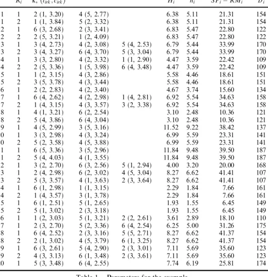
A numerical example is provided to clarify the basic steps of the algorithm. The routing, processing time, production cost, inter-cell and intra-cell material handling costs, the di erence between selling price and raw material cost, and demand of each part can be seen in table 1. Furthermore, the additional investment cost and the available number for each machine type are given in table 2. The minimum pro® t level for each cell is taken as 746.
As discussed earlier, the ® rst stage of the algorithm is used to ® nd an initial solution. The relaxed subproblem is solved by CPLEX. The layout of each cell, the parts (i) assigned to the cells and the routings selected for the parts (r) can be seen in table 3, and the objective function value is 10 392. Although the utilization level constraint is satis® ed by all machines, the layout of cells are infeasible for MP.
i Ri k,…tirk; cirk† Hi hi SPi¡ RMi Di 1 1 2 (1, 3.20) 4 (5, 2.77) 6.38 5.11 21.31 154 1 2 1 (1, 3.84) 5 (2, 3.32) 6.38 5.11 21.31 154 2 1 6 (3, 2.68) 2 (3, 3.41) 6.83 5.47 22.80 122 2 2 2 (5, 3.21) 1 (2, 4.09) 6.83 5.47 22.80 122 3 1 3 (4, 2.73) 4 (2, 3.08) 5 (4, 2.53) 6.79 5.44 33.99 170 3 2 3 (4, 3.27) 6 (4, 3.70) 5 (3, 3.04) 6.79 5.44 33.99 170 4 1 3 (3, 2.80) 4 (2, 3.32) 1 (1, 2.90) 4.47 3.59 22.42 109 4 2 2 (5, 3.36) 1 (5, 3.98) 6 (4, 3.48) 4.47 3.59 22.42 109 5 1 1 (2, 3.15) 4 (3, 2.86) 5.58 4.46 18.61 151 5 2 3 (5, 3.78) 4 (3, 3.44) 5.58 4.46 18.61 151 6 1 2 (2, 2.83) 4 (2, 3.40) 4.67 3.74 15.60 134 7 1 6 (4, 2.62) 4 (2, 2.98) 1 (4, 2.81) 6.92 5.54 34.63 158 7 2 1 (4, 3.15) 4 (3, 3.57) 3 (2, 3.38) 6.92 5.54 34.63 158 8 1 4 (1, 3.21) 6 (2, 2.54) 3.10 2.48 10.36 121 8 2 5 (4, 3.86) 6 (4, 3.04) 3.10 2.48 10.36 121 9 1 4 (5, 2.99) 3 (5, 3.16) 11.52 9.22 38.42 137 10 1 3 (3, 2.98) 4 (3, 3.24) 6.99 5.59 23.31 141 10 2 5 (2, 3.58) 4 (5, 3.88) 6.99 5.59 23.31 141 11 1 6 (5, 3.36) 3 (5, 2.96) 11.84 9.48 39.50 187 11 2 5 (4, 4.03) 4 (1, 3.55) 11.84 9.48 39.50 187 12 1 3 (2, 2.70) 6 (3, 2.56) 5 (1, 2.94) 4.00 3.20 20.00 168 13 1 2 (4, 2.98) 6 (2, 3.02) 4 (5, 3.04) 8.27 6.62 41.41 107 13 2 5 (3, 3.57) 4 (1, 3.63) 2 (3, 3.64) 8.27 6.62 41.41 107 14 1 6 (1, 2.98) 1 (1, 3.15) 2.29 1.84 7.66 161 14 2 1 (4, 3.57) 3 (1, 3.78) 2.29 1.84 7.66 161 15 1 6 (1, 2.51) 5 (1, 2.65) 1.93 1.55 6.45 149 15 2 5 (1, 3.02) 2 (3, 3.18) 1.93 1.55 6.45 149 16 1 1 (2, 3.03) 5 (1, 3.21) 2 (2, 2.61) 3.61 2.89 18.10 110 17 1 2 (3, 2.70) 5 (2, 3.36) 6 (4, 2.54) 6.25 5.00 31.26 175 18 1 6 (4, 2.52) 2 (3, 3.16) 5 (5, 2.71) 8.27 6.62 41.37 154 18 2 2 (1, 3.02) 4 (5, 3.79) 6 (1, 3.25) 8.27 6.62 41.37 154 19 1 6 (3, 2.61) 5 (4, 2.90) 2 (3, 3.01) 7.11 5.69 35.60 123 19 2 4 (3, 3.13) 6 (1, 3.48) 2 (3, 3.61) 7.11 5.69 35.60 123 20 1 5 (3, 3.48) 6 (4, 2.55) 7.74 6.19 25.81 174
Table 1. Parameters for the example.
Machines 1 2 3 4 5 6
MC 1529 1401 1532 1568 1572 1486
MA 1 1 2 3 1 3
Table 2. Additional investment cost and the available number of machines.
Cell Layout Parts (i;r)
1 6 1 5 6Ð 4 2 3 4 (1,2)(3,1)(4,1)(10,1)(13,2)(14,1)(16,1)(17,1) 2 3 1 4 3Ð 6 5 6 (5,1)(7,2)(9,1)(11,2)(12,1)(15,1)(20,1)
3 6 2 4 6 (2,1)(6,1)(8,1)(18,2)(19,2)
Table 3. Solution of the relaxed problem.
Since the solution is infeasible, we proceed to the second stage to ® nd a feasible solution to the main problem.
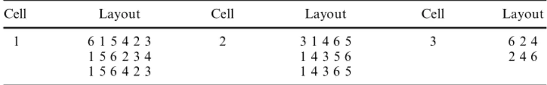
The second stage begins with ® nding alternative layouts for each cell. A limit, 3, on the maximum number of alternative layouts for a cell is used in this example to control the size of the search space. The alternative layouts for each cell can be seen in table 4.
The initial layouts for cells 1, 2 and 3 are taken as (1± 5± 6± 2± 3± 4), (1± 4± 3± 6± 5) and (6± 2± 4), respectively, from the set of alternatives. For the selected initial layouts, total pro® t of cells 1, 2 and 3 are 3222, 4960 and 3153, respectively. The minimum pro® t level constraint is satis® ed and additional machine investment cost is 4502. Although the objective function value of the relaxed problem was 10 392, the objec-tive function value of the initial feasible solution is 6830 due to the increase in material handling cost. At this point, both the low utilization and low pro® t level constraints are satis® ed for the initial solution. Since the current solution is feasible for MP, we have to search the neighborhood of the current solution in order to see whether the solution can be improved or not.
All the parts are denoted as alternative parts since they can be assigned to their promising cells. ³ is taken as 0.3 in this example. The change in objective function value (
D
Obj) is calculated for all alternatives. SinceD
Obj values for somealterna-tives are greater than 0, a restricted candidate list is formed. ·, which determines the size of the RCL, is taken as 0.1. Furthermore, Obj is 6830 and maximum of
D
Objvalues is 1319. Alternatives
…
2;1;1†
, for whichD
Obj ˆ 1319, and…
11;2;4†
, for whichD
Obj ˆ 699, are the only alternatives that can be included in the RCL. Suppose weselect the alternative
…
2;1;1†
from the RCL. Now, part 2 using route 1 is produced in cell 1 and the new objective value becomes 8149. For the current solution, a new set of alternatives are determined and theirD
Obj values are calculated. SinceD
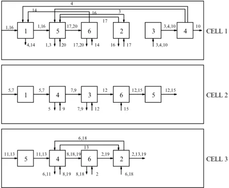
Obj forall alternatives are smaller than zero, we cannot improve the current objective value. The ® rst iteration ends with the stopping criterion of having no alternative left. This search is repeated for a number of iterations until all alternative layouts are evaluated. At the end of this stage, the ® nal solution along with the PFMCF and layout of cells can be seen in table 5. Additional machine investment cost is 6074 and
Obj is equal to 9314. The material ¯ ow in each cell for the ® nal solution can be seen
in ® gure 1, where the numbers on each arc correspond to part numbers, whereas the
Cell Layout Cell Layout Cell Layout
1 6 1 5 4 2 3 2 3 1 4 6 5 3 6 2 4
1 5 6 2 3 4 1 4 3 5 6 2 4 6
1 5 6 4 2 3 1 4 3 6 5
Table 4. Alternative layouts for cells.
Cell Layout Parts (i;r)
1 1 5 6 2 3 4 (1,2)(3,1)(4,1)(10,1)(14,1)(16,1)(17,1)(20,1)
2 1 4 3 6 5 (5,1)(7,2)(9,1)(12,1)(15,1)
3 5 4 6 2 (2,1)(6,1)(8,1)(11,2)(13,2)(18,2)(19,2) Table 5. Final solution without an intercell movement.
nodes denote the machine types. As we can see from the ® gure, all the cells are independent at the end of the second stage.
Since there is an additional machine investment, allowing inter-cell movements may decrease the additional machine investment cost and simplify the material ¯ ow within the cell. The ® nal solution obtained at the end of stage 2 is taken as an initial solution for the third stage, and we try to improve the objective value. The local search begins with ® nding alternatives. Parts, which are not making inter-cell moves and using the machines that should be bought, are candidates to make an inter-cell movement. Additional machine investment cost is made for machines 1, 2 and 5. Parts 1, 2, 3, 4, 5, 6, 7, 11, 12, 13, 14, 15, 16, 17, 18, 19 and 20 are using these machines and they can make an inter-cell movement. For example, part 13 is pro-cessed in cell 3 with its second route. If one of the machines in its routing is used only by part 13, then this machine can be removed from cell 3 and the operation on this machine can be performed in another cell having the required capacity. But there is no such machine in cell 3. The same part can be assigned to another cell and/or can use another routing. Let’s take the ® rst routing of part 13, which is f2;6;4g, and look if it can be assigned to cell 2. In cell 2, machine 2 does not exist. Also, the capacity of machine 4 is not enough, hence two new machines are needed. (NOPi¡ # machines
needed)=NOPiˆ 0:33 is greater than ³ ˆ 0:3. Therefore, part 13 can be assigned to
cell 2 and make an inter-cell movement to cell 1 for the operations on machines 2 and 4, denoted as alternative (13,1,2,1). All parts and cells are evaluated in the same way to ® nd alternative solutions.
D
Obj for all alternatives, (i;rr;j j;j j j), are calculated.The restricted candidate list is formed with maxi;rr;j j;j j jf
D
Obji;rr;j j;j j jg of ¡73:75 andObj of 9314. · is again taken as 0.1. (1,2,3,2), (2,1,2,1), (6,1,2,1), (13,2,1,2), (13,2,2,1),
4 3 14 16 2 6 4 5 11,13 8,18,19 2,19 2,13,19 11,13 8,19 6,11 8,18 2 6,18 6,18 13 1 12,15 5 12,15 15 6 12 12 7,9 3 9 5 4 7,9 5,7 5,7 4 3,4,10 3 3,4,10 2 17 16 6 14 17,20 17,20 17 20 1,3 5 1,16 4,14 1 1,16 10 CELL 1 CELL 2 CELL 3
Figure 1. Material ¯ ow within cells.
(14,1,3,2), (15,1,1,3), (16,1,2,3) and (16,1,3,2) form the set of alternatives in candi-date list with
D
Obj values of ¡982.5, ¡833.75, ¡125.25, ¡885, ¡885, ¡73.75, ¡287.5, ¡397.5 and ¡397.5, respectively. SinceD
Obj ˆ ¡1902 for alternative(13,1,2,1), it is not included to the RCL. Suppose that (14;1;3;2) is selected ran-domly, that means part 14 using route 1 is assigned to cell 3 and allowed to make an inter-cell movement to cell 2. All other part and route assignments remain the same. The new objective function value becomes Obj ˆ 9314 ¡ 73:75 ˆ 9240:25.
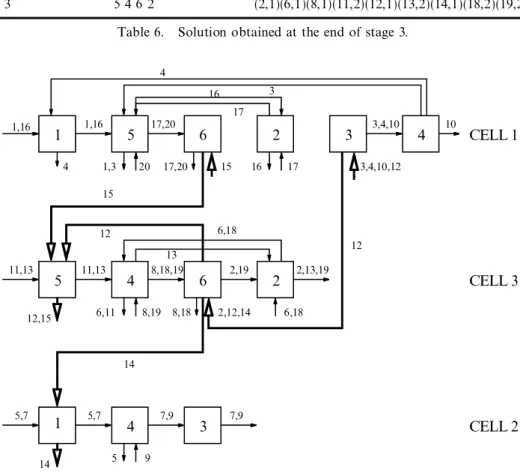
The local search continues until no alternative is left. The search is repeated for a ® xed number of iterations to ® nd di erent solutions to the problem. While perform-ing all these steps, the solution givperform-ing the best objective value is kept as the incum-bent solution. The ® nal solution at the end of stage 3 is given in table 6, where the additional MIC is 4502 and the new Obj is 9316.5. Part 14 makes an inter-cell movement between cells 3 and 2, whereas part 15 between cells 1 and 3, and part 12 between cells 3 and 1. The change in layouts and the material ¯ ow of parts in cells can be seen in ® gure 2. In this solution, the cells have an interaction with each other.
Cell Layout Parts (i; r)
1 1 5 6 2 3 (1,2)(3,1)(4,1)(10,1)(15,1)(16,1)(17,1)(20,1)
2 1 4 3 (5,1)(7,2)(9,1)
3 5 4 6 2 (2,1)(6,1)(8,1)(11,2)(12,1)(13,2)(14,1)(18,2)(19,2) Table 6. Solution obtained at the end of stage 3.
4 3 16 4 4 4 3,4,10 3 2 17 16 6 17,20 17 20 1,3 5 1,16 1 1,16 10 CELL 1 4 17,20 15 3,4,10,12 5 11,13 11,13 1 5,7 5,7 6,11 8,19 5 9 8,18,19 7,9 8,18 2 6 3 6,18 2,13,19 2,19 ,12,14 13 6,18 12,15 14 14 12 15 12 7,9 2 CELL 3 CELL 2
Figure 2. Material ¯ ow within and between cells at the end of stage 3.
The places of cells 2 and 3 are interchanged to decrease the material ¯ ow of parts 12, 14 and 15 as described in step 3.7. Allowing inter-cell movements reduced the addi-tional machine investment cost from 6074 to 4502, hence the total pro® t is increased to 9316.5.
5. Experimental design
We use the C language to code the proposed algorithm. The relaxed MIP sub-problem is solved using CPLEX MIP solver. The code is compiled with Gnu C compiler and the problem is solved on a Sparc Station 10 under SunOS 5.4. There are ® ve experimental factors that can a ect the e ciency of the proposed algorithm, which are listed in table 7. Factor A, the number of parts and machine types, determines the size of the problem. Factor B, the production cost, a ects the route selection decisions. Factor C is the h=C1ratio, where hiis the intra-cell material
handling cost per unit and Ci;1 is the unit production cost of part i per operation
when it is produced with its ® rst route such that Ci;1ˆPk2Mi ;1ci;1;k¢ ti;1;k=NOPi. In
order to evaluate the tradeo s between the material handling costs and acquiring new machines, the variability of additional machine investment cost is used as another factor, Factor D. The ® fth factor, Factor E, corresponds to the H=h ratio, where Hi is the inter-cell material handling cost per unit.
In this study, there are di erent ways of solving the proposed problem: acquiring additional machines or allowing intra-cell moves to retain cell independency, or using alternative routing, or allowing inter-cell moves, or any combination of these strategies. For a given set of cost parameters, tradeo s can be made among these alternative strategies. Therefore, we choose the cost parameters as experimental factors at two di erent levels to see their in¯ uence on the computational results. Moreover, the same material handling equipment usually performs both the intra-cell and inter-intra-cell moves for a certain part. We select these material handling cost terms in a comparable way (Hi> hi) so that we can evaluate di erent strategies in
the proposed algorithm.
Since there are ® ve factors and two levels, our experiment is a 25 full-factorial design, which corresponds to thirty-two treatment combinations. The number of replications of each combination is taken as three producing 96 di erent randomly generated runs. Other variables in the system are treated as ® xed parameters and summarized in table 8, where UN¹
‰
a;bŠ
represents a uniformly distributed random variable in interval‰
a;bŠ
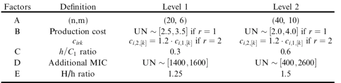
. The number of available machines are determined by considering the machines’ capacities needed to produce all the parts with their ® rst routings. It is known that cell formation problem is sensitive to the maximum number of cells. Therefore, we set p to a reasonably high value so that it does notFactors De® nition Level 1 Level 2
A (n,m) (20, 6) (40, 10)
B Production cost UN ¹‰2:5;3:5Šif r ˆ 1 UN ¹‰2:0;4:0Šif r ˆ 1
cirk ci;2;‰kŠˆ 1:2 ¢ ci;1;‰kŠif r ˆ 2 ci;2;‰kŠˆ 1:2 ¢ ci;1;‰kŠif r ˆ 2
C h=C1 ratio 0.3 0.6
D Additional MIC UN ¹‰1400;1600Š UN ¹‰400;2600Š
E H/h ratio 1.25 1.5
Table 7. Experimental design factors.
Parameters Set of Values Number of operations, NOPi UN ¹‰2; 3Š
Number of routes, Ri UN ¹‰1; 2Š
Processing time, tirk UN ¹‰1; 5Š
Demand, Di UN ¹‰100;200Š
Number of available machines, MAk UN ¹‰»k; »k‡1Šif »kˆ 0; 1
UN ¹‰»k¡ 1; »k‡1Š, otherwise where »kˆ P iDiti1k Ak Cell size, CSj 6
Maximum number of cells, p
P
kMAk
6 ‡3
Available machine capacity, Ak 2000 min/week
Minimum utilization level, ¬kj 0:1 ¤ Ak
Selling price, SPi 1:30 ¢Pk2MRi1ti1k¢ ci1k
Raw material cost, RMi 0:05 ¢Pk2MRi1ti1k¢ ci1k
Minimum pro® t level, L Pj 0:25 ¢ Di…SPi¡ RMi¡Pk2MRi1ci1k¢ ti1k†=p
Table 8. Fixed parameters.
(BCD) Run RSP Objective Final Solution UB* or OPT % GAP (000) 01 26 182 (4.5) 24 677 (1872.6) 24 677 (5639.2) 0.00% 02 14 593 (53.6) 13 975 (194.7) 13 975 (314.9) 0.00% 03 16 093 (903.8) 15 821 (276.6) 15 900* (4264.9) 0.50%* (001) 04 26 182 (5.7) 24 677 (2362.3) 24 677 (6195.1) 0.00% 05 15 189 (25.8) 13 744 (162.9) 14 947* (145.1) 8.05%* 06 16 069 (825.7) 15 797 (391.5) 15 876* (3907.3) 0.50%* (010) 07 23 588 (130.6) 21 109 (724.8) 21 154 (15 367.7) 0.21% 08 10 392 (165.5) 9314 (111.8) 10 143* (951.9) 8.17%* 09 12 810 (2400.8) 11 175 (86.5) 12 175* (16 805.9) 8.21%* (011) 10 23 588 (95.2) 21 156 (987.5) 21 467 (3590.0) 1.45% 11 10 571 (125.5) 9716 (145.1) 10 571* (308.8) 8.09%* 12 12 786 (2980.1) 11 151 (79.9) 12 402* (11 463.8) 10.09%* (100) 13 26 332 (4.1) 24 700 (1970.4) 24 798 (5574.2) 0.40% 14 13 648 (75.3) 13 083 (97.5) 13 083 (425.6) 0.00% 15 15 962 (494.4) 15 672 (262.3) 15 774* (4029.9) 0.65%* (101) 16 26 332 (3.8) 24 700 (2344.2) 24 798* (7224.8) 0.40%* 17 14 255 (10.5) 12 700 (161.9) 14 047* (103.3) 9.59%* 18 15 938 (502.9) 15 648 (1033.7) 15 750* (4320.8) 0.65%* (110) 19 23 672 (223.3) 21 074 (737.0) 21 549* (10 785.3) 2.20%* 20 9476 (259.7) 8484 (106.5) 9203* (1122.0) 7.81%* 21 12 490 (5172.2) 12 490 (17.5) 12 490 (6700.0) 0.00% (111) 22 23 672 (124.2) 21 337 (1022.2) 21 637 (6393.4) 1.39% 23 9561 (105.5) 8835 (116.8) 9561* (302.4) 7.59%* 24 12 916 (2122.6) 12 336 (5.1) 12 466 (7972.9) 1.04%
* Deviation from the upper bound.
Table 9. 20 parts and 6 machine types.
become a tight constraint. Furthermore, the machine types for the routings of parts are selected with certain probabilities. The parameters of the algorithm, ³, ·, maxi-mum iteration number and maximaxi-mum step size are selected as 0.3, 0.1, 100 and 100, respectively, after a number of trial runs.
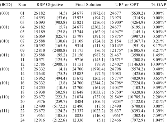
The relative di erence between the objective function value obtained by the algorithm and an upper bound or optimal solution to the originally proposed MIP model, denoted as percentage gap, and the computation time are used as performance measures in this experimental design. These performance measures will be analysed separately for two main parts of the algorithm. In the ® rst part of the algorithm, inter-cell movements are not allowed, hence the ® rst four factors are used. For this part, the results of all runs for 20 part types and 6 machine types can be seen in table 9. `RSP objective’ is the objective function value obtained by solving the relaxed subproblem, which provides an upper bound to the main problem. `Final solution’ is the objective function value obtained at the end of the second stage. The values in the parentheses are the corresponding computation times in seconds. The values in the next column of the same table, `UB* or OPT’, are the new upper bounds or the optimal solutions for the MP. If we cannot ® nd an optimum solution in a reasonable computation time then we add the following constraints klj
‡
lkjµ
1 8 k;l; j to the subproblem to obtain a tighter upper bound. Thelast column in the table is the percentage gap.
When we analyse all the results, we know the optimum solution in 10 out of 24 runs. In 5 of them, the proposed algorithm also ® nds the optimum value. In the other ® ve runs, the average gap is 0.332% with a minimum of 0.21% and a maximum of 1.45%. The average gap from the optimum value for these 10 runs is 0.116%. This means that the solution found by the algorithm is very close to the optimum value. In the other 14 runs, the optimum solution could not be found, but a new upper bound is obtained for MP. The average gap from the upper bound for these 14 runs is 5.18%. The gaps are small when we consider the di culty of solving the MP in a reasonable computation time. The average computation time is 700 seconds for the ® rst stage, 636 seconds for the second stage with a total of 1336 seconds. The constraints added to the RSP increase the computation time to an average of 5177 seconds, which is four times larger than the time needed by the proposed algorithm. Also, solving the RSP with additional constraints does not guarantee a feasible solution to the MP. But, the algorithm guarantees a feasible solution which is very close to the optimum value in all cases.
The results of the runs for 40 parts and 10 machine types can be seen in table 10. As the size of the problem increases, solving the RSP optimally in a reasonable computation time becomes more di cult. So, a predetermined time limit of 10800 seconds is used for the ® rst stage of the algorithm to ® nd a feasible integer solution for the RSP. Since this solution may not be optimal, we cannot say whether it is an upper bound for the MP or not. Also, this solution is infeasible for the MP. The objective function values of the solutions found at the end of 10 800 seconds for the ® rst stage can be seen in the third column, `RSP objective’. When the time limit is reached, the best LP relaxation value found up to that time is shown in the next column. This can be thought as an upper bound, but a loose one. The objective function values found by the RSP are smaller than the values found by the proposed algorithm, because the optimal solutions cannot be found by the RSP within the predetermined time limit. In the last column, the percentage di erence between the objective function values of the relaxed subproblem and the algorithm can be found.
This percentage shows the improvement in the objective function value. When all the results are analysed, it can be seen that a feasible solution cannot be found to any RSP in the ® rst stage. The solution found at the end of ® rst stage is improved in almost all cases by the algorithm, and the average improvement is 163%. The average computation time for the second stage is 7732 seconds. Although the com-putation times are relatively large, they are much less than the planning horizon for such a strategic level long-term planning decision.
In the second part of the algorithm, the inter-cell movements are introduced to the problem. The ® fth factor, H=h ratio, is included to the experimental design. The inter-cell movements directly increase the measurable material handling cost between cells. We know that the inter-cell moves complicate the controlling, planning and scheduling activities in a cell, but it is very di cult to estimate their intangible impact on the production cost besides the direct material handling cost. Although we only consider the measurable handling costs in our experimental design, the intangible costs can be included by relatively increasing the H=h ratio. But when this ratio is large, inter-cell moves will be undesirable compared to other alternative strategies, consequently inter-cell movement may not be allowed in order not to violate the low pro® t level constraint. The intangible costs can also be included while determining the layout of the factory by using the CRAFT algorithm by specifying di erent cost parameters for the inter-cell movements in the from-to-chart as discussed in Step 3.7. In the second part of the algorithm, we take the ® nal solution found in the ® rst part as an initial solution and try to improve it for a number of iterations. The average computation time is 362 seconds for the second part.
(BCD) Run RSP Objective Best LP Relaxation Final Solution Improvement (000) 01 9866 (10 800) 30 050 (10 800) 17 260 (1358) 75.0% 02 15 183 (10 800) 30 433 (10 800) 23 464 (3967) 54.5% 03 23 424 (10 800) 30 927 (10 800) 23 781 (1016) 1.5% (001) 04 12 771 (10 800) 28 661 (10 800) 19 153 (2125) 50.0% 05 8893 (10 800) 29 876 (10 800) 22 500 (5940) 153.0% 06 20 355 (10 800) 31 448 (10 800) 22 172 (5466) 8.9% (010) 07 2553 (10 800) 23 632 (10 800) 7262 (2039) 184.4% 08 10 784 (10 800) 24 862 (10 800) 17 439 (3448) 61.7% 09 3958 (10 800) 24 829 (10 800) 12 248 (16 063) 209.4% (011) 10 2217 (10 800) 22 997 (10 800) 10 672 (14 823) 381.4% 11 ¡2477 (10 800) 24 678 (10 800) 12 203 (3863) 592.6% 12 2202 (10 800) 25 595 (10 800) 18 127 (3019) 732.2% (100) 13 8015 (10 800) 30 558 (10 800) 16 233 (603) 102.5% 14 15 422 (10 800) 29 727 (10 800) 23 538 (13 898) 46.2% 15 26 052 (10 800) 30 970 (10 800) 25 019 (2394) ¡4:0% (101) 16 17 587 (10 800) 29 058 (10 800) 18 362 (4066) 4.4% 17 14 594 (10 800) 29 048 (10 800) 22 547 (4872) 54.5% 18 28 582 (10 800) 31 455 (10 800) 26 752 (20 674) ¡6:4% (110) 19 1656 (10 800) 24 635 (10 800) 7564 (2149) 356.8% 20 3778 (10 800) 24 205 (10 800) 17 210 (15 018) 355.5% 21 6073 (10 800) 25 077 (10 800) 13 637 (8939) 124.6% (111) 22 8159 (10 800) 23 979 (10 800) 13 162 (14 325) 61.3% 23 10 431 (10 800) 24 160 (10 800) 14 850 (708) 42.4% 24 4282 (10 800) 25 940 (10 800) 16 141 (34 806) 276.9%
Table 10. 40 parts and 10 machine types.
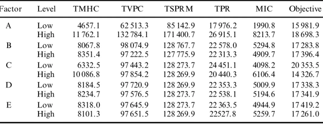
We now analyse the cost terms in the objective function and the objective func-tion value to see the individual e ect of the experimental factors on these terms. The cost terms in the objective function are total material handling cost (TMHC), total variable production cost (TVPC), di erence between total revenue and raw material cost (TSPRM), the sum of individual pro® ts of cells without considering additional machine investment cost (TPR), and the additional machine investment cost (MIC). The cost terms for each level of each factor can be seen in table 11. The values in each row are the average values of 48 runs out of 96 runs for the low and high levels of experimental design factors. The number of parts and machine types have an high e ect on all the cost terms. As the size of the system increases, total material hand-ling, production and raw material costs and revenue increases due to the high pro-duction volume. Total pro® t of cells also increases. Total additional machine investment cost increases due to either insu cient machine capacity or high material ¯ ow in cells. The increase in production cost variability does not a ect any of the performance measures signi® cantly. This may be due to the high variability in pro-cessing times of parts on machines. There is a direct relationship between material handling cost and total additional machine investment cost. When the material handling costs increase, buying new machines becomes more pro® table. Intercell material handling cost has a signi® cant impact on total material handling and addi-tional machine investment costs. When inter-cell material handling cost is low, more parts can make an inter-cell movement, which decreases the additional machine investment cost and increases the total pro® t as expected.
6. Conclusion
In this study, the part-family and machine-cell formation problems are solved with the within-cell layout problem simultaneously. The proposed approach has an advantage of allowing more accurate portrayal of the operation of CM systems by using production volumes, processing times, operation sequences and alternative routes to assess the impact of capacity constraints. To the best of our knowledge, this is the ® rst study that considers the e ciency of both individual cells and the overall system in monetary terms. Each cell should make at least a certain amount of pro® t to attain self-su ciency, while we maximize the total pro® t of the system using a holonistic approach.
An MIP model, under routing, layout, cell size, low utilization and low pro® t level constraints, is formulated to solve the PFMCF and within cell layout problems
Factor Level TMHC TVPC TSPRM TPR MIC Objective
A Low 4657.1 62 513.3 85 142.9 17 976.2 1990.8 15 981.9 High 11 762.1 132 784.1 171 400.7 26 915.1 8213.7 18 698.3 B Low 8067.8 98 074.9 128 767.7 22 578.0 5294.8 17 283.8 High 8351.4 97 222.5 127 775.9 22 313.3 4909.7 17 396.4 C Low 6332.5 97 443.2 128 273.7 24 451.1 4098.2 20 353.5 High 10 086.8 97 854.2 128 269.9 20 440.3 6106.4 14 326.7 D Low 8184.5 97 720.9 128 269.9 22 353.3 5009.9 17 338.3 High 8234.7 97 576.5 128 273.7 22 538.1 5194.6 17 341.9 E Low 8318.0 97 645.9 128 273.7 22 363.5 4944.9 17 419.2 High 8101.3 97 651.5 128 269.9 22527. 8 5259.7 17 261.0
Table 11. Average cost values for low and high level of each factor.
simultaneously to maximize the total pro® t. We also propose a local search algor-ithm, which provides two alternative solutions; one with independent cells and the other one with inter-cell movement. The results of the experimental design are very encouraging. The proposed algorithm always ® nds a feasible solution to the problem in a reasonable computation time. When the size of the problem is small, the average gap is only 0.116% for the 20 part and 6 machine type problems for which we know the optimum values. The computation times of the algorithm are signi® cantly less than the computation times needed to ® nd tight upper bounds to the main problem. When the problem size increases, a tight upper bound cannot be found for compar-ison purposes. But, the objective function value obtained at the end of ® rst stage is improved signi® cantly with an average of 163%. Since this problem is a strategic level long-term design problem, the run times are much less than the planning horizon.
References
ADIL
,
G.
K.,
RAJAMANI,
D.
and STRONG,
D.
, 1996, Cell formation considering alternate routings. International Journal of Production Research, 34, 1361-1380.AKTURK
,
M.
S.
andBALKOSE,
H.
O.
, 1996, Part machine grouping using a multi-objective cluster analysis. International Journal of Production Research, 34, 2299± 2315.ASKIN
,
R.
andZHOU,
M.
, 1998, Formation of independent ¯ ow-line cells based on operation requirements and machine capabilities. IIE T ransactions, 30, 319± 329.BAZARGAN
-
LARI,
M.
and KAEBERNICK,
H.
, 1996, Intracell and intercell layout designs for cellular manufacturing. International Journal of Industrial Engineering, 3, 139± 150. BEAULIEU,
A.,
GHARBI,
A.
and AIT-
KADI,
D.
, 1997, An algorithm for cell formation andmachine selection problems in the design of a cellular manufacturing system.
International Journal of Production Research, 35, 1857± 1874.
CHOOBINEH
,
F.
, 1988, A framework for the design of cellular manufacturing systems.International Journal of Production Research, 26, 1161± 1172.
DAHEL
,
N.
E.
, 1995, Design of cellular manufacturing system in tandem con® guration.International Journal of Production Research, 33, 2079± 2095.
HERAGU
,
S.
S.
and GUPTA,
Y.
P.
, 1984, A heuristic for designing cellular manufacturing facilities. International Journal of Production Research, 32, 125± 140.HO
,
Y.
C.
and MOODIE,
C.
L.
, 1996, Solving cell formation problems in a manufacturing environment with ¯ exible processing and routing capabilities. International Journal ofProduction Research, 34, 2901± 2923.
HO
ï
PF,
M.
, 1994, Holonic manufacturing systems. CIM-Europe Annual Conference, Copenhagen, pp. 84± 93.JOINES
,
J.
A.,
CULBRETH,
C.
T.
andKING,
R.
E.
, 1996, Manufacturing cell design: an integer programming model employing genetic algorithms. IIE Transactions, 28, 69± 85. OFFODILE,
O.
F.,
MEHREZ,
A.
andGRZNAR,
J.
, 1994, Cellular manufacturing: A taxonomicreview framework. Journal of Manufacturing Systems, 13, 196± 219.
VAKHARIA
,
A.
J.
andCHANG,
Y.-
L.
, 1997, Cell formation in group technology: A combina-torial search approach. International Journal of Production Research, 35, 2025± 2043. VAKHARIA,
A.
J.
and WEMMERLOï
V,
U.
, 1990, Designing a cellular manufacturing system: Amaterials ¯ ow approach based on operation sequences. IIE T ransactions, 22, 84± 97. VERMA
,
P.
andDING,
F.-
Y.
, 1995, A Sequence-based materials ¯ ow procedure for designingmanufacturing cells. International Journal of Production Research, 33, 3267± 3281.