Classification of vessel acoustic signatures using non-linear scattering based feature extraction

CLASSIFICATION OF VESSEL ACOUSTIC

SIGNATURES USING NON-LINEAR

SCATTERING BASED FEATURE

EXTRACTION

a thesis submitted to

the graduate school of engineering and science

of bilkent university

in partial fulfillment of the requirements for

the degree of

master of science

in

electrical and electronics engineering

By

G¨

okmen Can

September 2016

CLASSIFICATION OF VESSEL ACOUSTIC SIGNATURES USING NON-LINEAR SCATTERING BASED FEATURE EXTRACTION By G¨okmen Can

September 2016

We certify that we have read this thesis and that in our opinion it is fully adequate, in scope and in quality, as a thesis for the degree of Master of Science.

A. Enis C¸ etin(Advisor)

Hitay ¨Ozbay

Kasım Ta¸sdemir

Approved for the Graduate School of Engineering and Science:

Levent Onural

ABSTRACT

CLASSIFICATION OF VESSEL ACOUSTIC

SIGNATURES USING NON-LINEAR SCATTERING

BASED FEATURE EXTRACTION

G¨okmen Can

M.S. in Electrical and Electronics Engineering Advisor: A. Enis C¸ etin

September 2016

This thesis proposes a vessel recognition and classification system based on acous-tic signatures. Conventionally, acousacous-tic sounds are recognized by sonar operators who listen to audio signals received by ship sonars. The aim of this work is to replace this conventional human-based recognition system with an automatic feature-based classification system. Therefore, it can be regarded reasonable to adopt the speech recognition algorithms in classification of underwater acoustic signal recognition (UASR). The most widely used feature extraction methods of speech recognition are Linear Predictive Coding (LPC) and Mel Frequency Cepstral Coefficients (MFCC) and they are also used in UASR. In addition, the Scattering transform is used to obtain filter bank instead of mel-scale filter bank in MFCC algorithm. The scattering cascade decomposes an input signal into its wavelet modulus coefficients and various non-linearities are used between wavelet stages. The new proposed method is labeled as Scattering Transform Cepstral Coefficients (STCC). Sensitivity of human hearing system is not the same in all frequency bands and mel-scale filter bank in MFCC is more sensitive to small changes in low frequencies than high frequencies. Therefore, number of DWT decomposition levels is increased in low frequencies to determine accurate repre-sentation and experimental results shows that non-uniform filter banks provide better success rates. Non-linear Teager energy and hyperbolic tangent operators are used to increase the performance of classification in proposed features ex-traction methods. Non-linear operators and scattering transforms are used for the first time in UASR to identify the acoustic sounds of the platforms. Teager Energy Operator (TEO) estimates the true energy of the source of a resonance signal. TEO based MFCC, being more robust in noisy conditions than conven-tional MFCC, provides a better estimation of the platform energy. Although

iv

TEO has positive effect on MFCC, it decreases the performance of STCC. Differ-ent non-linear tanh operator is also applied to LPC, MFCC and STCC algorithms and experimental results show that tanh operator increases the performance of the classification in all feature extraction methods. This analysis and implemen-tation was carried out with datasets of 24 different vessel signals recordings that belong to 10 separate classes of vessels. Artificial Neural Networks (ANN) and Support Vector Machines (SVM) are used as classifiers. Performance of the pro-posed methods is compared and experimental results demonstrate that STCC have the best performance and tanh based STCC achieves highest success rate with 98.50% accuracy in classification of vessel sounds.

Keywords: Vessel Recognition, LPC, MFCC, Wavelet Filter Bank, Teager Energy Operator, Scattering Transform.

¨

OZET

DO ˘

GRUSAL OLMAYAN SAC

¸ ILMA TEMELL˙I

¨

OZN˙ITEL˙IK C

¸ IKARMA KULLANARAK GEM˙ILER˙IN

AKUST˙IK ˙IZLER˙IN˙IN SINIFLANDIRILMASI

G¨okmen Can

Elektrik Elektronik M¨uhendisli˘gi, Y¨uksek Lisans Tez Danı¸smanı: A. Enis C¸ etin

Eyl¨ul 2016

Bu tez gemilerin akustik izlerine dayanan gemi tanıma ve sınıflandırma sistemi ¨

onermektedir. Sonar operat¨orlerin, gemi sonarları tarafından algılanan akustik sesleri dinleyerek geleneksel y¨ontemlerle tanıma yapmaktadır. Bu ¸calı¸smanın amacı, insana dayanan tanıma sistemini otomatik bilgisayar tabanlı sınıflandırma sistemi ile de˘gi¸stirmektir. Bundan dolayı, konu¸sma tanıma algoritmalarındaki ¨

oznitelik vekt¨orleri sualtı akustik sinyallerin tanınmasında da (UASR) kabul et-mek mantıklı bir d¨u¸s¨unce olacaktır. Konu¸sma tanımada en yaygın kullanılan ¨

oznitelik vekt¨or ¸cıkarma algoritmaları Do˘grusal Kestirimci Kodlama (LPC) ve Mel Frekans Kepstral katsayılarıdır (MFCC) ve ayrıca bu iki metot UASR’de de kullanılmı¸stır. Ek olarak, s¨uzge¸c bankasını elde etmek i¸cin MFCC algo-ritmasında bulunan mel ¨ol¸cekli s¨uzge¸c bankası yerine Sa¸cılma d¨on¨u¸s¨um¨u kul-lanılmı¸stır. Sa¸cılma, sinyali ardı ardına aralarında do˘grusal olmayan operat¨orlerin bulundu˘gu dalgacık d¨on¨u¸s¨umleriyle b¨olm¨u¸s ve dalgacık katsayılarını elde etmi¸stir.

¨

Onerilen yeni metod Sa¸cılma D¨on¨u¸s¨um¨u Kepstral katsayıları (STCC) olarak isimlendirilmi¸stir. ˙Insanın duyma hassasiyeti b¨ut¨un frekans bantlarında aynı de˘gildir ve MFCC d¨u¸s¨uk frekanslardaki de˘gi¸simlere y¨uksek frekansa g¨ore daha hassastır. Bu nedenle daha do˘gru bir g¨osterim yapabilmek i¸cin d¨u¸s¨uk frekanslarda DWT sayını arttırarak daha ¸cok b¨ol¨unme i¸slemi yapılmı¸stır ve deneysel sonu¸clar g¨ostermi¸stir ki e¸sda˘gılım yapmayan s¨uzge¸c bankası daha iyi ba¸sarı g¨ostermi¸stir.

¨

Onerilen ¨oznitelik ¸cıkarma metodlarında sınıflandırma performansını arttırmak i¸cin farklı do˘grusal olmayan operat¨orler kullanılmı¸stır. Do˘grusal olmayan op-erat¨orler ve sa¸cılma d¨on¨u¸s¨um¨un¨un uygulanması akustik g¨ur¨ult¨u ¨ureten platform-ları tanımada ilk kez kullanılacaktır. Teager enerji operat¨or¨u (TEO) bulunan MFCC’nin g¨ur¨ult¨ul¨u ortamlara daha dayanıklı oldu˘gu ve platformların enerji-lerinin daha iyi tahmin edilmesini sa˘gladı˘gı g¨or¨ulm¨u¸st¨ur. TEO’nun MFCC’de

vi

positif etkisi olmasına ra˘gmen STCC’de performansı d¨u¸s¨urm¨u¸st¨ur. Ayrıca farklı bir do˘grusal olmayan tanh operat¨or¨u LPC, MFCC ve STCC’ye uygulanmı¸s ve deneysel sonu¸clar bu operat¨or¨un b¨ut¨un ¨oznitelik ¸cıkarma metodlarında perfor-mansı arttırdı˘gı g¨osterilmi¸stir. Analiz ve uygulama 10 farklı sınıfa ait 24 farklı gemi sesi kaydının oldu˘gu veri k¨umesi ile y¨ur¨ut¨ulm¨u¸st¨ur. Sınıflandırıcı olarak Ya-pay Sinir A˘gı (YSA) ve Destek¸ci Vekt¨or Makinası (DVM) kullanılmı¸stır. ¨Onerilen metotların performansları kar¸sıla¸stırılmı¸stır ve deneysel sonu¸clar STCC’nin en iyi sınıflandırma performansına sahip oldu˘gu kanıtlanmı¸stır ve tanh uygulanan STCC’nin gemi seslerini sınıflandırmada %98,50 do˘gruluk ile en y¨uksek oranı ba¸sarmı¸stır.

Anahtar s¨ozc¨ukler : Gemi Tanıma, LPC, MFCC, Wavelet s¨uzge¸c Bankası, Teager Energy Operat¨or¨u.

Acknowledgement

My first and foremost thanks goes to my mother, my brothers, my wife Nihan for taking care of our daugter during the most difficult times of thesis writing, and my daugter Defne who is new member of my family. None of this would have happened without them and I am deeply indebted for their continuous and unconditional support. Besides all, they also took major parts in my life-long learning process:

I would also like to express my deepest gratitude to:

• My thesis advisor Dr. Ahmet Enis C¸ etin for sharing his invaluable academic and life experiences with me.

• My thesis committee members Dr.Hitay ¨Ozbay and Dr. Kasım Ta¸sdemir for their valuable feedback.

• ASELSAN for providing dataset of Vessel Signals .

• Cem Emre Akba¸s, Emre Top¸cu and Erdal Mehmet¸cik for sharing his pre-cious research experience with me and for his contributions to my research. • My maneger Deniz Durusu for tolerance.

Contents

1 Introduction 1

2 Background Information and Experiment 5

2.1 Linear Predictive Coding (LPC) . . . 5

2.2 Mel-Frequency Cepstral Coefficients (MFCC) . . . 10

2.2.1 Pre-emphasis Block . . . 11

2.2.2 Framing Block . . . 11

2.2.3 Windowing Block . . . 12

2.2.4 Mel-Filter Bank . . . 12

2.2.5 Logarithm Operation . . . 16

2.2.6 Discrete Cosine Transform Block (DCT) . . . 16

2.3 Teager Energy Operator (TEO) . . . 18

2.4 Discrete Wavelet Transform . . . 19

CONTENTS ix

2.6 Classification Algorithms . . . 25

2.6.1 Artificial Neural Networks (NN) . . . 25

2.6.2 Support Vector Machines (SVM) . . . 26

2.7 Results . . . 27

2.7.1 LPC Classification Results . . . 27

2.7.2 MFCC Classification Results . . . 29

3 Teager Energy and Hyperbolic Tangent Operators based Fea-tures of Existing Methods 32 3.1 Tanh Operator based LPC Features . . . 32

3.2 TEO based LPC Features . . . 33

3.3 TEO based MFCC Feature Parameters . . . 33

3.3.1 Classification using t-TEO MFCC . . . 33

3.3.2 Classification using TEO MFCC . . . 34

3.4 Tanh Operator based MFCC Feature Parameters . . . 35

3.5 Results . . . 35

4 Scattering Transform Based Feature Extraction 40 4.1 Scattering Transform Cepstral Coefficients (STCC) Features . . . 40

4.2 Tanh Operator based STCC Feature Parameters . . . 43

CONTENTS x

4.4 STCC Based on Non-uniform Filterbank . . . 48

4.5 Comparision of Classification Results . . . 51

List of Figures

1.1 Main components of the classification system [1]. . . 2

2.1 Linear Prediction System . . . 7

2.2 LPC Spectrum of Vessel-A 5knot . . . 8

2.3 LPC Spectrum of Vessel-B 5knot . . . 9

2.4 LPC Spectrum of Vessel-C 6knot . . . 9

2.5 Block Diagram of MFCC . . . 10

2.6 Framing Structure . . . 11

2.7 Effect of the Hamming Windowing [2] . . . 12

2.8 Linear vs Mel-scaling . . . 14

2.9 Triangular mel-scale filter bank . . . 15

2.10 Mel-filter bank processing . . . 15

2.11 Type-A 5knot Filterbank Energy and MFCC . . . 17

LIST OF FIGURES xii

2.13 Type-B 10knot Filterbank Energy and MFCC . . . 18

2.14 Block Diagram of 1-Level DWT . . . 21

2.15 Map of Experiment and Position of Vessels . . . 22

2.16 Vessel Type-A . . . 24

2.17 Vessel Type-B . . . 24

2.18 Two Layer Feed-Forward Network . . . 25

2.19 Distribution of Training Data in NN . . . 25

2.20 Concept Example of SVM . . . 26

2.21 Curve Separation for SVM . . . 27

2.22 Kernels Mapping for SVM . . . 27

2.23 LPC Success Rates . . . 28

2.24 Performance of MFCC According to Various # of Channels . . . . 30

3.1 Applying Tanh Operator to LPC Process . . . 32

3.2 Applying TEO to LPC Process . . . 33

3.3 Block Diagram of t-TEO MFCC . . . 33

3.4 Block Diagram of TEO MFCC . . . 34

3.5 Applying Tanh Operator to MFCC Process . . . 35

3.6 Comparison of MFCC and TEO-MFCC Performances . . . 37

LIST OF FIGURES xiii

3.8 Comparison of Classification Methods in TEO based MFCC Features 39

4.1 The Block Diagram of the STCC Algorithm . . . 41

4.2 The filter bank without nonlinear scattering . . . 42

4.3 Scattering filter bank using the nonlinearity tanh(x[n]₅ ) function . . 44 4.4 Comparison of STCC and Tanh-STCC Performances . . . 46

4.5 Scattering filter bank using the nonlinear TEO . . . 47

4.6 Comparison of WTCC and TEO-STCC Feature extraction schemes 48

4.7 Non-uniform filter bank without nonlinear scattering . . . 49

4.8 Non-uniform Scattering filter bank using the nonlinearity tanh(x[n]₅ ) function . . . 50

List of Tables

2.1 Vessel Database and Description . . . 23

2.2 LPC Classification Success Rates . . . 28

2.3 NN classification success rates of MFCC . . . 29

2.4 Performance of MFCC according to various # of channels . . . . 30

3.1 Tanh and TEO based LPC results . . . 36

3.2 MFCC and TEO based MFCC classification rates . . . 36

3.3 Results of various classification methods in MFCC features . . . . 38

3.4 TEO and Tanh based MFCC results . . . 39

4.1 Tanh based STCC results . . . 45

4.2 TEO based STCC results . . . 47

4.3 STCC success rates using tanh op. in a non-uniform filter bank . 51

Chapter 1

Introduction

Detection, classification and tracking of vessels are very significant for underwater surveillance system and improving coast and off-shore security. Passive underwa-ter acoustic sensors are used to detect vessels noise and gather data. Vessel noise is an acoustic signature and it can be used for vessel detection and classification.

Underwater acoustic signal detection methods are based on sounds produced by moving vessels. The main sources of vessel noise are propellers and engine mechanisms (blades, rotation and propeller radiated pressure). Passive acoustic methods have been used in submarines for years, and they were published after World War II [3] [4]. There is also environmental noise such as the noise generated by waves, wind, rainfall, etc.

Every person has a unique voice and the characteristic of this voice is used for speaker identification in speech recognition. Similarly, every ship also has a different noise source combination (number of blades, rotational speed and pro-peller radiated pressure etc.).This combination creates a unique signature sound for every vessel. This uniqueness can be considered as an acoustic signature for vessels. As a result, automatic speaker recognition (ASR) and classification al-gorithms developed in speech recognition can be used for Underwater Acoustic

Signal Recognition (UASR) to identify platforms based on their acoustic signa-tures.

At the top level, there are two main modules which are feature extraction and feature matching in all signal classification systems. First step feature extraction is a process which extracts a small amount of data from acoustic signatures. These feature extractions will be used for representation of each object. Second step is a feature matching process which identity the unknown objects feature parameters from input sound using the set of known extracted features in database. Main parts of acoustic signatures classification system is basically given in Figure 1.1 [1].

Figure 1.1: Main components of the classification system [1].

Feature extraction is the most important and difficult part for classification. Because feature extraction process will be unique for a given source of sound or acoustic signature and this process will not change independently with exter-nal noise. Also, for successful classification, classification system should not be complex and operate real time. Therefore, feature extraction part is the most essential part of the quality of the success.

Conventionally, classification of vessel signatures is carried out by an experi-enced submarine sonar operator who listens to the acoustic noise coming from the ship sonars. It is evident that it would be more feasible to develop a computer based vessel signature recognition system using ASR methods. Therefore, widely

used speech recognition methods are used for feature extraction in our work and it is shown that these methods can be easily be adapted to classification of vessel noise with good success rate [5].

Different Speech Recognition methods are used for extraction feature vectors in UASR and this article starts to examine Linear Predictive Coding (LPC) method for features. LPC is a signal source modeling method and most widely used in speech and speaker recognition. LPC method estimates extremely accurate spectral envelope and different speech parameters.

This thesis continues with a second method for classification of ship signatures which extracts feature vector using Mel Frequency Cepstral Coefficients (MFCC) frame by frame. It is widely used in speech recognition systems and produces good results on speech recognition and identification.

This thesis offers a modified version of MFCC that utilizes TEO for classi-fication of vessel signatures. Applying non-linear Teager energy operator can suppress environmental noise and increase the classification performance [6, 7]. TEO is used in various speech recognition applications, but it will be used for the first time in UASR and a good candidate for proposed feature parameters in vessel signatures. The proposed features are evaluated to show that TEO-MFCC is more robust than MFCC and LPC with higher classification success rate.

This thesis continues with a third novel method. MFCC feature vectors are extracted using wavelet transform instead of the mel-scale filter bank and Fast Fourier Transform. In conventionally MFCC; magnitude spectrum of windowed frames are calculated, than mel-scale triangular filter bank is applied to magni-tude spectrum to obtain energies of each filter bank. However in this method, energies of filterbank are obtained using Scattering Transform which is consist of cascading DWT and non-linear modules. Signal component are estimated in different frequency bands using DWT and energies are obtained from DWT coefficients. Windowing, logarithm and DCT blocks are the same with MFCC algorithm. Cepstral coefficients based on scattering transform will be labeled as Scattering Transform Cepstral Coefficients (STCC).

STCC already depends on non-linear operators in filter bank, but different non-linear operator tan(x[n]/a) where a is the positive number greater than 1, is also applied to LPC and MFCC algorithms to increase the performance of the classification success rates.

Classification of feature vectors problem is analysed by two methods. First classification method is Neural Pattern Recognition Application in Matlab Neural Network toolbox [8]. Application classifies features into a set of target categories using a two layer feed-forward network. Network structure has one hidden layer and one output layer. These layers are trained to classify test data according to target classes. Second classification method is support vector machines (SVMs) in Matlab Classification Learner Application. This application performs supervised machine learning by supplying a known set of input data (observations) and known responses to the data (classes). Various classifiers can be used in this application, linear and quadratic SVMs are selected in our thesis.

Chapter 2

Background Information and

Experiment

In this chapter, we review the existing methods for classification of vessel sounds. Current methods include;

• Linear Predictive Coding (LPC),

• Mel-Frequency Cepstral Coefficients (MFFC), and

• Discrete Wavelet Transform based feature extraction methods.

2.1

Linear Predictive Coding (LPC)

LPC method is extensively used in speech coding, speech recognition, speaker recognition and verification. LPC is an encoding method using linear prediction model. Basic idea of linear prediction model is that, trying to predict next point as linear combination of previous values [1].

x(n) =

P

X

k=1

akx(n − k) + e(n), (2.1)

where x(n − k) are past or previous signal samples, ak is prediction coefficient, P

is model order, and e(n) is error of prediction.

The prediction signal ˆx(n) can be written as follows:

ˆ x(n) = P X k=1 akx(n − k) (2.2)

Application of this method is for compressing a signal by coding residual or er-ror signal. Residual signal is difference between original and predicted (estimated) signals. Predictor coefficients (ak’s) can be computed by several methods. Our

coefficients are determined by minimizing the sum of squared differences between the actual signal samples and linearly predicted signal samples.

Pth _{order linear prediction system form can be written as follows:}

P (z) = ˆ X(z) X(z) = P X k=1 akz−k (2.3)

The prediction error signal e(n) can be written as follows:

e(n) = x(n) − ˆx(n) = x(n) −

P

X

k=1

akx(n − k) (2.4)

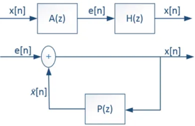
The transfer function of the prediction error system’s A(z) can be expressed as follows: A(z) = E(z) X(z) = 1 − P (z) = 1 − P X k=1 akz−k (2.5)

And, H(z) is the inverse filter of A(z):

H(z) = 1

Figure 2.1: Linear Prediction System

We need to determine the predictor coefficients ak to minimize mean-squared

prediction error over short segment of signal. Shortly, end of the minimizing mean-squared prediction error, autocorrelation matrix will be obtained and solved with Levinson-Durbin algorithm to find predictor coefficients [10].

LPC represents the spectral envelope of signal using linear predictive model and it is used for transmitting envelope information. Impulse response of the LPC-systems transfer function gives the envelope information and LPC order arranges the quality of the envelope. Spectral envelopes of vessel types are plotted with various LPC order to show differences. Performance of various orders will be given to compare classification success rates.

0 1000 2000 3000 4000 5000 6000 7000 8000 9000 10000 frequency (Hz) -120 -100 -80 -60 -40 -20 0 PSD (dB)

Type A 5 knot/1 3 Seconds Records Power Spectrum 10-Order LPC 20-Order LPC 30-Order LPC 40-Order LPC

Figure 2.2: LPC Spectrum of Vessel-A 5knot

When LPC order increases, the algorithm produces a better spectral envelope. It is obviously shown that 30 and 40 orders are enough to provide good spectral envelope as shown in Figure 2.2 2.3 and 2.4.

0 1000 2000 3000 4000 5000 6000 7000 8000 9000 10000 frequency (Hz) -140 -120 -100 -80 -60 -40 -20 PSD (dB)

Type B 5 knot/1 3 Seconds Records

Power Spectrum 10-Order LPC 20-Order LPC 30-Order LPC 40-Order LPC

Figure 2.3: LPC Spectrum of Vessel-B 5knot

0 1000 2000 3000 4000 5000 6000 7000 8000 9000 10000 frequency (Hz) -120 -110 -100 -90 -80 -70 -60 -50 -40 -30 -20 PSD (dB)

Type C 6 knot 3 Seconds Records

Power Spectrum 10-Order LPC 20-Order LPC 30-Order LPC 40-Order LPC

These three examples are enough to understand the effect of the LPC spectrum envelope. LPC orders are plotted disjoint to see differences. Peaks and format points are estimated well in type-A vessel spectrum. However, type-B and type-C spectrum envelopes are not estimated well as type-A. This may be due to reason that peaks are very close to each other and environment is not clear as type-A environment. LPC coefficients are no longer used in speech recognition. The most widely used method is MFCC, which will be covered in the next section.

2.2

Mel-Frequency Cepstral Coefficients (MFCC)

Sound is generated in humans by vocal cords and the shape of the vocal tract (tongue, teeth etc.) filters this sound. This shape or filtering determines what sound comes out. If shape is determined accurately, an accurate representation of the produced phoneme can be obtained. This shape appears in the envelope of the power spectrum of the generated sound. Since the shape of the vocal tract can be represented by MFCC accurately, this method is widely used in ASR [11]. We expect that MFCC also can represent vessel sounds accurately.

The block diagram of the MFCC algorithm is given in Figure 2.5. Each block is explained in the following subsections.

2.2.1

Pre-emphasis Block

This step is the filtering of the vessel acoustic noise by the filter defined in Equa-tion 2.7.

y[n] = x[n] − 0.95x[n − 1] (2.7)

This filter boosts higher frequencies so that after filtering, the energy of the signal increases at higher frequencies. The noise signal has smaller amplitudes at high frequency components with respect to low frequencies. After this block, high frequency components of the signal become more significant and more information about the acoustic model is obtained [12].

2.2.2

Framing Block

The importance of this block is that much shorter frames have unreliable spectral estimate and longer frames change too much. Although speech signal is non-stationary, short time scales will be stationary. The reason for this is that the width of the frames is chosen as 25ms with 10ms overlap. In this case frames are 15ms shifted.

2.2.3

Windowing Block

Windowing functions are used before computing the Fourier transform.

In this thesis, Hamming window is used for this purpose:

Figure 2.7: Effect of the Hamming Windowing [2]

w[n] = (

0.54 − 0.46cos(_{N −1}2πn), 0 ≤ n ≤ N − 1

0, otherwise (2.8)

In Figure 2.7 a sound waveform block and its windowed version are shown.

2.2.4

Mel-Filter Bank

2.2.4.1 Mel Scale

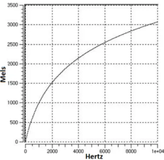
Sensitivity of human hearing system is not the same in all frequency bands. Mel (melody) is a unit of measure based on human ears perceived frequency. Human ear’s are less sensitive at higher frequencies, and more sensitive to small variations

in low frequencies compared to high frequencies. Mel-scaling based frequency warping makes our features closer to what humans hear. 1 kHz is defined as 1000 mels as a reference [13].

Warping expression from linear-scale to mel-scale in frequency domain is given by: M el(f ) = 2595 × log10(1 + f 700), (2.9) or M el(f ) = 1125 × ln(1 + f 700) (2.10)

Converting formula from mel-scale to linear-scale is given by:

M el−1(m) = 700 × e1125m −1. (2.11)

Below 1 kHz, mel-scaling is similar to linear frequency spacing. Above 1 kHz, it is more logarithmic as shown in Figure 2.8 [14].

Figure 2.8: Linear vs Mel-scaling

2.2.4.2 Mel Filterbank

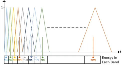
Mel filterbank is implemented as follows:

• Decide on the lower and upper frequencies of the filterbank based on the sampling frequency, and convert to limits from frequency to mels.

• Decide the number of filters. (n+2) frequency values are needed for n filters. These mel values are linearly spaced between the limits in mel domain. • Convert these (n + 2) mel points into frequency domain.

• Based on the FFT size and sampling rate, it is required to convert the frequencies into FFT bin numbers. Exact values in frequency domain should be rounded to the nearest FFT bins and this process does not affect the accuracy.

• First filter start with first point, maximize at second point and return the zero again at third point [11].

In Figure 2.9, triangular windows are uniformly spaced according to the mel-scale.

Figure 2.9: Triangular mel-scale filter bank

Filterbank has not equal gain distribution, because filters have different fre-quency widths. But it is experimentally observed that it does not matter in speech recognition [15].

After calculating mel-scale filter bank in frequency domain, we apply them to the spectrum of the signal. The Figure 2.10 summarizes this operation:

Last step of the mel-filter bank is to calculate the energies of the filter bank outputs. Multiplying each filter bank by the magnitude spectrum of the signal and then adding up the coefficients yields how much energy there is in each filter region. In Figure 2.10, Y(m) is the energy at the output of the m-th filter and M is the number of filters.

2.2.5

Logarithm Operation

The human perception of sound intensity approximates the logarithmic scale rather than linear. This means that, humans are less sensitive to small changes at high amplitudes than low amplitudes. That is why logarithm of Y(m) are computed before computing the DCT.

2.2.6

Discrete Cosine Transform Block (DCT)

This block converts logarithmic mel-spectrum into quefrequency domain and the result is labeled as Mel Frequency Cepstral Coefficients (MFCC):

y[k] = M X m=1 log(|Y (m)|)cos(k(m − 0.5) π M) k = 0, 1, ...M − 1 (2.12)

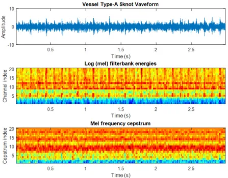
We need to show that MFCC values should be independent of the speed of a given vessel and distribution is similar regardless of the speed of the vessel. However, different types of vessels with the same velocity should have different MFCC values, otherwise we cannot use values as feature vectors of vessel sounds.

The following Figures 2.11, 2.12 and 2.13 show MFCC distribution and filter-bank energies. Although Type-B 5 knot and 10 knot have similarity, Type-B and Type-A 5 knots have different distributions.

Figure 2.11: Type-A 5knot Filterbank Energy and MFCC

Figure 2.13: Type-B 10knot Filterbank Energy and MFCC

2.3

Teager Energy Operator (TEO)

TEO is an energy operator and it can eliminate the effect of noise in feature extraction. It provides a good estimation of the real source of energy and ensures that the system will be more robust in noisy environments. For clean conditions, the system performs similarly [16].

Teager Energy Operator is defined for real continuous-time signals in the fol-lowing equation:

Ψ(x(t)) = ˙x(t)2− x(t)¨x(t) (2.13) ,and for real discrete-time signals can be written as follows:

The case of complex continuous-time signals, the equation is given as:

Φ(x(t)) = Ψ(Real{x(t)}) + Ψ(Im{x(t)}), (2.15) and for discrete-time:

Φ(x[n]) = Ψ(Real{x[n]}) + Ψ(Im{x[n]}) (2.16)

2.4

Discrete Wavelet Transform

Wavelet transform is the decomposition of a signal with orthonormal basis ψm,n(x). It is known as the mother wavelet and, signal is obtained through

translation and dilation of the basis functions. Fourier transform is used sines and cosines function for basis, but wavelets transform is represented by different types of basis functions. Fourier basis are localized in only frequency domain, not in time. Small frequency changes in the Fourier transform will affect everywhere in the time domain but wavelets are local in both frequency (because of dila-tions) and time (because of transladila-tions) domain. This is a advantage of wavelet transform.

ψm,n(x) = 2−m/2ψ(2−mx − n) (2.17)

where m and n are integers. The wavelet coefficients of a signal f(x), can be written as follows because of the orthogonality property;

cm,n =

Z +∞

−∞

f (x)ψm,n(x)dx (2.18)

f (x) =X

m,n

cm,nψm,n(x) (2.19)

Before construction of mother wavelet, scaling function φ(x) should be deter-mined with satisfying following two equations;

φ(x) =√2X k h(k)φ(2x − k) (2.20) and, ψ(x) =√2X k g(k)φ(2x − k) (2.21) where g(k) = (−1)kh(1 − k) (2.22) The coefficients of h(k) given in Equation 2.20 need to satisfy some conditions. Set of basis wavelet functions must be unique, orthonormal, and have a certain degree of regularity. There are a lot of sets of coefficients h(k) satisfying the above conditions in literature like Haar, Daubechies, Fejer-Korovkin, Lagrange etc. wavelet filters [17, 18, 19, 20, 21].

The coefficients h(k) and g(k) play a very crucial in discrete wavelet transform because φ(x) and ψ(x) are only depends on h(k).

The procedure starts with passing this signal (sequence) through a half-band digital lowpass filter with impulse response h[n].

The DWT coefficients of a input signal is obtained by passing through a series of filters. The procedure starts with passing the input signal through a half band digital lowpass filter with impulse response h[n] and highpass filter with impulse response g[n] simultaneously. Half of the samples will be eliminated according to the Nyquist’s rule, and maximum frequency of signal will be π/2 radians instead of π. Therefore, signal is downsampling by 2 to eliminate half of the samples.

Figure 2.14: Block Diagram of 1-Level DWT

Mallat’s common notation is as follows:

ylow[n] =

X

n

x[n]h[2k − n], (2.23)

where ylow[n] are the approximation coefficients and the detail coefficients are:

yhigh[n] =

X

n

x[n]g[2k − n] (2.24)

In this thesis, a multilevel DWT filter bank is used to obtained wavelet coeffi-cients and details are given in Chapter-4.

2.5

Experiments

The data sets containing the records of 19 acoustic signatures from 6 types of vessels were provided by ASELSAN. The acoustic signatures were recorded by an acoustic sensor submerged underwater from a stationary vessel while another vessel moves and produce noise (its acoustic signature). The moving vessel ap-proaches and moves away from the stationary sensor at different velocities and records are taken at varying distances. The distance between the moving and sta-tionary vessels is measured both by GPS and laser rangefinder and this distance is synchronized with the acoustic recordings.

Figure 2.15: Map of Experiment and Position of Vessels

On the stationary vessel, Reson TC4032 hydrophone is used as the acoustic sensor. Data acquisition is performed at 100 kHz or 200 kHz sampling rate. Records are decimated by a factor of 5 or 10 to provide 20 kHz sampling rate and also divided into smaller frames in order to be treated as a short record of the underwater acoustic signatures.

In addition to records provided by ASELSAN, records found on National Park Service (NPS) open-internet source were used in the experiments in order to get more realistic experimental results. However in these open-source records; distance between sensor and vessel and velocity are generally unknown. Different classes of vessels were chosen (ferry, freighter, cruise ship, and outboard) with respect to previous vessels to increase database.

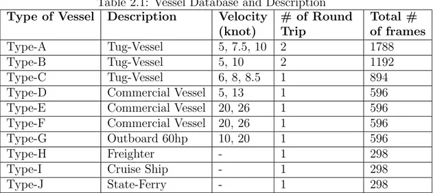
Table 2.1: Vessel Database and Description

Type of Vessel Description Velocity # of Round Total # (knot) Trip of frames Type-A Tug-Vessel 5, 7.5, 10 2 1788

Type-B Tug-Vessel 5, 10 2 1192

Type-C Tug-Vessel 6, 8, 8.5 1 894 Type-D Commercial Vessel 5, 13 1 596 Type-E Commercial Vessel 20, 26 1 596 Type-F Commercial Vessel 20, 26 1 596 Type-G Outboard 60hp 10, 20 1 596

Type-H Freighter - 1 298

Type-I Cruise Ship - 1 298

Type-J State-Ferry - 1 298

and duration of each record in the database is 3 seconds long. 3 seconds records are divided into 25 ms frames with 10ms overlap. Our proposed method is tested with various velocities of vessels between 5 knots and 26 knots. Table-1 shows acoustic noise of platforms, their velocities and number of frames. The records of Tug-vessels and commercial vessels (Type A-F) were provided by ASELSAN as explained in previous chapter, other records were found on NPS open internet source and only the velocity of outboard is known [22].

Figure 2.16: Vessel Type-A

2.6

Classification Algorithms

2.6.1

Artificial Neural Networks (NN)

Classification of feature vectors problem is solved by Neural Pattern Recognition Application in Matlab Neural Network toolbox. Application classifies features into a set of target categories using a two layer feed-forward network. Network structure has one hidden layer and one output layer.

Figure 2.18: Two Layer Feed-Forward Network

The length of input is equal to the length of the feature vector, the number of output layer neurons is equal to the number of target classes and the number of hidden layer neurons is chosen as 10. The target data should consist of vectors of all zero values except for a 1 in element i, where i is the class they are to present. Therefore, application is supervised learning and it updates the weights according to the scaled conjugate gradient backpropagation method [8].

Figure 2.19: Distribution of Training Data in NN

for validation and 15% is used for testing. Testing samples have no effect on training and so provide an independent measure of network performance during and after training.

2.6.2

Support Vector Machines (SVM)

Support Vector Machines (SVM) are based on the concept of decision planes that separate between a set of objects having different class memberships. A concept example is given in Figure 2.20. Matlab Classification Learner Application is used for implementation of SVM.

Figure 2.20: Concept Example of SVM

Figure 2.20 is a basic linear classifier that separates a objects into green or red group with a line. The separating line defines a boundary for targets. Most classification tasks, distribution is not that simple so more complex structures are needed in order to make an optimal separation. Example in Figure 2.21 would requires a curve instead of a line for full separation of the GREEN and RED objects. Lines to separate objects of different class memberships for classification task are known as hyperplane classifiers.

Location of original objects (left side of Figure 2.22) are rearranged using a set of mathematical functions, known as kernels. The process of rearranging the objects is known as mapping and mapped objects (right side of Figure 2.22) is now linearly separable instead of constructing the complex curve. The reason of this process is to find optimal line for separation of red and green objects

Figure 2.21: Curve Separation for SVM

Figure 2.22: Kernels Mapping for SVM

2.7

Results

2.7.1

LPC Classification Results

LPC coefficients are calculated for all records with various orders. Each record in the database is 3 seconds long and they divided into 25 ms frames with 10ms overlap using Hamming windowing. LPC coefficients of frames are classified using Neural Network and success rates given in Table 2.2. NN retrains 10 times and average is calculated for success rate, because different initial conditions and sampling could generate different results.

Table 2.2: LPC Classification Success Rates Train/Order 10 15 20 25 30 35 40 1. 82.4% 86.6% 83.0% 79.9% 79.5% 76.8% 76.5% 2. 83.4% 83.6% 78.1% 78.1% 75.7% 79.3% 78.1% 3. 78.4% 84.0% 83.4% 78.5% 72.9% 78.6% 70.9% 4. 83.5% 82.9% 81.2% 77.9% 77.9% 79.7% 66.1% 5. 76.8% 85.8% 80.8% 78.4% 75.5% 72.8% 77.2% 6. 78.0% 81.9% 81.1% 77.7% 77.8% 77.1% 81.3% 7. 82.3% 85.9% 79.8% 76.3% 77.5% 71.5% 72.7% 8. 82.6% 83.2% 80.3% 71.7% 75.0% 74.9% 81.0% 9. 82.6% 87.1% 80.6% 76.6% 72.9% 79.1% 74.2% 10. 82.6% 77.6% 82.6% 75.7% 73.9% 71.5% 78.5% Mean 81.26% 83.86% 81.09% 77.08% 75.86% 76.13% 75.65%

2.7.2

MFCC Classification Results

Following parameters were used to extract the feature vectors of MFCC methods;

• Frame duration is 25 ms • Frames are overlap with 10 ms • Pre-emphasis coefficients is 0.97

• Number of Cepstral Coefficients is various between 10 and 22 • Number of filter-bank channels is 15

• Lower and upper frequencies of filterbank are 40 Hz and 4 kHz

Table 2.3: NN classification success rates of MFCC

P_P P_P P P_P PP C Train 1 2 3 4 5 6 7 8 9 10 Mean 10 81.3% 81.4% 81.7% 82.0% 79.5% 81.8% 81.0% 81.0% 80.5% 81.1% 81.13% 11 82.6% 82.2% 82.7% 81.2% 80.5% 81.4% 82.1% 82.6% 83.2% 81.2% 81.97% 12 82.5% 83.6% 83.2% 83.5% 81.0% 84.5% 81.3% 82.7% 83.3% 84.7% 83.03% 13 85.2% 84.6% 83.6% 83.7% 83.4% 85.4% 80.5% 85.3% 81.9% 85.0% 83.86% 14 85.2% 82.3% 85.4% 81.1% 84.6% 85.8% 83.4% 84.5% 82.7% 82.9% 83.79% 15 97.0% 96.6% 97.3% 95.6% 95.8% 96.5% 94.0% 97.3% 95.7% 97.3% 96.16% 16 97.9% 96.2% 95.6% 97.4% 95.5% 96.0% 94.6% 96.5% 97.7% 96.2% 96.36% 17 95.1% 96.5% 96.8% 97.0% 95.4% 93.6% 97.5% 95.7% 96.4% 93.6% 96.17% 18 95.9% 95.9% 97.2% 95.1% 93.8% 97.1% 96.2% 96.8% 96.1% 95.6% 95.97% 19 95.8% 96.2% 96.6% 94.7% 96.5% 96.5% 97.4% 96.3% 96.1% 95.7% 96.18% 20 96.5% 96.3% 95.1% 96.0% 96.5% 97.3% 96.6% 95.7% 95.5% 94.6% 96.01% 21 96.4% 96.0% 94.8% 96.0% 96.6% 95.5% 97.0% 97.4% 96.5% 94.5% 96.07% 22 95.9% 95.4% 96.8% 95.6% 96.4% 96.5% 96.9% 96.9% 96.0% 95.8% 96.22%

Success rates are given for various numbers of filter-bank channels and cepstral coefficients in following Table 2.3 and 2.4.

Table 2.4: Performance of MFCC according to various # of channels

Cepstral Ceoff. M=12 M=15 M=18

10

82.97% 81.13% 83.24%

11

83.22% 81.97% 83.88%

12

96.82% 83.03% 84.37%

13

96.87% 83.86% 85.42%

14

96.93% 83.79% 86.92%

15

96.90% 96.16% 87.00%

16

96.95% 96.36% 87.06%

17

96.92% 96.17% 87.05%

18

96.92% 95.97% 96.11%

19

96.90% 96.18% 96.32%

20

96.96% 96.01% 96.47%

Number of Cepstral Coefficient

80 82 84 86 88 90 92 94 96 98

% Classification Success Rate

Different Number of Filter Bank

Number of Filter Bank is 12 Number of Filter Bank is 15 Number of Filter Bank is 18

It is found that; when the number of cepstral coefficient is equal to the number of filter bank channels, classification success rate increases rapidly and it is stable after that point with high success rate. This information should be considered when choosing the number of cepstral coefficients and channels.

Chapter 3

Teager Energy and Hyperbolic

Tangent Operators based

Features of Existing Methods

3.1

Tanh Operator based LPC Features

Non-linear tanh(x[n]₅ ) operator is applied to vessel noise before framing and LPC process. Block diagram is shown in Figure 3.1;

3.2

TEO based LPC Features

Non-linear Teager Energy Operator is applied to vessel noise before framing and LPC process. Block diagram is shown in Figure 3.2;

Figure 3.2: Applying TEO to LPC Process

3.3

TEO based MFCC Feature Parameters

Non-linear Teager-energy operator is applied in time and frequency domain. They are labeled as t-TEO MFCC and TEO MFCC.

3.3.1

Classification using t-TEO MFCC

Applying non-linear Teager-energy operator in time domain (t-TEO MFCC) re-quires the following process:

• The vessel signature signal is first passed through the pre-emphasis, framing and windowing blocks as explained in MFCC block diagram.

• TEO (red block) is applied to the output of the windowing block for each frame in time domain. Real discrete time signal formula of the TEO will be used.

Ψ(x[n]) = x[n]2 − x[n − 1]x[n + 1] (3.1) • Magnitude spectrum of Ψ(x[n]) and other following steps are the same as MFCC computation. Output of the block diagram in Figure 3.3 is labeled as t-TEO MFCC, because TEO is applied to the signal in time domain [7].

3.3.2

Classification using TEO MFCC

Applying non-linear Teager-energy operator in frequency domain (TEO-MFCC) requires the following process:

Figure 3.4: Block Diagram of TEO MFCC

• Blue blocks in TEO-MFCC flow diagram is the same with MFCC compu-tation.

• TEO (red block) is applied to the output of the FFT block for each frame in frequency domain. Complex discrete time signal formula of the TEO will be used.

• Magnitude of Φ(X[k]) will be calculated and then, it is weighted by Mel-filter bank processing explained in Figure 2.10.

• Calculation of the energy of each filter bank and other following steps are the same as MFCC computation. Output of the block diagram in Figure 3.4 is labeled as TEO-MFCC [7].

Major difference between proposed TEO based parameters is that; TEO-MFCC is applied to the vessel signature in frequency domain using Equation 3.2. t-TEO MFCC is applied in time domain using Equation 3.1.

3.4

Tanh Operator based MFCC Feature

Pa-rameters

Non-linear tanh(x[n]₅ ) operator is applied to vessel noise before MFCC process explained in Figure 2.5. New block diagram is shown in Figure 3.5;

Figure 3.5: Applying Tanh Operator to MFCC Process

3.5

Results

LPC order is chosen as 15 that found in Table 2.2 according to maximum success rate and Table 3.1 demonstrates that Teager Energy and tanh operators increase the performance of classification success rates of LPC features in different meth-ods. The same LPC parameters in Chapter-2 are used like frame duration and windowing type.

Table 3.1: Tanh and TEO based LPC results

Classification Method LPC Tanh based LPC TEO based LPC Neural Network 83.86 % 86.21 % 86.47 % Linear SVM 78.30 % 80.90 % 78.10 % Quadratic SVM 86.60 % 87.50 % 87.10 %

Tanh operator generally has better performance on LPC feature. Small differ-ences in NN could be ignored because different initial conditions can affect the results. Therefore, NN retrains 10 times and average is calculated for success rate.

Classification success rates of TEO based MFCC are given in Table 3.2 with various number of cepstral coefficients when number of filterbank channels equal to 15. The same MFCC parameters explained in Chapter-2 are used for TEO based MFCC features.

Table 3.2: MFCC and TEO based MFCC classification rates Cepstral Coefficients MFCC TEO-MFCC t-TEO MFCC

10 81.13% 83.28% 30.2% 11 81.97% 83.67% 29.9% 12 83.03% 85.48% 29.8% 13 83.86% 85.54% 30.1% 14 83.79% 84.88% 29.7% 15 96.16% 97.26% 65.9% 16 96.36% 97.33% 65.5% 17 96.17% 97.20% 66.0% 18 95.97% 97.39% 67.1% 19 96.18% 97.37% 68.1% 20 96.01% 97.22% 68.3% 21 96.07% 97.11% 68.2% 22 96.22% 97.43% 68.3%

t-TEO MFCC results have extremely lower recognition success rate than we expected. It is overall deeply lowest, so we will focus on MFCC and TEO-MFCC features. MFCC and TEO-MFCC feature parameter are plotted in Figure 3.6 to analysis the performance of TEO clearly and TEO-MFCC is more robust and has always better performance than MFCC.

10 12 14 16 18 20 22

Number of Cepstral Coefficient 80 82 84 86 88 90 92 94 96 98

% Classification Success Rate

MFCC TEO-MFCC

Figure 3.6: Comparison of MFCC and TEO-MFCC Performances

Linear Support Vector Machine (SVM) and Quadratic SVM classification methods are also used to compare performance of the proposed features. Number of filterbank channel is chosen as 15 and Cepstral Coefficients are various between 10 and 22.

Table 3.3: Results of various classification methods in MFCC features Cepstral Coefficients MFCC TEO-MFCC NN Linear SVM Quadratic SVM NN Linear SVM Quadratic SVM 10 81.13% 76.9% 83.9% 83.28% 78.9% 86.3% 11 81.97% 77.5% 84.3% 83.67% 79.2% 86.9% 12 83.03% 79.0% 85.2% 85.48% 81.1% 87.9% 13 83.86% 81.3% 86.5% 85.54% 82.9% 88.8% 14 83.79% 81.4% 86.6% 84.88% 82.8% 89.0% 15 96.16% 95.3% 97.7% 97.26% 95.8% 98.1% 16 96.36% 95.2% 97.6% 97.33% 96.0% 98.1% 17 96.17% 95.2% 97.2% 97.20% 95.8% 98.0% 18 95.97% 95.2% 97.5% 97.39% 95.7% 97.9% 19 96.18% 95.3% 97.3% 97.37% 95.7% 97.6% 20 96.01% 95.3% 97.4% 97.22% 95.8% 97.8% 21 96.07% 95.3% 97.1% 97.11% 95.7% 97.9% 22 96.22% 95.3% 97.1% 97.43% 95.8% 97.6%

Numbers of cepstral coefficients and filterbank channels are chosen 16 and 15 respectively that found in Table 3.3 according to maximum success rate.

10 12 14 16 18 20 22

Number of Cepstral Coefficient 75 80 85 90 95 100

% Classification Success Rate

MFCC Features

Neural Network Linear SVM Quadratic SVM

10 12 14 16 18 20 22 Number of Cepstral Coefficient

75 80 85 90 95 100

% Classification Success Rate

TEO-MFCC Features

Neural Network Linear SVM Quadratic SVM

Figure 3.8: Comparison of Classification Methods in TEO based MFCC Features

According to Figure 3.7 and 3.8, Quadratic SVM classification method always has better accuracy than others.

Table 3.4: TEO and Tanh based MFCC results

Classification Method MFCC TEO based MFCC Tanh based MFCC Neural Network 96.36 % 97.33 % 97.90 %

Linear SVM 95.20 % 96.00 % 96.50 % Quadratic SVM 97.60 % 98.10 % 98.10 %

Table 3.4 demonstrates that both non-linear operators increase the perfor-mance of classification success rates of MFCC in different classification methods. Although their effects are very close to each other, tanh gives better performance than TEO. Quadratic SVM is also better classification method than others for tanh and Teager operators.

Chapter 4

Scattering Transform Based

Feature Extraction

Scattering transform is proposed for audio data analysis. Scattering transform is computed using a cascade of wavelet transforms and various non-linearities between wavelet stages [23, 24]. Discrete wavelet transform coefficients are ”scat-tered” using a nonlinearity. DWT is usually computed using a pair of high and low pass filters as discussed in Chapter-2. Outputs of filters are downsampled and non-linearly scattered.

4.1

Scattering Transform Cepstral Coefficients

(STCC) Features

Figure 4.1: The Block Diagram of the STCC Algorithm

Pre-emphasis, framing, windowing, logarithm and DCT block is the same as MFCC computation and also same parameters like frame size or type of win-dowing function are used in these blocks. The significant difference is filter bank block. Mel-filter bank is used in MFCC algorithm to obtain features. In STCC, scattering transform is used to implement the filter bank. The scattering cascade decomposes an input signal into its wavelet modulus coefficients, then energies of each decomposed signal is calculated. The filter bank without nonlinear scatter-ing is given Figure 4.2.

Figure 4.2: The filter bank without nonlinear scattering

In the filter bank, h[n] is the low-pass, g[n] is the high pass wavelet filters. Wavelet filters need to satisfy some conditions and there are a lot of sets of coefficients h(k) satisfying the conditions in literature like Haar, Daubechies, etc. Instead of design wavelet filters, literature filters in Matlab Wavelet Toolbox are used and biorthogonal wavelet family is chosen. ”wfilters” function in Matlab and following filters are used for decomposition.

We use the following filter pair:

0.0414 -0.0138}

and

g[n] = {0 0 0 0 − 0.1768 0.5303 − 0.5303 0.1768 0 0 0 0} (4.1)

In our scattering transform. Energies of subband signals are calculated as follows; Ek = 1 N N −1 X n=0 |xsubbandk[n]| (4.2)

Filter bank is obtained by scattering transform and DWT coefficients of sub-band signals are used to obtain cepstral coefficients through DCT.

4.2

Tanh Operator based STCC Feature

Pa-rameters

Non-linear tanh(x[n]_a ) operator is applied to input and outputs of the first and second stage subbands in scattering filter bank. Various numbers are tried in parameter of ”a” and experiments show that tanh(x[n]₅ ) provides best success rate in our database. New filter bank is shown in Figure 4.3. Calculation of cepstral coefficients using tanh based scattering filter bank will be labeled as tanh-STCC.

Figure 4.3: Scattering filter bank using the nonlinearity tanh(x[n]₅ ) function

Classification success rates of tanh-STCC are shown in Table 4.1 according to various number of cepstral coefficients. Without using any non-linear operator in scattering filter bank is labeled as wavelet filter bank. Cepstral coefficients using wavelet filter bank is also labeled as Wavelet Transform Cepstral Coefficients (WTCC). The same parameters (filters, frame size, and classification method) are used to compare the effect of non-linear tanh operator.

Table 4.1: Tanh based STCC results Cepstral Coefficients WTCC Tanh based STCC Linear SVM Quadratic SVM Linear SVM Quadratic SVM 12 74.50 81.50 79.50 84.50 13 75.00 82.00 80.20 86.40 14 75.30 83.30 80.30 86.50 15 76.40 83.80 80.40 86.60 16 96.00 97.50 97.60 97.90 17 96.10 97.20 97.40 98.00 18 96.10 97.30 97.40 97.90 19 96.00 97.20 97.40 97.90 20 95.80 96.80 97.40 97.90

It is demonstrated that tanh based STCC (tanh-STCC) has always better performance than WTCC as shown in Table 4.1.

12 13 14 15 16 17 18 19 20 Number of Cepstral Coefficients

70 75 80 85 90 95 100

% Classification Success Rate

Linear SVM

WTCC

Tanh based STCC

12 13 14 15 16 17 18 19 20

Number of Cepstral Coefficients 80

85 90 95 100

% Classification Success Rate

Quadratic SVM

WTCC

Tanh based STCC

Figure 4.4: Comparison of STCC and Tanh-STCC Performances

4.3

TEO based STCC Feature Parameters

Non-linear Teager Energy Operator (TEO) is applied to outputs of the scattering filter bank and new filter bank is shown in Figure 4.5. Calculation of cepstral coefficients using TEO based scattering filter bank will be labeled as TEO-STCC;

Figure 4.5: Scattering filter bank using the nonlinear TEO

Table 4.2: TEO based STCC results Cepstral Coefficients STCC TEO based STCC Linear SVM Quadratic SVM Linear SVM Quadratic SVM 12 74.50 81.50 70.50 78.90 13 75.00 82.00 70.70 80.40 14 75.30 83.30 70.60 80.40 15 76.40 83.80 71.80 81.20 16 96.00 97.50 94.90 95.90 17 96.10 97.20 94.80 95.80 18 96.10 97.30 95.10 95.70 19 96.00 97.20 95.00 95.80 20 95.80 96.80 95.00 95.40

It is demonstrated that TEO based STCC (TEO-STCC) has always lower performance than WTCC (filter bank without non-linearities) as shown in Table 4.2.

12 13 14 15 16 17 18 19 20

Number of Cepstral Coefficients

70 80 90 100

% Classification Success Rate

Linear SVM

WTCC TEO based STCC

12 13 14 15 16 17 18 19 20

Number of Cepstral Coefficients

75 80 85 90 95 100

% Classification Success Rate

Quadratic SVM

WTCC TEO based STCC

Figure 4.6: Comparison of WTCC and TEO-STCC Feature extraction schemes

4.4

STCC Based on Non-uniform Filterbank

Sensitivity of human hearing system is not the same in all frequency bands so mel-scale filter bank in MFCC is more sensitive to small changes in low frequencies than high frequencies. In STCC, scattering filter bank frequencies are uniformly divided, but we need high resolution in low frequencies to determine accurate

representation. Therefore, number of decomposition using DWT is increased in low frequencies. New non-uniform scattering filter bank and subband frequency ranges are given in Figure 4.7. Except filter banks, other blocks and parameters are the same with Figure 4.1 to compute scattering transform cepstral coefficients.

Figure 4.7: Non-uniform filter bank without nonlinear scattering

Non-linear tanh(x[n]₅ ) operator is applied to outputs of the first and second stage subbands in non-uniform scattering filter bank. Tanh based non-uniform filter bank is shown in Figure 4.8.

Figure 4.8: Non-uniform Scattering filter bank using the nonlinearity tanh(x[n]₅ ) function

Classification success rates of STCC based on non-linear tanh operator and non-uniform scattering filter bank are shown in Table 4.3 according to various number of cepstral coefficients. It is shown that tanh operator increases the performance of classification of the wavelet based feature extraction. SVM is used as a classifier.

Table 4.3: STCC success rates using tanh op. in a non-uniform filter bank Cepstral Coefficients WTCC Tanh based STCC Linear SVM Quadratic SVM Linear SVM Quadratic SVM 12 78.5% 85.9% 82.8% 89.0% 13 79.3% 86.9% 83.6% 89.5% 14 80.1% 88.0% 84.2% 89.9% 15 80.1% 87.9% 84.4% 90.3% 16 97.0% 98.1% 98.0% 98.5% 17 96.9% 98.0% 97.9% 98.4% 18 96.8% 97.8% 98.0% 98.4% 19 96.8% 97.9% 98.0% 98.4% 20 96.8% 97.9% 97.9% 98.2%

4.5

Comparision of Classification Results

All results are summarized in Table 4.4 to analysis performance of the feature parameters and effect of the non-linear operators.

Table 4.4: Performance of the feature parameters

Classification Method Neural Network Linear SVM Quadratic SVM

LPC 83.86% 78.30% 86.60% Tanh based LPC 86.21% 80.90% 87.50% TEO based LPC 86.47% 78.10% 87.10% MFCC 96.36% 95.20% 97.60% TEO based MFCC 97.33% 96.00% 98.10% Tanh based MFCC 97.90% 96.50% 98.10% WTCC 84.74% 96.00% 97.50% TEO based STCC 74.84% 94.90% 95.90% Tanh based STCC 87.10% 97.60% 97.90% WTCC using

non-uniform filter bank 86.90% 97.00% 98.10% STCC based on tanh using

non-uniform filter bank 88.72% 98.00% 98.50%

Experimental results show that STCC based on non-linear tanh operator and non-uniform filter bank has the highest success rate with 98.50% accuracy in our data set.

Chapter 5

Conclusions

In this work, vessel acoustic signature classification algorithms are proposed. Fea-ture extraction schemes used in speech recognition algorithms and novel methods are used as feature vectors for vessel recognition. LPC and MFCC methods are widely used in speech recognition, and the existing vessel recognition methods are based on LPC and MFCC based features. In this thesis, we use wavelet transform to implement the filter bank in MFCC algorithm. The use of wavelet transform allows us to incorporate various non-linearities as ”scatterers” of the sound data. Different non-linear operators such as tanh and Teager energy operators are also used to increase the performance of the existing features.

We compare LPC, MFCC and proposed STCC algorithms based feature vec-tors. The LPC has the lowest vessel signature classification performance. The recognition rates of classical feature extraction methods increase significantly af-ter we apply the tanh function to vessel sound data. Human sensitivity is not the same in all frequency bands so mel-scale filter bank has more channel in low fre-quencies. Therefore, frequency domain is also divided in a non-uniform manner in scattering operator using cascading DWT transformations. Experimental results show that STCC based on non-linear tanh operator and non-uniform filter bank has the highest success rate with 98.50% accuracy in our data set. Therefore, our proposed method has better performance than existing vessel sound recognition

methods based on LPC and MFCC.

The acoustic data of the vessels were recorded under noise-free conditions. Our major future work will be to collect acoustic data of more than one vessel at the same time using hydrophone arrays instead of a single hydrophone and classify different types of vessels at the same time using this beamformed data. Perfor-mance of our proposed methods will be tested under noise and beamforming. Deep neural network based learning techniques and platforms can be also used to increase recognition accuracy but DNN’s require huge amount of training data. We will try DNN’s in the future.

Bibliography

[1] A. ˙Zak, “Usefulness of linear predictive coding in hydroacoustics signatures features extraction,” Hydroacoustics, vol. 17, 2014.

[2] V. Divyateja, P. A. Kumari, and D. K. Sethi, “Performance evaluation of feature extraction algorithms used for speaker detection,” European Journal of Advances in Engineering and Technology, vol. 3, no. 1, pp. 34–39, 2016.

[3] U. S. N. D. R. Committee and C. Eckart, Principles and Applications of Underwater Sound. 1946.

[4] K. W. Chung, A. Sutin, A. Sedunov, and M. Bruno, “Demon acoustic ship signature measurements in an urban harbor,” Advances in Acoustics and Vibration, vol. 2011, 2011.

[5] T. Lim, K. Bae, C. Hwang, and H. Lee, “Classification of underwater tran-sient signals using mfcc feature vector,” in Signal Processing and Its Appli-cations, 2007. ISSPA 2007. 9th International Symposium on, pp. 1–4, IEEE, 2007.

[6] F. Jabloun, A. E. Cetin, and E. Erzin, “Teager energy based feature param-eters for speech recognition in car noise,” Signal Processing Letters, IEEE, vol. 6, no. 10, pp. 259–261, 1999.

[7] A. Georgogiannis and V. Digalakis, “Speech emotion recognition using non-linear teager energy based features in noisy environments,” in Signal Pro-cessing Conference (EUSIPCO), 2012 Proceedings of the 20th European, pp. 2045–2049, IEEE, 2012.

[8] H. Demuth, M. Beale, and M. Hagan, “Neural network toolbox 6,” Users guide, 2008.

[9] D. O’Shaughnessy, “Linear predictive coding,” IEEE potentials, vol. 7, no. 1, pp. 29–32, 1988.

[10] J. Bradbury, “Linear predictive coding,” Mc G. Hill, 2000.

[11] “Mel frequency cepstral coefficients (mfcc) tutorial.” http: //practicalcryptography.com/miscellaneous/machine-learning/ guide-mel-frequency-cepstral-coefficients-mfccs/. Accessed: 2016-06-04.

[12] “Feature extraction mel frequency cepstral coefficients (mfcc).” https://www.ce.yildiz.edu.tr/personal/fkarabiber/file/19791/ BLM5122_LN6_MFCC.pdf. Accessed: 2016-06-04.

[13] A. das, M. R. Jena, and K. K. Barik, “Mel-frequency cepstral coefficient (mfcc) - a novel method for speaker recognition,” Digital Technologies, vol. 1, no. 1, pp. 1–3, 2014.

[14] K. S. Rao and S. G. Koolagudi, Robust emotion recognition using spectral and prosodic features. Springer Science & Business Media, 2013.

[15] Z. Tychtl and J. Psutka, “Speech production based on the mel-frequency cep-stral coefficients,” in Sixth European Conference on Speech Communication and Technology, 1999.

[16] D. Dimitriadis, P. Maragos, and A. Potamianos, “Auditory teager energy cepstrum coefficients for robust speech recognition.,” in INTERSPEECH, pp. 3013–3016, 2005.

[17] T. Chang and C.-C. Kuo, “Texture analysis and classification with tree-structured wavelet transform,” IEEE transactions on image processing, vol. 2, no. 4, pp. 429–441, 1993.

[18] C. W. Kim, R. Ansari, and A. Cetin, “A class of linear-phase regular biorthogonal wavelets,” in Acoustics, Speech, and Signal Processing, 1992.

ICASSP-92., 1992 IEEE International Conference on, vol. 4, pp. 673–676, IEEE, 1992.

[19] M. Antonini, M. Barlaud, P. Mathieu, and I. Daubechies, “Image coding using wavelet transform,” IEEE Transactions on image processing, vol. 1, no. 2, pp. 205–220, 1992.

[20] O. N. Gerek and A. E. Cetin, “Adaptive polyphase subband decomposition structures for image compression,” IEEE Transactions on Image Processing, vol. 9, no. 10, pp. 1649–1660, 2000.

[21] O. N. Gerek and A. E. Cetin, “A 2-d orientation-adaptive prediction filter in lifting structures for image coding,” IEEE Transactions on Image Processing, vol. 15, no. 1, pp. 106–111, 2006.

[22] “National park service.” https://www.nps.gov/glba/learn/nature/soundclips.htm. Accessed: 2016-06-04.

[23] J. And´en and S. Mallat, “Deep scattering spectrum,” IEEE Transactions on Signal Processing, vol. 62, no. 16, pp. 4114–4128, 2014.

[24] K. Shukla and A. K. Tiwari, “Filter banks and dwt,” in Efficient Algorithms for Discrete Wavelet Transform, pp. 21–36, Springer, 2013.