Convection-reaction equation based magnetic resonance electrical properties tomography (cr-MREPT)

Convection-Reaction Equation Based Magnetic

Resonance Electrical Properties Tomography

(cr-MREPT)

Fatih S. Hafalir, Omer F. Oran, Necip Gurler, and Yusuf Z. Ider*, Member, IEEE

Abstract—Images of electrical conductivity and permittivity

of tissues may be used for diagnostic purposes as well as for estimating local specific absorption rate distributions. Magnetic resonance electrical properties tomography (MREPT) aims at noninvasively obtaining conductivity and permittivity images at radio-frequency frequencies of magnetic resonance imaging systems. MREPT algorithms are based on measuring the B1 field which is perturbed by the electrical properties of the imaged object. In this study, the relation between the electrical properties and the measured B1 field is formulated for the first time as a well-known convection-reaction equation. The suggested novel algorithm, called “cr-MREPT,” is based on the solution of this equation on a triangular mesh, and in contrast to previously proposed algorithms, it is applicable in practice not only for regions where electrical properties are relatively constant but also for regions where they vary. The convective field of the convec-tion-reaction equation depends on the spatial derivatives of the B1 field, and in the regions where its magnitude is low, a spot-like artifact is observed in the reconstructed electrical properties images. For eliminating this artifact, two different methods are developed, namely “constrained cr-MREPT” and “double-excita-tion cr-MREPT.” Successful reconstruc“double-excita-tions are obtained using noisy and noise-free simulated data, and experimental data from phantoms.

Index Terms—B1 mapping, conductivity imaging,

convec-tion-reaction equation, electrical impedance tomography (EIT), magnetic resonance electrical impedance tomography (MREIT), magnetic resonance electrical properties tomography (MREPT), permittivity imaging, quantitative magnetic resonance imaging (MRI), triangular mesh.

I. INTRODUCTION

I

Manuscript received October 10, 2013; revised December 16, 2013; accepted December 16, 2013. Date of publication January 02, 2014; date of current ver-sion February 27, 2014. This work was supported by The Scientific and Techno-logical Research Council of Turkey (TUBITAK) under Grant 111E090. Asterisk

indicates corresponding author.

F. S. Hafalir, O. F. Oran, and N. Gurler are with the Electrical and Electronics Engineering Department, Bilkent University, 06800 Ankara, Turkey.

*Y. Z. Ider is with the Electrical and Electronics Engineering Department, Bilkent University, 06800 Ankara, Turkey (e-mail: ider@ee.bilkent.edu.tr).

Color versions of one or more of the figures in this paper are available online at http://ieeexplore.ieee.org.

Digital Object Identifier 10.1109/TMI.2013.2296715

and dielectric permittivity of tissues in the frequency range 1 kHz to 1 MHz [8]–[13]. In these methods, current is either injected into the body by surface electrodes (EIT), or in-duced in the body using external coils (MIT), and data are mea-sured either on the surface of the body or outside the body. Con-sequently, low spatial resolution is achieved especially for in-terior regions of the body because measured data are less sen-sitive to the variations of the electrical properties of such re-gions. In order to improve spatial resolution in the relatively interior regions, magnetic resonance electrical impedance to-mography (MREIT) has been proposed [14]–[20]. In MREIT, internal magnetic field generated by the internal current distri-bution is imaged with high resolution using magnetic resonance imaging (MRI) techniques [21], [22]. Thereby local magnetic field perturbations due to local conductivity perturbations are sensitively measured resulting in higher spatial resolution also in the interior regions. For an internal ac current to accumulate phase, a refocusing radio-frequency (RF) pulse must be applied after each half-cycle of the current and thus currently MREIT is suitable for dc or up to 1 kHz imaging of conductivity [23].

In addition to electrical properties of tissues at the cies mentioned above, their electrical properties at RF frequen-cies are also of interest especially for estimating specific absorp-tion rate distribuabsorp-tions during an MR experiment as well as for monitoring and diagnostic purposes. Several electrical property imaging techniques have been developed for the RF frequencies used in high field MR systems such as 1.5T or higher and these are in general called magnetic resonance electrical properties tomography (MREPT) [24]–[35]. These techniques exploit the fact that the electrical properties of the imaged object perturb the RF magnetic field of the MRI system. Thus if the RF mag-netic field is measured, then it may be possible to reconstruct the electrical properties. This study is confined to the reconstruction of tissue conductivity and dielectric permittivity or equivalently admittivity defined as , where is the frequency of the applied RF field. Imaging of magnetic permeability is not considered, and it is assumed that tissues have the free space magnetic permeability .

Haacke et al. has suggested to calculate the conductivity and

permittivity via the formula where

is the MR-wise active circularly polarized (left-handed ro-tating) component of the RF field [24]. This algorithm, which we hereafter call the “std-MREPT method,” is valid only in re-gions where electrical properties vary slowly. The first applica-tion of the std-MREPT method is described by Wen [25]. In this

0278-0062 © 2013 IEEE. Personal use is permitted, but republication/redistribution requires IEEE permission. See http://www.ieee.org/publications_standards/publications/rights/index.html for more information.

application, magnitude map is found using the well-known double-angle mapping technique [36] and phase distri-bution is assumed to be half of the spin-echo MR phase image in case a quadrature birdcage coil is used. This assumption on phase is called “transceive phase approximation (TPA).” The std-MREPT formula is a pointwise formula where the value at a spatial location is determined from the ratio of and values obtained for that spatial location. Katscher et al. pro-posed a more robust algorithm in which in effect the ratio of suitable surface integrals of and around the point of interest is used [26]. Later, Voigt et al. proposed an algorithm which is derived by appropriate volume integrations of the nu-merator and the denominator of the std-MREPT equation [29]. These two methods do not require the explicit calculation of the second spatial derivatives of , and they are effectively implementations of local averages of the std-MREPT equation. The algorithms of Katscher et al. and Voigt et al. still depend on the TPA. Furthermore, these algorithms are also only suit-able for reconstructing conductivity and permittivity in regions where it may be assumed that these properties are constant or vary slowly. Errors incurring due to “nonconstant admittivity” are analyzed thoroughly in [37].

Zhang et al. have developed a “dual-excitation algorithm” whereby data are collected for two different linear RF excita-tions [27]. A total of four equaexcita-tions are derived to model these data in which admittivity, , and its three spatial derivatives ap-pear as the unknown variables. By solving these equations, is reconstructed and the artifacts which appear in nonconstant ad-mittivity regions are significantly reduced. These investigators assume that the and components of the excitation RF field can be measured, and therefore this method is not easily ap-plicable to most clinical MRI scanners at present [27]. (Note that z-direction is taken as the direction of the dc magnetic field of an MRI system). Alternatively, Nachman et al. derived an exact formula of admittivity as

[33]. However, this equation requires all spatial compo-nents of to be measured and also in some regions,

is small since and are almost orthogonal. Zhang and Nachman methods are still to be tested against real experimental data.

Sodickson et al. have recently proposed a method called “local Maxwell tomography” (LMT) and its extended version called “generalized local Maxwell tomography” [34], [35]. These methods are free of TPA and solve for unknown elec-trical properties using complementary information from the transmit and receive sensitivity distributions of multiple coils. LMT is only suitable for regions where electrical properties vary slowly whereas generalized LMT is suitable for all regions including the regions where the electrical properties have high gradients. However, the generalized LMT involves higher derivatives of the magnetic fields and therefore still needs to be assessed under realistic conditions including noisy data. Recent studies by Katscher et al. and Zhang et al. also make use of multi-channel data but still make the assumption of slow variation of electrical properties [30], [31].

In this study, we have proposed a novel algorithm called con-vection-reaction equation based MREPT (cr-MREPT) which is suitable for reconstructing electrical properties not only in

re-gions where they are relatively constant but also in transition regions where they vary such as at the boundaries of internal ob-jects. Starting from the Maxwell’s equations, we derive a partial differential equation for admittivity, , which is in the form of the convection-reaction equation where the coefficients of the equation depend on the complex map. The derived equa-tion is then solved using a triangular mesh based finite differ-ence method to reconstruct . Reconstructions are made using noise-free and noisy simulated data and also from experimental data.

II. THEORY

The RF magnetic field, , inside the object to be imaged, is primarily determined by the geometry of the RF coil and it is also influenced by the presence (loading effect) of the ob-ject. The loading effect of the object is related to its electrical properties, and specifically to its admittivity which is defined as where is electrical conductivity and is dielectric permittivity. Although the influence of on is not desired in conventional imaging because it distorts the homogeneity of the RF field within the object, in MREPT, this influence is exploited. The purpose of this section is therefore to relate the perturbation in to the admittivity distribution of the object, so that if can be measured then an inverse problem may be solved to find ad-mittivity.

Components of can be expressed in terms of the left-handed rotating and right-handed rotating RF fields

, and respectively, as

where ,

and [38]. It is assumed that can be

measured by MRI techniques and therefore in the forthcoming a relation between and is obtained.

Admittivity appears in Ampere’s Law (with Maxwell’s cor-rection) as . After taking the curl of both sides of this equation, by using the vector identity

and the fact that , and also by

making use of the Faraday’s Law , we can

obtain an equation involving the magnetic field only, as follows:

(1) (2) We can write the x- and y-components of (2) as

(3)

If we multiply (4) by and add to (3), we obtain

(5) By using the definition of and the fact that

we can modify the factor as

By using this identity, (5) becomes

(6) By dividing by and using the definition , (6) can be written as

(7) This equation is the well-known convection-diffusion-reac-tion equaconvection-diffusion-reac-tion with null diffusion term, where is the convective field and is the reaction component. (Note

that )

We have already assumed that can be measured using MRI. If additionally the gradient of is known, then (7) can be solved in three dimensions for by imposing appropriate boundary conditions. However, measurement of component is not feasible in MRI. On the other hand, can be neglected in the central regions for a birdcage RF coil where end-ring gener-ated field is minimum. In many reconstruction applications, is desired to be found in a specified xy-plane (slice). For such applications, if it can be assumed that is negligible for the slice of interest then (7) can be simplified into its 2-D form which is

(8)

If is assumed to be negligible such as in regions where electrical properties vary slowly, then the solution of (8) reduces to

(9) This formula is in effect the same as the Haacke’s formula mentioned in the introduction except that . (Note that the symbol used in this section and the symbol used fre-quently in the literature both represent the left-handed rotating

RF field and that ).

The coefficients of the partial differential equation in (8) depend on and therefore must be measured. Mea-surement of the magnitude and phase of is explained in Section III-C2.

III. METHODS

A. Solution of the Convection-Reaction Equation of MREPT (cr-MREPT)

In this study, in order to reconstruct and , (8) is solved for . A triangular mesh based finite difference method is proposed where a triangular mesh is generated in the imaging slice as a first step. It is assumed that is measured (known) on the nodes of the triangular mesh. The procedure for obtaining distribution on the nodes from the MR raw data is discussed in the Section III-C. Equation (8), which is a partial differential equation, has the first derivatives and the Laplacian of as its space dependent coefficients. In the following, it is assumed that these coefficients are already calculated on the nodes (the procedure for calculating these first derivatives and the Lapla-cian is discussed at the end of this section).

Inside each triangular element, can be approximated as

(10) where denotes the inside of the th triangle, is the number of triangles in the imaging slice, is the value of at the

th node of the th triangle, and

. In the finite element method (FEM) literature, is called “linear shape function.” The coefficients, , , and , in these equations can be calculated by using the definitions

if and

other-wise where are the coordinates of the th node of the th triangle ( , 2, 3, and , 2, 3). Once the coef-ficients are determined, and are found inside the

th triangle as follows:

(11) Similar to how is approximated in (10), each of , and can also be approximated in a triangle using their nodal

values and the linear shape functions. Using these approxima-tions and also (11), (8) can be written for each triangle as

(12)

where , , , and are , , and

values at the th node of the th triangle, respectively (please note that the in the factor is the unit imaginary number). Evaluating (12) at the centroid of the th triangle, denoted by

, and rearranging terms, one obtains

(13) where , , , and are defined at the centroid of the th triangle and they are the means of the three corresponding nodal values (note that

and similarly for , , and ). As-signing global indexes to all nodes in the imaging slice, (13) is written for the th triangle as

(14) where and by definition contains three integers which are the global indexes of the nodes of the th triangle. Equation (14) can be written for each triangle and a matrix system is ob-tained as

(15) where is the number of triangles and is the number of nodes on the imaging slice. Note that each row of the ma-trix has only three nonzero elements. For the solution of (8), boundary conditions should also be considered. In this study, values at the boundary are assumed to be known (Dirichlet boundary condition). This information is used to eliminate cor-responding columns of the matrix and the number of un-knowns is decreased. Since , the system is over-determined and it is solved in the least-square sense.

As discussed in Section IV-A, in some cases, it is desired to specify values in a certain region and use this information as a priori knowledge (as a constraint). The values in this region are calculated beforehand whether using another recon-struction method or they are assumed to be known. Similar to the boundary nodes, this information is incorporated in the so-lution by eliminating corresponding columns of the matrix and the number of unknowns is further decreased.

As discussed above, matrix and vector in (15) are con-structed using the measured data and thus they are strictly related to the distribution of . Therefore, it is possible to ob-tain different and for different RF excitations which have

Fig. 1. Sample region of the triangular mesh at the imaging slice: and its six neighboring nodes ( to ) are shown. is approximated as a second-order polynomial in the shaded region using the values at the nodes to .

different distributions. Let , and , be obtained for two different RF excitations. In this case, these matrices and vectors can be concatenated for the solution of as follows:

(16) Similar to the case when (15) is solved alone, the boundary conditions and the a priori knowledge (if desired) are used to eliminate corresponding columns of the concatenated matrix in (16) and the number of unknowns is decreased. The final matrix system is also over-determined and it is solved in the least-square sense. In Section IV-A, the rationale behind using two RF excitations resulting in two different distributions rather than a single excitation is discussed.

1) Calculation of the First Derivatives and the Laplacian of at the Triangular Mesh Nodes: For the calculation of the

first derivatives and the Laplacian of at the mesh nodes the method proposed by Fernandez et al. is used [39]. This method is in fact the implementation of Savitzky–Golay filtering on a triangular mesh [40]. It is assumed that is known at the nodes of the triangular mesh defined in the imaging slice. Using nodal values, the first derivatives and the Laplacian of are calculated separately for every node as follows: Let de-note the node where the first derivatives and the Laplacian of are to be calculated and let to denote the neighboring nodes of the central node , as shown in Fig. 1. is approx-imated as a second-order polynomial in the shaded region as . To find the coefficients, the following set of equations is written:

(17) where and are the - and - coordinates of node . Note that in this system there are six unknowns and seven equations, and therefore the system is solved in the least square sense. How-ever, for some nodes, such as the boundary nodes, the number

of equations is less than 6. In such a case, the minimum-norm so-lution is used for finding the coefficients. Once the coefficients of the second-order polynomial are determined, the first deriva-tives and the 2-D Laplacian of for node are found as

(18) where and are the - and - coordinates of node . This procedure is repeated for every node of the triangular mesh.

It should be noted that also involves the second derivative of with respect to z. In simulations, is calcu-lated on two other slices one 5 mm above the imaging slice and one 5 mm below the imaging slice. In the experiments, is measured also on three slices with 5 mm spacing. Therefore, the second derivative of with respect to z is calculated using central difference approximation.

B. Simulation Methods

To test the proposed algorithms, simulated data are obtained using MATLAB (The Mathworks, Natick, MA, USA), and COMSOL Multiphysics 4.2a (COMSOL AB, Stockholm, Sweden), a FEM-based software package. MATLAB and COMSOL Multiphysics are also used for the implementation of reconstruction algorithms, filters, preprocessing steps, and all numerical procedures.

In the simulations, 24-leg high-pass shielded birdcage coil with a radius of 30 cm and length of 1 m shown in Fig. 2 is modeled in COMSOL Multiphysics [41]. In order to generate a homogenous in the region of interest (ROI) for the un-loaded case, optimum capacitance value is calculated as 8.6 pF at 123.2 MHz (corresponding to the 2.89T MRI system used in this study) using the method proposed in [42]. The variation of is less than 2% within a cylindrical region of 30 cm length along the z-axis and 15 cm in radius. Quadrature exci-tation is used in transmit mode during which the birdcage coil is driven by 500 V peak from two ports which are geometri-cally 90 apart from each other and with 90 phase difference. In some cases such as in Section IV-A3, when we need to cal-culate the phase due to the receive sensitivity distribution, we switch the ports and calculate .

1) Simulation Phantoms: As the loading objects, three

dif-ferent phantoms shown in Fig. 3 are modeled in the simulation environment. These simulation phantoms are cylindrical in na-ture with outer diameter of 14.4 cm and height of 19.5 cm.

The “first simulation phantom” consists of two regions, A and B. Region A has a diameter of 7.5 cm.

The “second simulation phantom,” on the other hand, consists of three regions, C, D, and E. The region C has a diameter of 5 cm. For this phantom, electromagnetic simulations are made with and without region E (i.e., region E is cut out when so desired) and thus two different simulated data in the ROI are acquired. For this phantom the ROI is defined as the union of regions C and D.

The “third simulation phantom,” which is more complex than the others, consists of five regions ( , , , G, and H). The

Fig. 2. Geometry of the 24-leg shielded high-pass birdcage coil with a radius of 30 cm and length of 1 m and the cylindrical phantom inside the coil. The inset shows the magnified view of a capacitor. For driving the birdcage coil one or more capacitors are used as ports by applying voltage across the capacitor plates.

Fig. 3. (a) First, (b) the second, and (c) the third simulation phantoms.

cylindrical regions, , , and , have radii of 1.5, 1.5, and 1 cm. For this phantom also two electromagnetic simulations are made. In one of the simulations regions G and H have the same; and in the other simulation they have different electrical properties. In this phantom the ROI is defined as the union of

, , , and G.

In general, one can perceive regions B, D, and G as the back-ground; and regions A, C, , , and as the anomaly ob-jects. Regions E and H are the “padding” regions. The concept of “padding” is explained in Section IV-A. The actual conduc-tivity and permitconduc-tivity values of different regions of the simula-tion phantoms are as follows: For regions A and C,

and ; for regions B, D, and E, and

; for regions , , , and H and

; for region G and . It should be

noted that in all three simulation phantoms material properties do not change in the z-direction.

2) Obtaining Noisy Simulated Data: In order to obtain noisy

complex data, the following procedure is applied. a) Obtaining noisy magnitude.

i) Simulated is obtained.

ii) MR magnitude image with nominal 60 flip angle

is obtained using the formula .

The constant is determined so that the average flip angle in the imaging slice is 60 . MR magnitude image with nominal 120 flip angle is obtained by

iii) An SNR value for MR magnitude image is assumed. iv) Gaussian white noise is added to with standard

deviation where is the mean of

magnitude image. Another Gaussian white noise with the same standard deviation is added to . v) Using noisy and magnitude images, noisy

magnitude is obtained using the double angle

mapping formula, .

b) Obtaining noisy phase.

The noise in MRI phase images is assumed to have zero-mean Gaussian distribution with standard deviation where SNR is the signal-to-noise ratio of the MRI magnitude image [43]. Since phase is assumed to be half of the MRI spin-echo phase, the noise

in phase image becomes .

c) Obtaining noisy complex

Noisy complex is obtained from the noisy mag-nitude and phase, using Euler’s formula.

In the simulations, SNR values of 50, 100, and 150 are used. These SNR values are reasonable for regular MRI scanning. In fact, the SNRs of the MRI magnitude images obtained experi-mentally throughout this study were estimated to be in the range of 50–100. It has been shown that, for SNR values of greater than 3, the probability distributions of noise in both MRI mag-nitude and phase images are very close to Gaussian [43], [44]. A low pass filter with Gaussian kernel (in the spatial domain) with standard deviation 0.0032 m was applied to the noisy simulated complex images. The filter was applied using nonlinear dif-fusion based denoising technique [45].

Errors made in the reconstructed conductivity and permit-tivity images are calculated using the relative -error formulae

(19) where and are the actual and reconstructed conductivity (permittivity) distributions at the th node, respec-tively.

C. Experimental Methods

In order to test the proposed MREPT algorithm with exper-imental data, three experexper-imental setups are prepared. For these setups, the simulation phantoms shown in Fig. 3(a)–(c) are man-ufactured from plexiglass and they are called the first, second, and the third experimental phantoms.

1) Phantom Preparation: For the first experimental

phantom, the background [region B in Fig. 3(a)] is made by using an agar-saline gel (20 gr/l Agar, 2 gr/l NaCl, 1.5 ). NaCl is used for adjusting the conductivity of the phantom and is used for decreasing of the solution to around 300 ms. After region B is solidified (within several hours), region A [shown in Fig. 3(a)] is filled with a saline solution (6 gr/l NaCl, 1.5 ) of different conductivity in order to obtain conductivity contrast. Since NaCl diffusion between region A and B affects the conductivity

distribution in the ROI, the data acquisition is started right after region A is filled. The total time it takes for data acquisition to be completed is 64 min as explained in the next section on “measurement of .”

The second experimental phantom is prepared by applying similar steps as above: Regions D and E in Fig. 3(b) are built using an agar-saline gel (20 gr/l Agar, 2 gr/l NaCl, 1.5 ) and region C is filled with a saline solution of different conductivity (6 gr/l NaCl, 1.5 ). Imme-diately after region C is filled, a complete data acquisition is performed in 64 min. At the end of this first acquisition the agar-saline region E is cut out, and a second acquisition is started. Thus, two different experiments, with and without region E, are performed using this phantom in order to obtain different distributions. These two experiments take about

min.

The third experimental phantom is similarly prepared: Re-gion G in Fig. 3(c) is built using an agar-saline gel (20 gr/l Agar, 3.4 gr/l NaCl, 1.5 ) and regions , , and are filled with a saline solution of different conductivity (7.4 gr/l NaCl, 1.5 ). Immediately following the filling of regions , , and , data acquisition is started. With this phantom also two experiments are carried out. In the first exper-iment, region H is empty, and in the second experexper-iment, region H is also filled with the same solution as used for regions , , and . Again the total time for the completion of the two experiments is 128 min.

In preparing our saline solutions, the required NaCl concen-tration for target conductivity is calculated using the formula provided in [46]. For the first and second experimental phan-toms the saline solution is expected to have conductivity of 1.0 S/m due to NaCl. It is also expected that the presence of will increase the conductivity of our saline solution by about 0.07 S/m [47]. Indeed using a conductivity meter (Hanna Instru-ments, HI 8733) with four-ring potentiometric probe we have measured the conductivity to be 1.05 S/m. For the third exper-imental phantom, conductivity of the saline solution was mea-sured to be 1.27 S/m which is very close to the expected value of 1.29 S/m. The probe of the conductivity meter is not suitable for measurement in agar-saline gels. For agar-saline gels one must also consider the effect of agar to electrical conductivity. Agar may contribute an additional conductivity of up to 0.075 S/m at 114 MHz if 2% agar is used, as deduced from the work of Iizuka [48]. For agar parts of first and second experimental phantoms, we expect the conductivity to be 0.47 S/m including and agar effects. For the third experimental phantom, this value is 0.66 S/m. It has been demonstrated that for saline solutions conductivity is fairly constant in the range 10 Hz to 1 GHz [8], [49]. Therefore, the above estimates of conductivity are representative for the 123.2 MHz Larmor frequency of the MRI system used in the study.

For the different NaCl concentrations that we have used in our experimental phantoms, the dielectric permittivity formula given in [46] for NaCl solutions indicates that the differences in dielectric permittivity are less than %1 and on the average their relative permittivity is about 77 which is very close the salt-free water relative permittivity of 80. It is also stated in [46] that, in the frequency range 10 Hz to 200 MHz, dielectric permittivity

of NaCl solutions does not change. Similarly, Iizuka [48] shows that agar effect on permittivity is also negligible at 114 MHz. We therefore conclude that in our experimental phantoms di-electric permittivity does not change significantly across their cross section.

Hamamura et al. have studied the diffusion of NaCl in Agar phantoms prepared for MREIT experiments [50]. They have found that for a 20 gr/l Agar preparation the diffusion constant is in the order of . Solving the diffusion equation for the first experimental phantom using Comsol Multiphysics we have found that the 10%–90% rise length of NaCl concentration at the boundary of the internal cylinder becomes 4, 6, 8, 12 mm after a waiting period of 0.5, 1, 2, 4 h, respectively. Similar widening of originally sharp conductivity boundaries would be expected in view of the fact that conductivity is approximately proportional to NaCl concentration. Therefore in our experiment, given that the total data acquisition takes 1–2 h, widening of boundaries in the range 6–8 mm are expected, which is not critical in view of the fact that the data is noisy and we use a low-pass filter before reconstruction.

2) Measurement of : Magnitude of can be found by one of the several available mapping techniques [36], [51]–[54]. In this study we have used the double-angle-method [36]: Two MR magnitude images, and , are acquired by using two gradient-echo pulse sequences of nominal flip angles 60 and 120 , respectively. For transmit and receive, the quadrature birdcage body coil of the MRI system is used. The magnitude of is calculated using the formula

where is the duration of the RF excitation pulse and is the gyro-magnetic ratio. The

MR imaging parameters are TR ms, TE ms,

mm, raw data matrix size ,

number of averages , slice thickness mm, and number of slices (no gap). The experiments are conducted using the 3T (nominal) Siemens Magnetom Trio MR scanner installed in UMRAM (National Magnetic Resonance Research Center) at Bilkent University.

On the other hand, for obtaining the phase of , a spin-echo MR image is acquired using the quadrature birdcage body coil of the MRI system. The MR imaging parameters are the same as above except for the nominal flip angle which is chosen to be 90 . The phase of this spin-echo image can be written as

(20)

where is the position vector, is the echo-time, is the transceive phase, and is the phase accumulated due to the eddy-currents generated inside the imaging object during the rise-time of the read-out gradient field. is the sum

of two contributions, namely , where

is the phase due to the RF excitation field, , and is the phase due to the receive sensitivity distribution. Since spin-echo imaging is used, there is no phase term related to the

field inhomogenity.

It is known fact that the polarity of term depends on the polarity of the read-out gradient, i.e., if -space is scanned

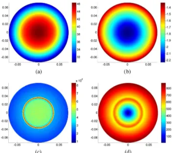
Fig. 4. Simulation results for the central axial slice of the first simulation phantom: (a) magnitude of , (b) phase of , (c) modulus of , (d) modulus of the convective field . Units for axes are meters. Modulus of the convective field has much lower value at the region around the center of the imaging slice, and this region is called as LCF region.

from to rather than from to ,

this term changes sign (assuming read-out direction is ). In this study, as suggested in [28], this fact is exploited for ob-taining as follows: Two phase images are acquired by using spin-echo pulse sequences of different read-out gradient polarities. Their phases are then summed and the resulting phase is halved to obtain . It is assumed that the transmit and receive phases of a quadrature birdcage coil are very close to each other, i.e., [25], and as a result of this approximation (transceive phase approximation), the phase of

is calculated as half of the transceive phase, i.e., .

Complete determination of requires the application of two gradient echo sequences and two spin echo sequences which altogether take min.

3) Obtaining on the Nodes of the Triangular Mesh: As

discussed above, the MREPT algorithm proposed in this study is triangular mesh based and it is required that is known on the nodes of the triangular mesh in the imaging slice. In order to obtain on the nodes of the triangular mesh, it is necessary that , , and the spin-echo MR images are reconstructed on the nodes as well. In a traditional MRI experiment, MR im-ages are obtained on a rectangular grid by the inverse FFT of the acquired k-space data. Instead, in this study, MR images are directly obtained on the nodes of the triangular mesh from the k-space data by evaluating the inverse discrete Fourier trans-form at the nodes: The value of a complex MR image at the th node, can be expressed as

(21) where denotes the raw data matrix, denotes the spa-tial frequency spacing in - and - directions ,

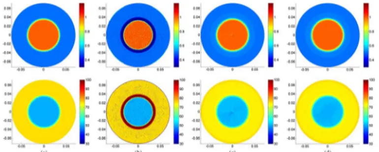
Fig. 5. Reconstruction results for the first simulation phantom: Upper row is for conductivity (S/m) and lower row is for relative permittivity : (a) true

, (b) reconstructed using the std-MREPT method, (c) reconstructed using cr-MREPT method, (d) reconstructed using the constrained cr-MREPT method. The spot-like artifact observed in (c) at the center is elim-inated when constrained cr-MREPT method is used as shown in (d). Units for axes are meters.

and denote the - and - coordinates of the th node, denotes the raw data matrix size, and denotes the number of nodes in the imaging slice.

IV. RESULTS

A. Simulation Results

1) The Constrained cr-MREPT and the Double-Excitation cr-MREPT Methods: In this section, we present results using

simulated data without additive noise. The cross-sectional view of the actual conductivity and permittivity distributions of the first simulation phantom which consist of two concentric cylin-ders are shown in Fig. 5(a). In the internal boundaries (transi-tion regions), the material properties change in a tapered fashion (not abruptly). The central slice of the phantom is chosen as the slice of interest, and the corresponding magni-tude, and phase distributions are shown in Fig. 4(a) and (b). distribution, and the modulus of the convective field, , are shown in Fig. 4(c) and (d) (note that since , ). It is observed that the distribution, as expected, has high magnitude in the tran-sition regions. It is also observed that the modulus of the con-vective field attains very low values around the center and in fact falls to zero at the center. Using these data, and distributions are reconstructed by applying both the std-MREPT method and also the cr-MREPT method that we have proposed.

The reconstructed and distributions obtained using the std-MREPT method are shown in Fig. 5(b) and Fig. 6(b) and (d). This method gives good reconstruction results in the regions where and do not vary but it yields severe errors in the transi-tion regions. This is because std-MREPT method assumes that spatial variations of and are small in the region of recon-struction and the term involving in (8) is not taken into account in this method.

Fig. 5(c) and Fig. 6(a) and (c) shows the results of the cr-MREPT method and the most important advantage of this method seems to be its ability to reliably reconstruct and distributions everywhere including the transition regions. On the other hand, cr-MREPT method seems to be ill-conditioned (not well-posed) at the origin where a spot-like artifact is observed. This artifact is mainly due to the numerical errors introduced by the region where the modulus of the convective

Fig. 6. Line profiles of the reconstructed and the actual conductivity along the x-axis for the first simulation phantom. (a) cr-MREPT and the constrained cr-MREPT are used for the reconstruction. (b) std-MREPT method is used for the reconstruction. (c) and (d) Reconstructed relative permittivity using the same methods as in (a) and (b). Spot-like artifact observed in cr-MREPT reconstruc-tions is eliminated when constrained cr-MREPT is used.

field [in (8)] is nearly zero [shown in Fig. 4(d)]. This region is referred to as the low convection field (LCF) region, and it corresponds to the region where z-component of the total current (conduction current displacement current) is small.

In order to eliminate the spot-like artifact, we propose two different methods. In the first method, called “constrained cr-MREPT,” we first determine the LCF region by observing the modulus of the convective field. In the LCF region, we re-construct and using the std-MREPT method [i.e., (9)] which is derived by ignoring the convection term in (8). Then, we apply the cr-MREPT method for the whole domain, whereby and found by the std-MREPT method in the LCF region are used as a priori knowledge (i.e., as constraint as explained in Section III-A. The resulting reconstructed and distributions, shown in Fig. 5(d), do not have spot-like artifacts in the LCF region which we have taken to be the circular region of radius 0.01 m at the center. This improvement in the reconstructions is also observed in the line profiles of reconstructed conduc-tivity and permitconduc-tivity shown in Fig. 6(a) and (c). However, this method does not give reliable reconstruction results when the LCF region coincides with the boundaries. This is simply because std-MREPT method gives unreliable estimates of the electrical properties in regions where they vary. To cover such cases we propose a second artifact-elimination method as explained below.

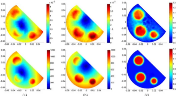
In the second method, called “double-excitation cr-MREPT,” and are reconstructed using together two different data that have different LCF regions. To explain and test this method the second simulation phantom shown in Fig. 3(b) is used. In this phantom there are three regions, C, D, and E. Regions D and E are the background regions and region C represents the anomaly region where and are different. This anomaly re-gion and its surrounding (union of rere-gions C and D) is our ROI. The actual and distributions in the ROI are shown in

Fig. 7. Moduli of the convective fields for the second simulation phantom using two different excitations: (a) region E is included (assigned the same material properties as region D), (b) region E is cut out (assigned material properties of air). ROI (regions C and D) is enclosed by a black border in (a). Convective fields shown in (a) and (b) have different LCF regions in the ROI. Units for axes are meters.

Fig. 8(a). We need to realize two different experiments in which the data in the ROI are different. This is achieved by in-cluding or exin-cluding region E in the simulations. In other words in one case region E is assigned the same material properties as for region D, and in the other case it is assumed to be cut out (or assigned material properties of air). Thus we obtain two dif-ferent data for the ROI by modifying the regions external to the ROI. The two different data, that also have different LCF in the ROI, are shown in Fig. 7(a) and (b). If these data are used separately for cr-MREPT method, the reconstructions shown in Fig. 9(a) and (b) are obtained and the spot-like arti-facts can be observed in the corresponding LCF regions. Using these data together, (8) is solved via (16) and the resulting reconstructed and distributions, shown in Fig. 9(c), do not have spot-like artifacts.

Fig. 8(b) shows the reconstruction results for the second exci-tation of the second simulation phantom using the std-MREPT method. As expected this method has unacceptable perfor-mance in the transition regions where the electrical properties are changing. On the other hand, Fig. 8(c) shows the same reconstructions for the second excitation when the constrained cr-MREPT method is used. Note that, as shown in Fig. 7(b), the LCF region for the second excitation is located inside the object where the electrical properties are constant. Therefore, in the LCF region, the std-MREPT method is used to obtain the electrical properties and the constrained cr-MREPT method is then applied in the whole solution domain including the transition regions resulting in successful reconstructions for both and . However, for the first excitation of the second simulation phantom, the LCF region coincides with an internal boundary where the electrical properties are changing as ob-served from Fig. 7(a) (This is also apparent from Fig. 9(a) where the spot-like artifact occurs at the transition region). In such cases, the std-MREPT method cannot be used in the LCF region and thus the constrained cr-MREPT method would fail to reconstruct the electrical properties in the whole solution domain.

2) Performance of the cr-MREPT Methods Against Noise:

The noise tolerance of the cr-MREPT method is investigated by using the second simulation phantom. For this purpose, noise is added to the simulated data as explained in Section III-B2 for SNR values of 150, 100, and 50. With noisy

Fig. 8. Reconstruction results for the second simulation phantom: Upper row is for conductivity (S/m) and lower row is for relative permittivity . (a) Actual electrical properties, (b) reconstructions using the std-MREPT method, (c) reconstructions using the constrained cr-MREPT method. Units for axes are meters.

Fig. 9. Reconstruction results for the second simulation phantom: Upper row is for conductivity (S/m) and lower row is for relative permittivity . cr-MREPT method is used (a) for only the first excitation and (b) for only the second excitation. (c) Double-excitation cr-MREPT method is used. The spot-like artifacts observed in (a) and (b) at different locations, are eliminated when double-excitation cr-MREPT method is used as shown in (c). Units for axes are meters.

data even for the reconstructed images become totally unacceptable to the extent that the anomaly region is not even distinguished. Therefore, the noise-added data is low pass filtered before reconstructions are made and the resulting reconstructions are shown in Fig. 10 and Fig. 11. For the noiseless but filtered data, the effect of filtering alone is observed in Fig. 11(a) where double-excitation cr-MREPT method is applied. As expected the transition regions are blunted and widened implying reduction of spatial resolution. (For this case, the relative errors for the reconstructed and are 6.2% and 3.3%, respectively, as shown in Table I. A significant portion of these errors are due to the low pass filter mentioned above. If the low-pass filter is not used, then for the noiseless case the corresponding relative errors are 2.3% and 1.9%. The filter tapers the variations of in the transition regions and consequently blunts the variations of and across the internal boundaries and thus relative errors increase). As shown in Fig. 10(a) and (b), despite the

use of filtering the single-excitation cr-MREPT reconstructions are grossly distorted even for . This distortion is mostly profound in and around the LCF regions. Constrained cr-MREPT method, on the other hand, gives acceptable recon-struction images [Fig. 10(c)] for when the second

Fig. 10. Reconstruction results of cr-MREPT when noise corresponding to SNR of 150 is added: cr-MREPT method is used (a) for only the first excita-tion and (b) for only the second excitaexcita-tion. (c) Constrained cr-MREPT method is used. Upper row is for conductivity (S/m) and lower row is for relative per-mittivity . Units for axes are meters.

Fig. 11. Double excitation cr-MREPT reconstruction results for the second simulation phantom when noise corresponding to SNRs of , 150, 100, or 50 is added to each data obtained for the two excitations. Upper row is for con-ductivity (S/m) and lower row is for relative permittivity . Units for axes are meters.

excitation data is used. Fig. 11 depicts the performance of the double-excitation cr-MREPT method for , 100, and 50. The relative errors in the reconstructed images using both the constrained and double-excitation cr-MREPT method for different SNR values are listed in Table I. In general, we have found that using the double-excitation cr-MREPT method, the artifacts appearing around the LCF region are significantly reduced except for very low SNR. Despite the use of double-excitation, as SNR is reduced, some systematic changes occur in and around the LCF regions. We think this is due to enlargement of the LCF regions as a result of interaction with noise. The constrained cr-MREPT is also successful but, as SNR is decreased, LCF region may spread into the transition regions making the application of constrained cr-MREPT unfeasible.

3) Effects of the Transceive Phase Approximation on cr-MREPT Reconstructions: The phase of the RF excitation

field , i.e., , is calculated exactly, within the limits of the numerical methods, and is used in MREPT algorithms when electrical property reconstructions are made from simulated data. However, in real experiments we cannot measure directly and we approximate it as half of the transceive phase,

. It is necessary to assess the effect of this TPA on the reconstructions. The cr-MREPT reconstructions obtained when the transmit phase is approximated as half of the transceive phase are shown in Fig. 12 for the second simulation phantom.

TABLE I

ERRORS IN AND RECONSTRUCTEDUSING THE CR-MREPT METHODS

WHENNOISECORRESPONDING TODIFFERENTSNR VALUES AREADDED TO (LPF: LOWPASSFILTER)

Fig. 12. Effect of TPA on cr-MREPT reconstructions. (a) Noise-free case with double-excitation cr-MREPT method, (b) case with double excita-tion cr-MREPT method, and (c) case with constrained cr-MREPT method. Units for axes are meters.

For the noiseless case, using the double-excitation cr-MREPT method, reconstructions are shown in Fig. 12(a). It is found that and values in the inner object vary between 0.92–1.08 S/m and 46–63, respectively. If TPA is not applied, as mea-sured from the reconstructions shown in Fig. 9(c), the and values in the inner object vary between 0.98–1.02 S/m and 54–48, respectively. The increased variation observed with the introduction of TPA is in the form of a low frequency trend. However the success of cr-MREPT in reconstructing transition regions is not lost when TPA is used. For the

case, reconstructions of both the double-excitation and the con-strained cr-MREPT methods, as shown in Fig. 12(b) and (c), are effected by TPA again by the introduction of low frequency trends. The relative errors in the reconstructions with the TPA are given in Table II, and when compared with the results of Table I (which has the results without TPA) it is observed that the relative errors somewhat increase, but are still in the same range especially when noisy data is used.

4) Application of the cr-MREPT Method to a Head Model:

In order to observe the performance of the cr-MREPT method under more realistic conditions we have applied it to a head model. Fig. 13 has a 2-D axial brain slice segmented into five tissues, namely, cerebro spinal fluid (CSF), white matter (WM), gray matter (GM), skull, and scalp. Table III has the electrical properties assigned to these tissues. Also in Fig. 13 a padding re-gion is shown which is assumed to be padded to the head in order to obtain measurements of a second excitation. This padding is assigned a conductivity value close to that of gray matter, and a

TABLE II

ERRORS IN AND RECONSTRUCTED BY THE CR-MREPT METHODS

WHENNOISECORRESPONDING TODIFFERENTSNR VALUES AREADDED TO ANDWHENTPAISUSED. (LPF: LOWPASSFILTER)

Fig. 13. Illustration of the simplified head model and the pad which is attached to one side of the head.

TABLE III

ELECTRICALPROPERTIES OF THEHEADMODEL AND THEPAD

permittivity value of slightly higher than CSF. Simulations are performed using the same birdcage coil given in Fig. 2. The 2-D head slice with padding shown in Fig. 13 is extruded in z-direc-tion, by 17.5 cm, to form a 3-D geometry and the final 3-D ob-ject is placed in the birdcage coil. Fig. 14(b)–(e) depicts the re-sults of cr-MREPT for the first excitation (i.e., without padding), cr-MREPT for the second excitation (i.e., with padding), double excitation cr-MREPT, and constrained cr-MREPT for the first excitation, respectively. As seen in Fig. 14(b) and (c) the pres-ence of padding significantly shifts the LCF region as apparent from the shift of the spot-like artifact observed for single excita-tion cr-MREPT reconstrucexcita-tions. Both the double-excitaexcita-tion and constrained cr-MREPT methods give very satisfactory results especially for the conductivity. The permittivity reconstructions have more error especially in the CSF regions which have higher

and .

In the reconstruction results given in Fig. 14, the transmit phase is assumed to be known. The effect of TPA on the cr-MREPT reconstructions is also investigated for the head

model. Fig. 15(a) and (b) shows the actual transmit phase and the error introduced by TPA for the excitations without and with padding, respectively. Without padding the error in the transmit phase introduced by TPA is about and it increases to increased when padding is used. Fig. 15(c) and (d) shows the reconstructions obtained when TPA is applied when using double-excitation cr-MREPT, and constrained cr-MREPT for the first excitation, respectively. The relative errors in the reconstructions with and without the transceive phase approximation are given in Table IV. With the TPA, the relative error is slightly increased for the conductivity and there is no observable difference comparing the reconstructed conductivities in Fig. 14(d) and (e) with the ones in Fig. 15(c) and (d). However, the impact of TPA on the permittivity reconstructions seems to be higher as evident from the relative error values in Table IV. Especially in the CSF region, where the and are higher, the error is introduced in permittivity by TPA is more apparent as shown in Fig. 15(c) and (d). Fig. 15(e) shows the reconstruction results when noise is added to the simulated data of the head model in an amount corresponding to an MR SNR of 100, and TPA is also applied. As before, when noise is added, a low pass filter with Gaussian kernel with standard deviation 0.0032 m is applied before reconstructions are undertaken. It is observed that the noise is very well tolerated by the cr-MREPT algorithm and however due to filtering transition regions are widened.

B. Experimental Results

Experiments are first conducted using the first experimental phantom. The same low pass filter, which is used for noisy sim-ulated data as mentioned above, is applied also to the measured

. Fig. 16(a) and (b) shows the measured and filtered magnitude and phase . Fig. 16(c) and (d) shows the modulus of , and the modulus of the convective field ob-tained from the filtered . In obtaining we have also eliminated the phase accumulated due to the eddy-cur-rents as explained in Section III-C2. For comparison purposes, half of the phase accumulated due to the eddy currents, i.e., , and half of the phase of the spin-echo image, , are shown in Fig. 16(e) and (f), respectively. It is observed that the phase accumulated due to the eddy currents is significant (peak to peak level of 0.4 rad) compared to (peak-to-peak level of 0.7 rad). These results justify the need for the elimination of eddy current induced phase when finding

.

Reconstructed conductivity distributions are first obtained by applying std-MREPT and Voigt’s methods which are explained in the introduction, and are shown in Fig. 17(a) and (b), respec-tively. Similar to the simulation case, the result of std-MREPT method has severe errors on the internal boundaries. Since std-MREPT method is a point-wise method and it depends on the second derivatives of , this method is very sensitive to noise and the reconstructed conductivity distribution is very noisy, as shown in Fig. 17(a). However, since Voigt’s method has an in-tegral based formula and it depends on the first derivatives of only, this method gives a less noisy reconstruction result as shown in Fig. 17(b). Voigt’s method still has severe errors in the transition regions.

Fig. 14. Reconstruction results for the head model (Upper row is for conductivity (S/m) and lower row is for relative permittivity ). (a) Actual electrical properties. (b) cr-MREPT reconstructions using the first excitation. (c) cr-MREPT reconstructions using the second excitation. (d) Double-excitation cr-MREPT method results. (e) Constrained cr-MREPT method results. Units for axes are meters.

Fig. 15. Effect of TPA on cr-MREPT reconstructions of the head model. (a) Actual transmit phase (upper plot) and error due to phase approximation (lower plot) without padding (both in degrees). (b) Actual transmit phase (upper plot) and error due to phase approximation (lower plot) with padding (both in degrees). Reconstructed conductivity (S/m) and relative permittivity when (c) double-excitation cr-MREPT, and (d) constrained cr-MREPT is used. (e) Results of double-excitation cr-MREPT applied to noisy simulated data after low pass filtering. Units for axes are meters.

TABLE IV

EFFECT OFTPAFOR THEBRAINMODEL ERRORS IN AND

On the other hand, cr-MREPT is very successful in recon-structing the boundary transitions as shown in Fig. 17(c). How-ever, the result of cr-MREPT method has a spot-like artifact in the LCF region. When the constrained cr-MREPT method, which is explained in Section IV-A, is applied, the reconstructed conductivity shown in Fig. 17(d) is obtained and it does not have

a spot-like artifact. In this method, a circular region with radius of 0.007 m which encloses the spot-like artifact region is first selected. In this region, the averages of the electrical proper-ties found using std-MREPT method are calculated. These av-erage values are used for this region as a constraint (a priori knowledge) in the constrained cr-MREPT method. The average conductivity values for the reconstructed distribution shown in Fig. 17(d) are 0.93 S/m for the inner object and 0.43 S/m for the background. These values are consistent with the estimated values given in the section on phantom preparation. When ap-plying the cr-MREPT method, the average conductivity and per-mittivity values obtained by the std-MREPT method at the outer boundary are used for assigning the Dirichlet boundary condi-tion required in solving (8).

Experiments are then performed using the second experi-mental phantom. Fig. 18(a) and (b) shows the moduli of the

Fig. 16. For the axial slice of the first experimental phantom, (a) magnitude of (Tesla), (b) phase of (rads), (c) modulus of , (d) modulus of the convective field (T/m), (e) half of the phase accumulated due to the eddy currents, (f) half of the transmit phase if the eddy-current phase is not eliminated. Units for axes are meters.

Fig. 17. Reconstructed conductivity distributions for the first experimental phantom using (a) std-MREPT method, (b) Voigt’s method, (c) cr-MREPT method, (d) constrained cr-MREPT method. Units for axes are meters.

convective fields for the first and second excitations which are obtained with and without segment E, respectively. As shown in Fig. 18, these convective fields have different LCF regions that do not coincide with each other. Using the calculated data of the two cases together, double excitation cr-MREPT method is applied and the reconstructed conductivity distri-bution is obtained, as shown in Fig. 18(c). Outer boundary conditions are again taken from the results of the std-MREPT method. As expected, the reconstructed conductivity distri-bution does not have spot-like artifacts, and the boundary transitions are well constructed. The average reconstructed conductivity values are 0.99 S/m for the inner object and 0.45 S/m for the background, again similar to the estimated values.

We have also conducted experiments with the third experi-mental phantom which has relatively more complex geometry, as shown in Fig. 3(c). For the conductivity reconstruction, the

double-excitation cr-MREPT method is applied. For compar-ison, the same phantom geometry is also modeled in the sim-ulation environment and the conductivity is reconstructed. Top row of Fig. 19(a) and (b) shows the modulus of the convec-tive field calculated using the experimental data for the first and second excitation, respectively, whereas in the bottom row the convective fields calculated in the simulations are shown. A low pass filter with Gaussian kernel with standard deviation 0.0032 m is applied when processing both the simulated and the ex-perimental data. It is observed that the convective field distri-butions in the experiments and in the simulations have similar trends, and in the second excitation the location of the LCF gion is similarly shifted. Fig. 19(c) shows the conductivity re-constructions obtained using the experimental data (top row) and using the simulated data (bottom row). The average recon-structed conductivity values are 1.22 S/m for the inner objects and 0.62 S/m for the background, again similar to the estimated values.

V. DISCUSSION

Previously developed practical MREPT algorithms recon-struct electrical properties in regions where and values vary slowly [25], [26], [28]. In this study, we have proposed a novel algorithm named convection-reaction equation based MREPT (cr-MREPT) which reconstructs and also in transition re-gions such as boundaries of internal objects. However, spot-like artifacts are observed in the LCF regions where the convection field is low. To eliminate these artifacts, we have proposed two different methods named as “constrained cr-MREPT” and “double-excitation cr-MREPT.” We have validated these MREPT methods using both simulated and experimental data.

The “constrained cr-MREPT” method has the advantage that it can be applied even for single-excitation data but it has the limitation that it cannot be applied in the LCF re-gions which have varying and . The “double-excitation cr-MREPT” method, however, can be applied to such cases as well. In double-excitation cr-MREPT two different measurements are obtained such that the LCF regions are different. In this study, we have proposed “padding” to obtain two different excitations, one obtained without padding and the other obtained with padding. In our experimental studies, we have realized “padding” by cutting part of the phantoms and then repeating the experiments. In our head simulation phantom, we have envisaged that padding material is attached to one side of the head. We have obtained successful recon-structions with the head phantom using padding material, the electrical properties of which are not very different from the electrical properties of head tissues. Studies which have used passive materials to improve aspects of MRI by effecting the distribution of radio-frequency electromagnetic fields, have led to the development of padding materials in the form of gels and slurries [55]–[57]. Although many of such padding materials are of low conductivity and high permittivity, high conductivity gels (17 g/L NaCl) have also been proposed and used [57]. Conductive padding, in general, compromises SNR [57]. However for the purpose of altering the position of the LCF region, our preliminary studies indicate that conductive padding may be more instrumental. Another effect of padding

Fig. 18. For the central axial slice of the second experimental phantom, (a) modulus of the convective field (T/m) for the first excitation, (b) modulus of the convective field (T/m) for the second excitation, (c) reconstructed conduc-tivity (S/m) distribution using double-excitation cr-MREPT method. Convec-tive fields shown in (a) and (b) have different LCF regions. Units for axes are meters.

Fig. 19. For the central axial slice of the third phantom, experimental (upper row) and simulated (lower row) (a) modulus of convective field for the first excitation, (b) modulus of convective field for the second excitation, (c) re-constructed conductivity (S/m) distributions when double-excitation cr-MREPT method is used. Units for axes are meters. Top row convective field units are T/m and bottom row convective field units are .

which must be taken into consideration is whether the TPA is still applicable when padding is used. The results that we have presented in Section IV-A4 show that, at least for the head phantom and the padding material that we have used in this section, the TPA is still applicable. Although the determination of the exact shape, position, material, and electrical properties of a contacting object to be used for padding is the subject of further studies, the results we have demonstrated in this paper show that double-excitation cr-MREPT using padding is a feasible technique.

In order to realize a second excitation for the double-ex-citation cr-MREPT method, instead of padding an additional transmit channel (coil) may be used so that the LCF region is shifted. To set up a second matrix equation, as in (15) and (16), we need to obtain the complex map for the additional coil. If this coil is used for both transmit and receive, then the transceive phase approximation may not hold. As a matter of fact, to the knowledge of the authors, a birdcage coil driven in quadrature mode (or some of its variants like the TEM coil), is the only coil configuration for which the TPA is applicable. As a solution to this problem, for the second excitation one may transmit from the additional coil and receive from the birdcage coil, since the receive phase of the birdcage coil is already known from the first excitation data. It must be noted however that in designing the additional coil one must also be careful about minimizing in the slice of interest. The design and application of additional coils for double excitation cr-MREPT will be the focus of future studies.

In this study, the derived convection-reaction equation of MREPT is solved using a triangular mesh based finite differ-ence method. We have used the mesh generation facility of COMSOL Multiphysics in order to obtain a triangular mesh. The solution of the equation itself can also be done by FEM or other numerical methods. In our previous studies, we developed a convection equation-based formulation for MREIT and its numerical solution was based on FEM [58]. Some specific problems which arise when a commercial FEM package is used for the solution are discussed in [58]. We have also applied a FEM-based solution method for constrained cr-MREPT [59]. The extension of FEM to the double excitation cr-MREPT and the use of regularization and stabilization methods will be considered in future studies.

Mesh size is an important factor from the point of view of artifacts and errors. We have found that the spot-like artifact which appears in LCF regions, when especially single-excita-tion cr-MREPT is used, can be significantly eliminated in the simulations if a very fine mesh is used. One reason for this is that using a fine mesh the solution of the fields become more accurate but another reason is that the first and second deriva-tives of are also calculated more accurately. We have ob-served this behavior especially when we used some 2-D sim-ulations where we can make the mesh extremely fine (element size of 0.2 mm). In such cases the spot like artifact disappears almost completely even in single-excitation cr-MREPT. Also, when high resolution 2-D simulations were made using the head phantom the errors that we have observed especially for the per-mittivity reconstructions shown in Figs. 14 and 15 disappeared. However, using an extremely fine mesh may not be feasible nor useful in practice because of several reasons. 1) When simula-tions involving the solution of the forward problem for the 3-D loaded birdcage coil are considered, excessive memory require-ments arise as explained below. 2) Although an extremely fine mesh eliminates the spot-like artifacts for the noise-free cases, these artifacts reappear when noise is added to the data. 3) For experimental data the resolution is determined by the resolution of the MR system and therefore in the calculation of the first and second derivatives of we are limited by the MR res-olution anyway. In our forward problem simulations, we have used a mesh element size of 1 mm in the slices of interest for the first, second, and third simulation phantoms whereas for the head model 1.4 mm is used. Mesh element size is increased gradually for more distant slices in order to meet the memory requirements. For example, for the first three simulation phan-toms the number of degrees-of-freedom was 11,048,442 and 55 GB RAM was necessary. We have used HP Z800 workstation with Intel Zeon X5675 3.07 GHz dual processors (12 cores) and with 64 GB RAM. Thus it was not possible to use finer meshes. Solution of one forward problem took 43 min. In solving the in-verse problem, we did not have any memory problem since re-constructions were made only for the slice of interest and 41619 elements were sufficient. One complete admittivity reconstruc-tion, including the low-pass filtering of , calculation of the derivatives of , and solving (16) took 225 s.

Noise tolerance of our algorithm is also investigated for different noise levels. Since the Laplacian operation, used in finding , amplifies the noise, the cr-MREPT method is

relatively sensitive to noise. A low pass filter with Gaussian kernel with standard deviation 0.0032 m is applied when processing both the noisy simulated data and the experimental data. This filtering causes the transition regions, where elec-trical properties vary, to appear wider in the reconstructed images. Therefore, in determining the standard deviation of the Gaussian kernel, this tradeoff between having less noisy reconstructions and having higher spatial resolution must be taken into consideration.

In this study, we used the TPA to estimate the phase of the field, since we used a quadrature birdcage coil. In fact, the limits of the TPA have been studied for the birdcage coil and it has been argued that the phase is exactly equal to half the transceive phase in some situations, e.g., circular sym-metry in electrical properties [25], [26], [28], [29]. Recently, several groups have investigated the mapping of the transmit phase for multi-channel transmit/receive coil arrays. In these studies, the transmit or receive phase distribution of a certain coil is taken as reference and all the other phases are deter-mined with respect to this [30], [31], [34]. These studies also involve the reconstruction of electrical properties, but their al-gorithms are confined to regions where the electrical properties vary slowly. Another recent study using a multi-channel array, has addressed the problem of reconstruction also in transition regions, but it must still be assessed under real experimental conditions [35]. The cr-MREPT method that we have devel-oped successfully handles the reconstruction in the transition regions and it is applicable to the widely-used birdcage coil. Furthermore, since multiple distributions can be obtained using a multi-channel array, and since their LCF regions may be different, the cr-MREPT method can be applied, to advan-tage, using all these distributions simultaneously. Further research is needed on this topic.

In the cr-MREPT algorithm, the z-component of the magnetic field intensity is neglected. In the case of a RF birdcage coil, is generated mainly by the end-rings of the RF birdcage coil. In the central slice, the magnitude of is small in the following two cases. 1) generated by the end-rings of the opposite sides mostly cancel each other at the central slice especially for a symmetric situation in the z-direction with respect to the central slice. 2) The end-rings are far away from the central slice. In our simulation and experimental phantoms, there is z-symmetry and also the end-rings are distant from the central slice since we have used a body coil. Errors in MREPT measurements gradually increase as slices move off-center, especially if short birdcage coils are used. This limits the applicability of the technique for multi-slice MREPT especially using short head coils which are preferable for SNR purposes. It has been argued by Zhang et al. that when TEM coils, which do not have end-ring currents, are used, better reconstruction results with higher accuracy can be obtained [27]. Another suggestion for minimizing effects is made by Katscher et al., who propose to estimate from a full model including the birdcage coil and the patient, and/or to find it by iterative computation [32].

In our simulation and experimental studies, we have used phantoms which are geometrically (electrically) invariant in the z-direction. Variations in z-direction, such as in in vivo appli-cations might be expected to influence the accuracy of results.

In this study we have not addressed this issue. If z-variation does not occur exactly on the imaging slice then as can be seen from (7), drops and the slice imaging problem reduces to 2-D. In other words, z-variations distant from the slice of in-terest do not affect the cr-MREPT reconstructions for that slice. If z-variation is exactly on the slice of interest, then several ap-proaches might be suggested.1) Equation (7) can be handled as a 3-D problem provided that multi-slice data is acquired and the boundary conditions for the 3-D ROI are properly assigned. 2) Data from two excitations can be used such that two different sets of coefficients for (7) are obtained. By an appropriate linear combination of the two equations, the variable can be eliminated.

In experimental studies, we have used the double angle method for mapping. In order to reduce the acquisition times, other mapping techniques such as actual flip angle imaging (AFI) [53], Multiple mapping (MTM) [52], and Bloch–Siegert shift based mapping [54] can be used. For example, Voigt et al. have used MTM and have achieved a total acquisition time of 16 min with eight averages in in vivo experiments [29]. Bulumulla et al. have used Bloch–Siegert shift based mapping [60]. We know from Sacolick et al., who have developed the Bloch–Siegert shift based mapping technique, that a single mapping can be completed in 18 s [54]. For the measurement of the phase of distributions we have used a SE sequence. However, Stehning et al. have used SSFP for phase measurement and this sequence takes less than a minute even for multi-slice and with multiple averaging [61]. In conclusion, significant reduction in total acquisition for complex map is possible and is essential for in vivo applications.

VI. CONCLUSION

This study substantially improves the MREPT technique by proposing a novel method, cr-MREPT, which is capable of re-constructing conductivity and dielectric permittivity not only in regions where they vary slowly but also where they have high gradients. It has been shown that the proposed method is appli-cable in a standard MRI system using a quadrature birdcage coil. The method performs well against noise, against the transceive phase approximation and for complex electrical property distri-butions such as in the head. Further studies are needed to inves-tigate the suitability of the cr-MREPT to real-life applications specifically in relation to padding structures and multi-coil con-figurations.

REFERENCES

[1] C. Gabriel, S. Gabriel, and E. Courhout, “The dielectric properties of biological tissues: I. Literature survey,” Phys. Med. Biol., vol. 41, pp. 2231–2249, Nov. 1996.

[2] E. C. Fear, X. Li, S. C. Hagness, and M. A. Stuchly, “Confocal mi-crowave imaging for the breast cancer detection: Localization of tu-mors in three dimensions,” IEEE Trans. Biomed. Eng., vol. 49, no. 8, pp. 812–822, Aug. 2002.

[3] W. T. Joines, Y. Zhang, C. Li, and R. L. Jirtle, “The measured elec-trical properties of normal and malignant human tissues from 50 to 900 MHz,” Med. Phys., vol. 21, pp. 547–550, Apr. 1994.

[4] A. J. Surowiec, S. S. Stuchly, J. B. Barr, and A. Swarup, “Dielec-tric properties of breast carcinoma and the surrounding tissues,” IEEE