Selçuk J. Appl. Math. Selçuk Journal of Vol. 8. No.2. pp. 3 - 12 , 2007 Applied Mathematics
A New Epsilon-Local Dependence Measure and Dependence Maps
Burcu H. Ucer1and Ismihan Bayramoglu2
1Dokuz Eylul University, Faculty of Arts and Sciences, Department of Statistics,
35160, Buca, Izmir, Turkey; e-mail:burcu.hudaverdi@ deu.edu.tr
2Izmir University of Economics, Faculty of Sciences and Literature, Department of
Mathematics, 35330, Balcova, Izmir, Turkey; e-mail:ism ihan.bayram oglu@ ieu.edu.tr
Received : March 28, 2007
Summary. In the present work, we introduce a new local dependence func-tion characterizing dependence structure between two random variables in an −neighborhood of a particular point from the domain of underlying bivariate distribution and investigate its properties. As an example the local depen-dence function for Farlie-Gumbel-Morgenstern distribution is provided. Also, we construct dependence maps for some pairs of random variables. We use the estimator of local dependence function to construct the dependence map. Per-mutation test algorithm is applied for = 500 to obtain more accurate result in dependence map and also several examples are provided.
Key words:Local dependence function, permutation test, dependence map 1. Introduction
The concept of dependence among random variables is necessary in statisti-cal theory and applications. Unless specific assumptions are made about the dependence no meaningful statistical model can be constructed. The Pearson correlation coefficient and many other scalar dependence measures, of course, play an important role in understanding the simplest dependence relationships between two random variables. In general, the dependence structure between a pair of random variables is very complex and the scalar dependence measures can not be adequate to explain the natural association between them.
The study of the local dependence between random variables has attracted some interest in last years. There are several local dependence measures introduced and studied in statistical literature in the past decade. Bjerve and Doksum (1993) and Blyth (1994b) constructed a "correlation curve" that measures the
strength of the association between random variables locally. Holland and Wang (1987) introduced the local dependence function, which is a localized version of the Pearson correlation coefficient and is the second order partial derivative of logarithm of the bivariate density function. Jones (1996) has provided an alternative motivation for studying this function. Bairamov and Kotz (2000) have introduced a new local dependence function based on regression concept which is a radical generalization of the Pearson correlation coefficient. Because of the difficulty in interpreting the estimated local dependence function, Jones and Koch (2003) use the dependence maps via local permutation testing by using Holland and Wang’s (1987) local dependence function.
We introduce a new local dependence function that characterizes the dependence between two random variables in the −neighborhood of a particular point. This local dependence function is essentially different from all local dependence functions introduced earlier, because it depends on the point itself as well as the − which depends on the nature of the considered model. The local dependence function in the present paper is constructed by the natural way considering the localized version of the Hoeffding’s formula and possesses all properties that must satisfy any dependence measure.
Using the local dependence functions one can construct the dependence maps that make it possible to interpret the full dependence structure of the data set. Dependence maps help us to determine the dependence structure between ran-dom variables visually. Local dependence function becomes more interpretable tool through dependence maps. A dependence map is generally separated into three regions: positive (significant), negative (significant) and zero (nonsignifi-cant) regions. So, by the help of dependence maps we can easily interpret the dependence structure of the data. We construct the dependence map of the given data set by using the natural estimators of local dependence functions. Permutation test algorithm is developed by Visual Basic Script and applied for approximately 500 times to obtain accurate results. Several examples, con-cerning inflation with percentage change in ISE-100 Index and with percentage change in US Dollar and also simulated bivariate normal data are provided. 2.−Local Dependence Function
Let and be continuous random variables with distribution function ( ) and marginals () and (), respectively with support The function 12( ) is a local dependence function of and at the (1 2) neigh-borhood of the point ( ) ∈ The localized version of Hoeffding’s formula can be written as 12( ) = +Z 2 −2 +Z 1 −1 [( ) − ()()] p ()p ( )
We call this function as the −local dependence function. If the support of and is finite interval [ ] then it is clear that
12( ) = min(+Z 2) max(−2) min(+Z 1) max(−1) [( ) − ()()] p ()p ( )
2.1.Properties of the− Local Dependence Function
1.If and are independent, then 12( ) = 0 for all ( ) Proof: If and are independent then the bivariate distribution function is ( ) = ()()So, 12( ) = +Z 2 −2 +Z 1 −1 [()() − ()()] = 0 then 12( ) = 0 2.¯¯12( )¯¯ ≤ 1 for all ( ) Proof: It is known that
| ( )| = ¯ ¯ ¯ ¯ ¯ ¯ ¯ ¯ ¯ ¯ ¯ ¯ Z Z [( ) − ()()] q ()p ( ) ¯ ¯ ¯ ¯ ¯ ¯ ¯ ¯ ¯ ¯ ¯ ¯ ≤ 1
If the support of and is finite interval [ ] then the local depen-dence, ¯ ¯12( )¯¯ = ¯ ¯ ¯ ¯ ¯ ¯ ¯ ¯ ¯ ¯ ¯ ¯ ¯ +Z 1 −1 +Z 1 −1 [( ) − ()()] q ()p ( ) ¯ ¯ ¯ ¯ ¯ ¯ ¯ ¯ ¯ ¯ ¯ ¯ ¯ ≤ 1
3.If e = + and e = +, then 12(˜ ˜) = 12 ( )So
12(˜ ˜) = 12( ) where ˜ = + and ˜ = + Proof: ( ) = n ≤ ee ≤ o= { + ≤ + ≤ } = ½ ≤ − ≤ − ¾ = µ − − ¶ () = n ≤ e o= { + ≤ } = ½ ≤ − ¾ = µ − ¶ () = n ≤ e o= { + ≤ } = ½ ≤ − ¾ = µ − ¶ 1 2(˜ ˜) = ˜ +Z 2 ˜ −2 ˜ +Z 1 ˜ −1 [ ( ) − ()()] = ˜ +Z 2 ˜ −2 ˜ +Z 1 ˜ −1 [( − − ) − ( − )( − )] By using transformation, − = and − =
1 2(˜ ˜) = ˜ +2− Z ˜ −2− ˜ +1− Z ˜ −1− [( ) − ()()] = +Z2 −2 +Z1 −1 [( ) − ()()] = 2 ( ) so, 1 2 (˜ ˜) = 2 ( ) p ()p ( ) = 2 ( )
2.1.1.Example: Farlie-Gumbel-Morgenstern Copula
Consider Farlie-Gumbel-Morgenstern distributions with uniform marginals. The p.d.f. (Bairamov and Kotz, 2002) is
( ) = 1 + (1 −2)(1 −2) 0 ≤ ≤ 1 0 ≤ ≤ 1 −1 ≤ ≤ 1 Let 1= 2= then the local covariance function is
( ) = min(1+)Z max(0−) min(1+)Z max(0−) (1 − )(1 − ) = ∙µ 22 2 − 32 3 ¶ − µ 21 2 − 31 3 ¶¸ ∙µ 22 2 − 23 3 ¶ − µ 12 2 − 13 3 ¶¸ where 2 = min(1 + ) = ½ 1 1 − + 1 − 2 = min(1 + ) = ½ 1 1 − + 1 − 1 = max(0 − ) = ½ − 0 1 = max(0 − ) = ½ − 0
For simplicity denote = ( ) = ⎧ ⎪ ⎪ ⎪ ⎪ ⎪ ⎪ ⎪ ⎪ ⎪ ⎪ ⎪ ⎪ ⎪ ⎪ ⎪ ⎪ ⎪ ⎪ ⎪ ⎪ ⎪ ⎪ ⎪ ⎪ ⎪ ⎪ ⎪ ⎪ ⎪ ⎪ ⎪ ⎪ ⎪ ⎪ ⎪ ⎪ ⎪ ⎪ ⎪ ⎪ ⎪ ⎪ ⎨ ⎪ ⎪ ⎪ ⎪ ⎪ ⎪ ⎪ ⎪ ⎪ ⎪ ⎪ ⎪ ⎪ ⎪ ⎪ ⎪ ⎪ ⎪ ⎪ ⎪ ⎪ ⎪ ⎪ ⎪ ⎪ ⎪ ⎪ ⎪ ⎪ ⎪ ⎪ ⎪ ⎪ ⎪ ⎪ ⎪ ⎪ ⎪ ⎪ ⎪ ⎪ ⎪ ⎩ h(+)2 2 −(+)3 3i h(+)2 2 −(+)3 3i 0 0 h³(+)2 2 −(+)3 3´−³(−)2 2 −(−)3 3´i h(+)2 2 −(+)3 3i 1 − 0 h16−³(−)2 2 −(−)3 3´i h(+)2 2 −(+)3 3i 1 − 1 0 h(+)2 2 −(+)3 3i h³(+)2 2 −(+)3 3´−³(−)2 2 −(−)3 3´i 0 1 − h³(+)2 2 −(+)3 3´−³(−)2 2 −(−)3 3´i ⎡ ⎣ ³ (+)2 2 − (+)3 3 ´ −³(−)2 2 − (−)3 3 ´ ⎤ ⎦ 1 − 1 − h16−³(−)2 2 −(−)3 3´i h³(+)2 2 −(+)3 3´−³(−)2 2 −(−)3 3´i 1 − 1 1 − h(+)2 2 −(+)3 3i h1 6− ³( −)2 2 − (−)3 3 ´i 0 1 − 1 h³(+)2 2 −(+)3 3´−³(−)2 2 −(−)3 3´i h1 6− ³( −)2 2 − (−)3 3 ´i 1 − 1 − 1 h16 −³(−)2 2 −(−)3 3´i h16−³(−)2 2−(−)3 3´i 1 − 1 1 − 1
In Figure 1, we have presented graphs of local dependence function for FGM dis-tributions with different values of . It can be observed that lim
→1( ) =
3, which is the correlation coefficient of FGM distribution.
Figure 1 Graphs for Local dependence function of FGM Distribution for the different values of , = 05, = = 121
2.2.Estimation of ( )
We estimate the local dependence function for the data available such as
∗12( ) = 1 X =1
[max(+)−max(−)][max(+)−max(−)]
− 1 X =1 [max(+)−max(−)] 1 X =1 [max(+)−max(−)] Proof: ∗12( ) = +R 2 −2 +R 1 −1 [∗ ( ) − ∗()∗()] = +R 2 −2 +R 1 −1 ∙ 1 P =1 {≤ ≤}−¡1 P =1{≤} ¢ ¡1 P =1{ ≤} ¢¸ =1 P =1 max(R+2) max(−2) max(R+1) max(−1) − à 1 P =1 max(R+1) max(−1) ! à 1 P =1 max(R+2) max(−2) ! =1 P =1
[max ( + ) − max ( − )] [max ( + ) − max ( − )] −1 P =1 [max ( + ) − max ( − )] ×1 P =1 [max ( + ) − max ( − )] where ∗ ( ) = 1 X =1 {≤≤} ∗() = 1 X =1 {≤} and ∗() = 1 X =1 {≤}
where is an indicator function i.e.
() = ½
1 ∈ 0 ∈
and is the observation number and and are the sample standard deviations of and nespectively. By using this formula, we can compute the sample local dependence function as
∗12( ) = ∗
12( )
2.3.Local Permutation Test
Permutation test interests the variables being correlated can be classified on certain attributes, primarily. This test is a type of statistical significance test and based on permuting the observed data points across all possible outcomes. In local permutation testing, for each ( ), we firstly compute ˆ( ) for an appropriate −value firstly. We consider making local permutation test by comparing these original estimated values. We randomly permute to obtain new samples satisfying the independence hypothesis, which is ˆ( ) = 0 This permutation operation is repeated times, so we obtain samples which are satisfying the null hypothesis. ˆ is computed for each permuted data set, = 1 . For each permuted data set, the significant estimated local corre-lations at the −neighborhood are taken to the list by comparing the original estimated local correlations. The simulated local correlations in this list are ranked. At significance level, we decide the dependence map value, such that if the observed value of ˆ is in the highest (2)% of simulated ˆ ’s then the dependence map value is +1, if the observed value of ˆ is in the lowest (2)% of simulated ˆ ’s then the dependence map value is -1, otherwise it equals to 0. We take = 500, since the construction of dependence map does not change for the value greater than = 500. Also we prefer = 005 level to test the significance. We develop an application with Excel Visual Basic which is the application of the local permutation test.
2.3.1.Examples:
Standard Bivariate Normal Data We generate a standard-normal distrib-uted data set for = 100 and plot the dependence map for different values of For this data set, the Pearson correlation coefficient which measures the linear global correlation coefficient is 0.87. In Figure 2, there is wide positive region in spite of a small = 001 since dependence between and is strong; but also zero region is exist. For moderate values of and , it can be said that there is positive dependence. We can easily say that as increases, it approximates to the Pearson correlation coefficient. For = 1 we generally see positive de-pendence between and as expected; but also for large values of and and small values of and we see that there is independence.
Figure 2 Dependence map for Standard Bivariate Normal Data; zero local dependence is light grey, positive local dependence is white for = 001 1
Percentage Change in CPI - Percentage Change in US Dollar In this example, we concern that the dependence between monthly percentage change in consumer price index and monthly percentage change in US dollar between the years 1995-2005 for Turkey. There is not strong linear correlation for = 0314. In Figure 3, we see that for = 25, dollar percentage changes around zero is positively dependent with inflation. Also we see that when = 95, there is generally positive dependence except from the lowest and highest values of percentage change in dollar, because there is independence at the lowest and the highest values of change in dollar.
Figure 3 Dependence map for Consumer Price Index monthly change rate and dollar monthly change rate; zero local dependence is light grey, positive
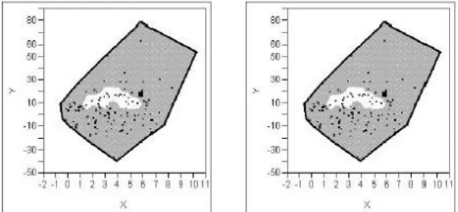
local dependence is white for = 25 95( : inflation, : dollar) Percentage Change in CPI -Percentage Change in ISE-100In this ex-ample,we investigate the dependence structure between the variables, monthly percentage change in consumer price index and monthly percentage change in Istanbul Stock Exchange-100 index. In Figure 3, in the case that = 25, there is small positive region that is for the percentage changes in ISE-100 around 10, but there is generally independence. When gets larger, it does not effect the dependence structure very much since there is weak dependence between and
Figure 4 Dependence map for consumer price index monthly change rate and ISE-100 monthly change rate; zero local dependence is light grey; positive local dependence is white for = 25 15. ( : inflation, : ISE-100) 3.Conclusions
In a way that global statistic measure cannot be enough to explain the real dependence structure of the data; instead local measures of dependence can be used. Dependence maps provide to interpret easily the dependence structure of the data. We provide an algorithm of the local permutation test to construct dependence maps. We use −local dependence measure that reveals the natural dependence between the variables by clustering ( ) according to the cho-sen We also provide several examples that constructing dependence map for different values of Different values result different dependence structure of the same data. The preference of − provides the sensitivity of obtained results. The researcher can determine the − via the nature of the data and the research. These examples can be expanded to the different areas. References
1.Bairamov I. and Kotz S., On local dependence function for multivariate dis-tributions, New Trends in Prob. And Stat. 5, 2000, p:27-44.
2.Bairamov I. and Kotz S., Dependence structure and symmetry of Huang-Kotz FGM distributions and their extensions, Metrika, 56(1), 2002, p:123-131. 3.Bairamov I. , Kotz S., and Kozubowski T. , A new measure of linear local dependence, Statistics 37(3), 2003, p:243-258.
4.Bjerve S. and Doksum K., Correlation Curves: measures of association as functions of covariate values, Annals of Statistics 21, 1993, p: 890-902.
5.Blyth S., Measuring local association: an introduction to the correlation curve. Sociol. Meth. 24, (1994b), p:171-197.
6.Doksum K., Blyth S., Bradlow E., Meng X. and Zhao H., Correlation Curve as Local Measures of Variance Explained by Regression, JASA 89(426), 1994, p:571-582 .
7.Holland P.W. and Wang Y.J., Dependence function for continuous bivariate densities, Communucations in Statistics-Theory and Methods 16, 1987, p:863-876.
8.Jones M.C., The Local Dependence Function, Biometrika 83, 1996, p:899-904. 9.Jones M.C. and Koch I., Dependence Maps:Local Dependence in Practise, Statistics and Computing 13, 2003, p:241-255 .
10.Mari D. & Kotz S. Correlation and Dependence. Imperial College Press, London. 2001.