Analyses of Serial Production Line Systems for
Interdeparture Time Variability and WIP Inventory
Systems
This paper investigates the well-known and extensively studied unpaced production line problem for the interdeparture time variability and work-in-process (WIP) inventory. The primary objective is to examine the relationships between the interdeparture time variability and some system design factors such as the number of stations, buffer capacity, and location of a bottleneck station. The performance of the system is also evaluated for average and variance of WIP inventory. Simulation is used as a modeling and analysis tool with the results being tested by appropriate statistical procedures. The analysis of the results reveals several important findings on the interdeparture time variability and WIP inventory. We confirm and strengthen some of the previous findings on throughput. In this paper, we also discuss managerial implications and suggest further research areas.
Keywords: Manufacturing, Production, Simulation
1. Introduction
In this paper, we study the design problem of unpaced and asynchronous serial production lines with reliable machines. The design problem consists of determining the line length, total buffer capacity and its allocation, and locating the bottleneck station(s). This is an important problem because it is frequently encountered in practice and even a small change in system parameters may lead to significant savings or losses in production costs and other performance measures. Hence, it has been extensively studied in the literature for line efficiency (Muth 1973; Blumenfeld 1990; Martin 1993). Majority of the previous work has concentrated on the throughput measure. As a result, numerous useful findings have been found and documented in the literature (see the review article of Dallery and Gershwin 1992). Performance measures other than throughput (i.e.,the interdeparture time variability and average WIP inventory) have been recently considered by a few researchers. This is partly due to the fact that the interdeparture time variability and average WIP inventory have become more important measures in today’s highly competitive and
Erdal Erel Ihsan Sabuncuoglu
Bilkent University, Ankara 06800 Turkey
([email protected]) ([email protected])
Gurhan A. Kok
Fuqua School of Business, Duke University Durham, NC 27708 USA ([email protected]) Volume 10, Number 4 December 2004, pp. 1-22 Received: April 2003 Accepted: June 2004
business world. Variability in manufacturing environment is one of the obstacles in achieving prompt delivery. In general, the variability is known to be detrimental, but at the same time it is impossible to be eliminated completely. Hence, it is important to identify the sources of variability, measure it accurately, and understand its relationship with the system design factors. In this paper, we discuss these issues and study the problem in terms of the interdeparture time variability. Even though the primary emphasis is on the interdeparture time variability, results are also reported for the average and variability of WIP inventory and throughput measures.
The rest of the paper is organized as follows. We give the relevant literature and highlight the important studies on the problem in the next section. This is followed by system considerations and experimental conditions. Then we present the results of the experiments in the next section. Finally, we conclude the paper with a summary of findings and managerial implications.
2. Literature Survey
There is a substantial body of literature on the analysis of asynchronous serial lines with reliable machines; for the last four decades, several researchers have attempted to determine line efficiency and the effect of interstation buffer capacity on various performance measures. The majority of the studies consist of attempts to determine line efficiency measured as throughput either analytically or by utilizing approximate procedures such as predictive equations or simulation models. Exact expressions and numerical methods are developed to determine throughput for lines with a limited length and/or certain processing time distribution functions (Hillier and Boling 1967; Rao 1975a, 1975b; Muth and Alkaff 1987; Hillier and So 1991). For the throughput of longer lines with various distribution functions, several approximate expressions and simulation models are proposed (Hillier and Boling 1967; Anderson and Moodie 1969; Dar-El and Mazer 1989; Blumenfeld 1990; Martin 1993; Baker, et al. 1994; Liu, et al. 1996). Another group of studies search the optimal allocation of buffer capacities to maximize throughput (Hillier and Boling 1966, 1979, 1993; Conway, et al. 1988;Hillier and So 1991, 1993; Hillier, et
al. 1993; Pike and Martin 1994; Powell 1994). Finally, a few researchers examine
higher moments of throughput. In this section, only these relevant studies will be reviewed.
Miltenburg (1987) presents a Markov analysis to determine the mean and the variance of the number of units produced during a fixed period of time. The stations are considered to be unreliable; thus, three sources of variability, namely, station up and down times and the processing times exist. Due to the large matrices involved for problems of realistic sizes, variance computations are reported for only lines with up to three stations and a total buffer capacity of 14. However, the author recommends his analysis for two-station lines with any buffer capacity and three-station lines with a total buffer capacity of less than 10 units. Even though this approach has limited applicability in industrial settings, it is the first study reported in the literature for variability of interdeparture time.
Chow (1987) presents an approximate procedure to determine the throughput and the coefficient of variation (CV) of interdeparture time with coxian type processing
time distributions. For a two-station line, regression equations are developed on data obtained from a simulation model to determine the throughput and the CV of the interdeparture time expressions. These expressions are first applied to the first two stations of the line to combine them into a single station. The same process is applied to the combined station and the third station until all the stations in the line are considered. The author also presents an approximate dynamic programming procedure to determine the optimal buffer allocation to achieve a target throughput level. In an example solved, with nonzero buffer capacities at each location, the procedure results in designs that confirm the bowl phenomenon. It is interesting that the results are reported only for the throughput; in a simulation experiment with 10-station lines, most of the relative deviations of the proposed approximate model are within 5%. Unfortunately, the performance of this method is not reported for the CV of interdeparture times.
To the best of our knowledge, the work of Martin and Lau (1990) is the first study that examines the properties of interdeparture time distribution for lines with up to 10 stations and buffer capacity of up to 2 per location. According to their approach, lines are partitioned into sub-queues and the moments of interdeparture time for each sub-queue are determined by using regression meta-models. In the simulation experiment to estimate the coefficients of regression equations, the authors consider two levels of CV and several levels for the other system design factors. During simulation experiments, they also note certain relationship between CV and other design factors; CV of interdeparture time increases as the line length, CV, third and fourth moments of the processing times increase. An opposite effect is observed as the buffer capacity at each location increases. In this paper, the authors also point out a need for more extensive simulation studies are required to consider other levels of the factors.
Hendricks (1992) examines the effects of line length, buffer capacity and buffer allocation on production lines with exponentially distributed processing times using Markov analysis. The performance measures considered are the mean, variance and asymptotic variance of the interdeparture time, and the correlation structure of the output process. The asymptotic variance is defined as the limiting variance, per departure, of the time of the nth departure. Computational findings indicated that for all the line lengths considered (up to 6 stations), the correlations are all less than or equal to zero, as expected. The variance of the interdeparture time increases as the line length increases; however, the asymptotic variance is observed to decrease. Experiments conducted on the effects of buffer capacity and buffer allocation show that as the buffer capacities increase, the variance and the asymptotic variance both decrease and approach to each other. The experiment on the effect of buffer allocation indicates that the optimal buffer allocation to maximize throughput does not always coincide with the one that minimizes the variance. The author also concludes that the difference is not large and could probably be ignored. Another observation reported in the paper is that the reversibility property does hold for the asymptotic variance whereas it does not hold for the variance of the interdeparture time.
In the later work, Hendricks and McClain (1993) consider Erlang and uniformly distributed processing times. Skewness of processing time is considered in their
simulation model in addition to the factors stated above. Results indicate that the variability of interdeparture time increases as the skewness increases especially for large line lengths. It is also observed that the variability of interdeparture time is completely explained by the processing time variability for large buffer sizes. The other observations are similar to the ones reported in the previous study.
In summary, there are a few studies that examine interdeparture time variability in serial production lines. Even though these studies yield several useful results, there are still a number of issues remained to be addressed. One of the objectives of this paper is to investigate these issues by examining the relationship between several design factors and the interdeparture time variability. Moreover, the problem will be studied for average and variability of WIP inventory.
3. System Considerations and Experimental Conditions
The system under consideration is an asynchronous flow line with reliable machines. It is a typical queuing system with finite queues in series. The line operates in push-mode; stations continue processing items unless they are blocked or starved. A station gets blocked if a processed item cannot be disposed to the buffer downstream of the station. The station stays idle until a space in the buffer becomes available. A station is starved if there are no available items to process. The occurrence of these two events in our model are attributable to variable station processing times. It is assumed that the first machine is never starved and the last machine is never blocked. In other words, there are infinitely many unprocessed items in the buffer upstream of the first station and the finished-goods inventory downstream of the last station has infinite capacity. These system characteristics and assumptions were also used in previous studies (Conway, et al. 1988; Martin and Lau 1990; Hendricks 1992; Hendricks and McClain 1993).The resulting simulation model is developed in the SIMAN simulation language (Pegden, et al. 1995).The model is designed to simulate different system configurations and characteristics. A preliminary analysis is conducted to select appropriate length of the warm-up period and the sample size. Based on pilot runs, the statistics for the first 800 observations are discarded and the sample is collected for 2000 jobs in the steady state. The model is run on Sun 4 workstations. Simulation output data analysis is based on the replication-deletion method with 10 replications. The results are also analyzed using SAS to make definitive statistical statements concerning the system variables and parameters under each experimental condition.
As discussed earlier in the paper, data on four primary performance measures are collected and statistically analyzed. These are standard deviation of interdeparture time, average and variance of work-in-process inventory, and throughput.
The performance of the system is measured under various conditions with the following experimental factors:1) number of stations, 2) buffer size or buffer capacity between stations, 3) allocation of buffer capacity, 4) processing time variability, and 5) location of bottleneck station. These factors and their levels are also summarized in Table 1.
The previous studies indicated that throughput is not affected very much when the number of stations is greater than six (Conway, et al. 1988). In our experiments, we included 15 stations to see if this upper limit is still valid for the standard deviation of
Table 1 Factors and Their Levels
Factors Levels
Number of stations (N) 2,3,5,7,15
Buffer size (B) 0,1,2,3,5,10
Allocation of buffer (A) Uniform, bowl-type Processing time variability (PV) 0.3, 2.5
Location of bottleneck station (L) beginning, middle, end, none interdeparture times. For the same reasons, we used ten as a very high level for buffercapacity.
As stated in the literature, allocation of buffers is a critical factor on the system performance. We used two types of buffer allocation: 1) uniform, 2) non-uniform (or bowl-type). In the uniform case, all buffers between stations have the same capacity. In the latter case, however, the center locations are favored with a symmetrical bowl-type allocation. To achieve bowl-bowl-type allocation, the buffer capacities adjacent to the outer stations are symmetrically transferred to the locations adjacent to the inner stations. For example, in a 5-station line with 2 buffer capacities between stations, the bowl-type allocation results in 1, 3, 3, and 1 buffer capacities in the 1st, 2nd, 3rd, and 4th locations, respectively.
Processing time (or repetitive task time) variability is also one of the most frequently studied factors in the literature. But, there is no unified agreement for coefficient of variation (CV) of processing time distribution. In the study conducted by Knott and Sury (1987) on 26 light assembly tasks, the range for CV is found to be between 0.22 and 0.57. The previous studies also indicated that repetitive task time distributions encountered in industrial applications have positive skewness, ranging from 0.3 to 3.9. In our model, we generate processing times from a lognormal distribution with a mean of 1 unit time and a coefficient of variation of 0.3. These parameters result in 0.9727 of skewness and 1.7008 of kurtosis, respectively. As seen in Table 1, we also use a very high value for the PV factor (i.e., 2.5) in order to easily see the effects of the bowl phenomenon as suggested by Hillier and So (1991). We will use PV and CV interchangeably throughout the paper.
Finally, we consider bottleneck stations and the effect of their locations on the system performance. Four levels are identified: 1) bottleneck at the beginning of the line (i.e., L=1); 2) bottleneck in the middle (i.e., L=2); 3) bottleneck at the end (i.e.,
L=3; and 4) balanced line or no bottleneck case (L=0). A bottleneck station is
created by increasing the mean processing time of that station. In our experiments, the mean processing time of the bottleneck station is set to 1.5 times that of regular stations while keeping constant (i.e., at 0.3).
In this section, we discuss the effects of the experimental factors on system performance measures and present our observations. We also attempt to draw some managerial implications from these observations.
4.1 Results on the Interdeparture Time Variability
We first examined the effect of the factors on the interdeparture time variability (S)
and confirmed the few findings reported earlier in the literature. Moreover, we observed and elucidated several other issues related to the effect of various factors on S.
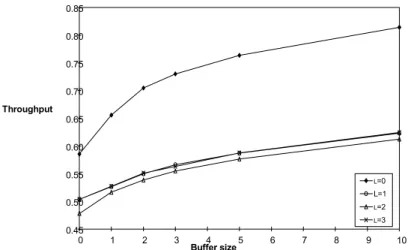
Our first finding is on the applicability of the famous "reversibility property" in considering S as a performance measure. Muth (1979) has proved that throughput (T) remains invariant if the items pass through the stations in the reverse order. This result called "the reversibility property" enables to reduce the search space significantly. However, our results on the interdeparture time variability indicate that the reversibility property does not hold for S (see Figure 1 and Figure 2 for a comparison). This has been also observed by Hendricks and McClain (1993). This means that the order of the stations in which items are processed is an important factor for S.
We also found that the interdeparture time variability increases as the number of stations (N) increases at a decreasing rate (Figure 2). This is simply due to the fact that more opportunities exist for the blockage and starvation events that result in higher S. This observation was previously made by Martin and Lau (1990) and Hendricks and McClain (1993). But additionally, we found that if there is a bottleneck station in the system, shifting the bottleneck station towards the end of the line (i.e., increasing L from 1 to 2 and to 3) reduces the effect of N on S (Figure2). The explanation of this new and important finding is as follows. Our simulation experiments indicated that one can identify two types of effects of a bottleneck station on S: Type-1 is the increasing effect on S due to the decrease in the number of units entering the system per unit time.This is due to the fact that the interdependency of the stations increases as fewer units enter the system. Type-2 is the decreasing effect on S due to the mitigation of the interference of the stations upstream and downstream of the bottleneck station (e.g., a bottleneck station in the middle of the line divides the entire line into two shorter lines). As can be seen in Figure 2, a bottleneck station at the beginning of the line increases S for any N due to mainly the Type-1 effect when compared to the non-bottleneck case. On the contrary, when the bottleneck station is at the end of the line (i.e., L=3), only Type-2 effect
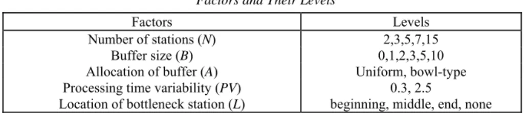
Average of ThRateBneck BufSizeL=0 L=1 L=2 L=3 00.5850270.5033820.4780540.503475 10.6553590.5266040.5162310.527002 20.7044290.5499410.5383640.550808 30.7300380.5659210.5547540.563124 5 0.763350.5871920.5765160.587516 100.8141130.6230230.6122940.624259 0.45 0.50 0.55 0.60 0.65 0.70 0.75 0.80 0.85 0 1 2 3 4 5 6 7 8 9 10 Buffer size Throughput L=0 L=1 L=2 L=3
Figure 1 Effects of Buffer size (B) and Location of Bottleneck (L) on Throughput (T)
exists and S is predominantly determined by the variability of the bottleneck station. Note that in Figure 2a, when L=3, S is solely determined by the variability of the bottleneck station, whereas in Figure 2b, the effect of the other stations still exist. When the bottleneck station is between the first and the last locations (i.e., in the middle), both Type-1 and Type-2 simultaneously determine the net effect on S. Hence, one should expect that the plot of the middle case to lie between the plots of bottleneck-at-the-beginning and bottleneck-at-the-end cases.
The implication of the above finding is as follows: if the existence of a bottleneck station is inevitable, then one should attempt to shift the location of the bottleneck station towards the end of the line.This can be accomplished by employing the relatively slower workers and/or assigning slower machines to the stations close to the end of the line. Note that if we consider throughput as the only performance measure, then the bowl phenomenon recommends the slower stations being located at both ends of the line (Hillier, et al. 1993). However, our finding on S suggests placing the bottleneck station only at the end of the line.
Another finding is about the effect of buffer size (B) on the interdeparture time variability; we observed that S improves as B increases. This has also been reported by Martin and Lau (1990) and Hendricks and McClain (1993). However, we further noted that the improving effect of B on S is magnified as N and the processing time variability (PV) increase (Figure 3). This is because the effect of assigning buffer capacity is greater in longer lines in which the frequency of coupling events is relatively higher. With the same reasoning, the extra buffer capacity yields a large reduction in S in the high PV case as compared to the low PV case. In addition, the effect of B on S is drastically reduced when there is a bottleneck station in the system. For example, as depicted in Figure 4a (low PV case), the effect of B on S is
almost negligible for B>1. This follows from the fact that the extra buffer capacity in Average of PV Bneck PV_LOW PV_HIGH NumStat L=0 L=1 L=2 L=3 L=0 L=1 L=2 L=3 2 0.332787 0.478808 0.301452 3.172742 3.233023 3.080792 3 0.350845 0.5642 0.4857 0.3049 3.510558 3.680047 3.607003 3.382198 5 0.358263 0.633285 0.562467 0.304523 4.442349 4.468132 4.365755 4.079815 7 0.364249 0.666547 0.605018 0.304677 4.814353 4.823552 4.825226 4.427066 15 0.375286 0.708009 0.677268 0.304863 5.646838 5.756337 5.713061 5.292885
(a) Low PV (b) High PV
3.00 3.50 4.00 4.50 5.00 5.50 6.00 2 4 6 8 10 12 14 16 Number of stations Interde
parture time std.dev
L=0 L=1 L=2 L=3 0.25 0.35 0.45 0.55 0.65 0.75 2 4 6 8 10 12 14 16 Number of stations Interde
parture time std.dev
L=0 L=1
L=2 L=3
Figure 2 Effects of Number of Stations (N) and the Location of Bottleneck Station (L) on the Interdeparture Time Variability (S)
the system cannot effectively utilized due to the bottleneck station. The extra buffer capacity assigned to the locations upstream of the bottleneck station stay full whereas the extra capacity in the locations downstream of the bottleneck station stay idle. In the high PV case, where we have more coupling between stations, the effect of B still exists and improves S (Figure 4b). The interaction between B and L is similar to the one observed between N and L; bottleneck-at-the-end case improves S for any B when compared to the nonbottleneck case (Figure 4).
We can summarize the above findings as follows: First, assigning extra buffer capacity improves S, but the improvement is relatively more significant in systems with a higher frequency of coupling events (e.g., longer lines, higher PV). Thus, the cost of assigning extra buffer capacity should be carefully compared with the benefit gained by the reduction in S. Since the amount of reduction in S can be very small (sometimes negligible) in short lines and/or low PV cases (see Figure 3a).
Average of PV NumStat PV_LOW PV_HIGH BufSize N=2 N=3 N=5 N=7 N=15 N=2 N=3 N=5 N=7 N=15 0 0.392703 0.45536 0.510088 0.537543 0.570528 3.288787 4.013913 4.942998 5.519653 7.381845 1 0.37386 0.428255 0.474894 0.493918 0.528416 3.262937 3.757508 4.540068 5.241434 6.305813 2 0.367827 0.42245 0.46114 0.482176 0.511326 3.117687 3.536805 4.359948 4.93828 5.923253 3 0.36679 0.41983 0.458193 0.478284 0.508625 3.17857 3.453533 4.457389 4.660105 5.557316 5 0.36455 0.41761 0.454691 0.47373 0.505603 3.15276 3.31831 4.294333 4.420924 5.035195 10 0.360363 0.414963 0.451528 0.471298 0.500728 2.972373 3.189643 3.741335 3.953453 4.300043
(a) Low PV (b) High PV
0.30 0.35 0.40 0.45 0.50 0.55 0.60 0 2 4 6 8 10 Buffer size Inter depar tur e time std.dev N=2 N=3 N=5 N=7 N=15 2.50 3.00 3.50 4.00 4.50 5.00 5.50 6.00 6.50 7.00 7.50 0 2 4 6 8 10 Buffer size Inter depar tur e time std.dev N=2 N=3 N=5 N=7 N=15
Figure 3 Effects of Buffer Size (B) and Number of Stations (N) on Interdeparture Time Variability (S) Average of PV Bneck PV_LOW PV_HIGH BufSize L=0 L=1 L=2 L=3 L=0 L=1 L=2 L=3 0 0.483176 0.607694 0.596483 0.32638 5.101386 5.05927 5.466538 4.926112 1 0.389546 0.635651 0.592863 0.3076 4.921436 4.996579 5.179396 4.739683 2 0.35251 0.630883 0.59454 0.300188 4.688735 4.75578 4.889391 4.436283 3 0.33968 0.63221 0.595656 0.299474 4.59691 4.571481 4.679459 4.330623 5 0.32529 0.632243 0.595979 0.300521 4.284998 4.396479 4.533306 3.943773 10 0.313185 0.632243 0.595329 0.29983 3.824398 3.993469 4.107067 3.292741
(a) Low PV (b) High PV
0.20 0.25 0.30 0.35 0.40 0.45 0.50 0.55 0.60 0.65 0 2 4 6 8 10 Buffer size In te rdepar tu re t im e st d. dev L=0 L=1 L=2 L=3 3.00 3.50 4.00 4.50 5.00 5.50 0 2 4 6 8 10 Buffer size In te rdepar tu re t im e st d. dev L=0 L=1 L=2 L=3
Figure 4 Effects of Buffer size (B) and Location of Bottleneck (L) on Interdeparture Time Variability (S)
Second, existence of a bottleneck station in the system reduces the positive effect of
B on S. Again, we find that the best location for the bottleneck station for any B is
the last location in the line.
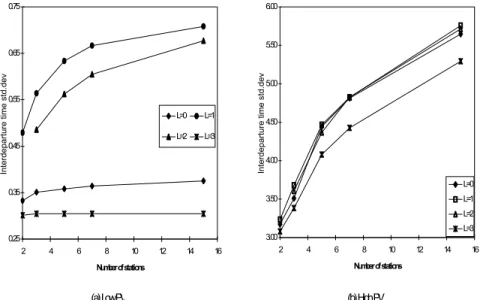
With respect to the allocation of buffer capacity (A), we made the following observations: First, as seen in Table 2, bowl type allocation has an improvement on
S only in the high PV case (t-test results showed that difference between the bowl
and uniform allocations are significant in the high PV case). Because the high PV causes more coupling between stations and the coupling of the middle stations becomes more critical. The reason for not observing an improvement in the low PV case can be attributed to our process of designing bowl allocation. In the literature, bowl phenomenon is generally created by smoothly adjusting the mean processing times of the stations. This usually results in very smooth bowl allocation. For example, in a study conducted by Pike and Martin (1994) to determine the optimal bowl configuration on lines up to 30 stations, it is found that the maximum and the minimum processing times are 1.076 and 0.981, respectively. On the contrary, in our
case, the bowl type allocation is achieved by adjusting the buffer capacities in discrete units (similar to Hillier and So, 1991). This generally results in a non-smooth (deep) bowl allocation, and consequently does not lead to an improvement on S.
Furthermore, as illustrated in Figures 5, bowl buffer allocation starts to reduce S significantly in the high PV case when N and L increase and B decreases (these results are also verified by t-tests). The above findings suggest that bowl type buffer capacity allocation plays an important role in reducing the interdeparture time variability only when the frequency of coupling events is relatively higher (i.e., higher processing time variability, longer lines, and smaller buffer capacities). Note also that the effect of the bowl allocation is considerably high when the location of the bottleneck is shifted towards the end of the line.
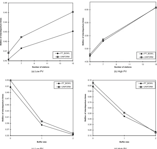
To obtain further insight of the behavior of the system, we have conducted additional experiments and examined the effects of the traditional bowl-phenomenon as suggested in the literature (Hillier and Boling, 1966). In the new experiments, we varied N (5, 7, and 15) and B (0, 1, and 2), and created the bowl-phenomenon by adjusting the mean of processing times as recommended by Pike and Martin (1994). As depicted in Figure 6, the results show that the traditional bowl improves S and this effect is magnified for large N and small B in the low PV case. We also note that the traditional bowl improves T but increases Q (even though this increase was not significant at = 0.05). Thus, we can conclude that the bowl-phenomenon (both the traditional approach and the one created by buffer capacities) has a positive effect on
S.
We have already discussed the effects of PV on the interdeparture time variability (S) and found that high PV causes S to deteriorate in all its two-way interactions with
Table 2
Effects of Buffer Allocation (A) on Interdeparture Time Variability (S)
Interdeparture time standard deviation Processing time variability Bowl Uniform
Low 0.4841 0.4832
High 4.7598 4.8041
the other factors (Figure 7). We also noted that the inverted bowl obtained by having the bottleneck station in the middle of the line deteriorates S drastically in the high
PV case (Figure 7a and 7b). The same behavior is also valid for throughput (Figure
7c and 7d). In other words, the inverted bowl decreases throughput only in the high
(a) Low PV (b) High PV
(c) Low PV (d) High PV
(e) Low PV (f) High PV
0.45 0.46 0.47 0.48 0.49 0.50 0.51 0.52 5 7 9 11 13 15 Number of stations In te rdepart ure tim e st d. dev BOWL UNIFORM 4.00 4.20 4.40 4.60 4.80 5.00 5.20 5.40 5.60 5 7 9 11 13 15 Number of stations In te rdepart ure tim e st d. dev BOWL UNIFORM 0.30 0.35 0.40 0.45 0.50 0.55 0.60 0.65 0.70 0 1 2 3 Location of bottleneck In te rd ep ar tu re tim e s td .d ev BOWL UNIFORM 4.40 4.50 4.60 4.70 4.80 4.90 5.00 0 1 2 3 Location of bottleneck In te rdepart ure tim e st d. dev BOWL UNIFORM 0.47 0.48 0.48 0.49 0.49 0.50 0.50 0.51 0 2 4 6 8 10 Buffer size In te rdepart ure tim e st d. dev BOWL UNIFORM 3.80 4.00 4.20 4.40 4.60 4.80 5.00 5.20 5.40 5.60 0 2 4 6 8 10 Buffer size In te rdepart ure tim e st d. dev BOWL UNIFORM
Figure 5 Effects of Number of Stations (N), Location of Bottleneck (L), Buffer Size (B), and Buffer Allocation (A) on Interdeparture Time Variability (S)
(a) Low PV (b) High PV (c) Low PV (d) High PV 4.50 5.00 5.50 6.00 6.50 5 7 9 11 13 15 Number of stations S tdDev of inter d epar tur e tim es PT_BOWL UNIFORM 0.40 0.41 0.42 0.43 0.44 0.45 0.46 5 7 9 11 13 15 Number of stations S tdDev of inter d epar tur e tim es PT_BOWL UNIFORM 5.10 5.20 5.30 5.40 5.50 5.60 5.70 5.80 5.90 6.00 6.10 0 1 2 Buffer size S tdD ev of inter depar tur e ti m e s PT_BOWL UNIFORM 0.35 0.37 0.39 0.41 0.43 0.45 0.47 0.49 0.51 0.53 0 1 2 Buffer size S tdD ev of inter depar tur e ti m e s PT_BOWL UNIFORM
Figure 6 Effects of Number of Stations (N), Buffer Size (B), and Bowl-Phenomenon created by adjusting the processing time averages on interdeparture time variability (S)
4.2 Results on the Average and Variance of WIP Inventory
Our first finding on the average WIP inventory (Q) is that it increases as N increases. As depicted in Figure 8a, this increase is almost linear especially for large N. The explanation of this observation can be directly made from Little's formula (Q = T * Lead time); increasing N leads to a linear increase in lead time while the decrease in
T becomes insignificant after a certain value of N. Hence, the increase in Q as N
increases stays linear.
The above finding on the average WIP inventory is an important one. Because the effect of N on Q does not terminate as N increases. Whereas as noted before, the effect of N on both S and T decreases (it becomes almost insignificant beyond a certain value of N). Thus, one should consider the level of Q as the major controlling factor when determining the number of stations to be used in the system.
In contrast to the throughput measure, the relationship between L and Q are strong. Q increases as the bottleneck station shifts towards the end of the line, since the
Average of PV
Bneck PV_LOW PV_HIGH 0 0.359502 4.534194 1 0.629873 4.600148 2 0.595038 4.758628 3 0.304284 4.235008
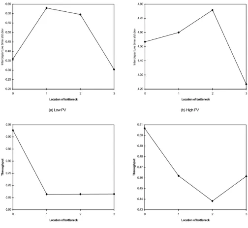
(a) Low PV (b) High PV
Average of PV
Bneck PV_LOW PV_HIGH 0 0.927241 0.50669 1 0.664186 0.461963 2 0.664334 0.438196 3 0.664634 0.461546 (c) Low PV (d) High PV 0.20 0.25 0.30 0.35 0.40 0.45 0.50 0.55 0.60 0.65 0 1 2 3 Location of bottleneck In te rd e p a rtu re tim e s td .d e v 4.20 4.30 4.40 4.50 4.60 4.70 4.80 0 1 2 3 Location of bottleneck In te rd e p a rtu re tim e s td .d e v 0.60 0.65 0.70 0.75 0.80 0.85 0.90 0.95 0 1 2 3 Location of bottleneck Thr oughput 0.43 0.44 0.45 0.46 0.47 0.48 0.49 0.50 0.51 0 1 2 3 Location of bottleneck Thr oughput
Figure 7 Effects of Location of Bottleneck (L) on Interdeparture Time Variability (S) and Throughput (T)
buffer capacities upstream of the bottleneck station stay full. The implication of this finding is also important, because it conflicts with the earlier suggestion that shifting the location of the bottleneck station towards the end of the line is desirable for S. Hence, the decision to locate the bottleneck station in the line should be made in practice with respect to the relative importance of S and Q measures.
Our simulation experiments also indicated that buffer allocation has a significant impact on the average WIP. As can be intuitively expected, bowl-type allocation resulted in higher average WIP inventory compared to the uniform-type allocation.
Our last finding on the average WIP inventory is that increasing B has a negative effect on Q up to a certain level, because the excessive amount of buffer capacity between the stations stay unutilized (Figure 8b). Recall that increasing B improves S and T at a decreasing rate (see Figure 5 and Figure 9). We also note that the effect of increasing B on Q exists for a much larger range when compared with the effect on S
and T. Combining the above findings, we can conclude that the benefits gained from assigning buffer capacity becomes minimal after a certain value of B. Hence, the decision to set the amount of buffer capacity should be made cautiously, since the associated cost figures can be of a significant size.
Finally, we have conducted additional experiments to examine the effects of the design factors (N, L, PV, and B) on the variability of WIP inventory. Both the variance and CV of WIP inventory are measured in the experiments. The variance (or CV) is important to construct a confidence interval on the average WIP. Because, this additional information can be utilized by designers to set the upper limits on buffer capacities (i.e., buffer capacities can be set to lower values if the design results in a smaller variance).
As depicted in Figure 10, the variance of WIP increases as the buffer size increases. This is especially observed in the high PV case with longer line lengths Average of Buflev NumStat Total 2 1.75128 3 3.499427 5 7.69325 7 11.27192 15 26.69205 (a) (b) 0.00 5.00 10.00 15.00 20.00 25.00 30.00 1 3 5 7 9 11 13 15 Number of stations Average WI P in ventory 0.00 10.00 20.00 30.00 40.00 50.00 60.00 0 10 20 30 40 50 60 70 80 90 100 Buffer size Average WI P in ventory
Figure 8 Effects of Number of Stations (N) and Buffer size (B) on Average WIP Inventory (Q)
Average of PV
BufSize PV_LOW PV_HIGH Average of NumStat
0 0.682745 0.356375 BufSize N=2 N=3 N=5 N=7 N=15 1 0.720552 0.394631 0 0.627478 0.5549 0.508089 0.485416 0.448895 2 0.736302 0.438535 1 0.668037 0.605433 0.560752 0.539093 0.507593 3 0.741119 0.468942 2 0.686832 0.629419 0.591724 0.571158 0.541093 5 0.745417 0.515233 3 0.695362 0.644798 0.608615 0.592445 0.560273 10 0.748856 0.59161 5 0.711447 0.664275 0.632563 0.61836 0.592656 10 0.735967 0.693743 0.673365 0.658533 0.642396 (a) (b) 0.30 0.35 0.40 0.45 0.50 0.55 0.60 0.65 0.70 0.75 0.80 0 2 4 6 8 10 Buffer size Thr oughput PV_LOW PV_HIGH 0.40 0.45 0.50 0.55 0.60 0.65 0.70 0.75 0 2 4 6 8 10 Buffer size Thr oughput N=2 N=3 N=5 N=7 N=15
Figure 9 Effects of Buffer Size (B), Processing Time Variability (PV), and Number of Stations (N) on Throughput (T)
(a) Low PV (b) Low PV
(c) High PV (d) High PV 0.35 0.40 0.45 0.50 0.55 0.60 0.65 0.70 0.75 0 1 2 3 4 5 6 7 8 9 10 Buffer size C V of W IP invent o ry N=3(Uniform) N=7(Bowl) N=7(Uniform) 0.35 0.45 0.55 0.65 0.75 0.85 0.95 1.05 1.15 0 1 2 3 4 5 6 7 8 9 10 Buffer size C V of W IP invent o ry N=3(Uniform) N=7(Bowl) N=7(Uniform) 0 20 40 60 80 100 120 140 0 1 2 3 4 5 6 7 8 9 10 Buffer size Var ian ce o f W IP in ven to ry N=3(Uniform) N=7(Bowl) N=7(Uniform) 0 1 2 3 4 5 6 7 8 0 1 2 3 4 5 6 7 8 9 10 Buffer size Var ian ce o f W IP in ven to ry N=3(Uniform) N=7(Bowl) N=7(Uniform)
Figure 10 Effects of Buffer Sizes (B), Processing Time Variability (PV), and Number of Stations (N) on Variance and CV of WIP Inventory
and bowl-type buffer allocation. This counter-intuitive result (i.e.,observing a deterioration in the system performance even though the available resource is increased) is due to the fact that WIP can fluctuate in a wider range of buffer capacity. On the contrary, however, we also noted that CV of WIP decreases as B increases due to the much larger increase in the average WIP. The above findings support our previous conclusions and suggest that designers should not increase B beyond a certain limit.
We also studied the effect of L on the variance (and CV) of WIP. Since, according to our previous results, PV plays an important role in describing the effect of the bottleneck station, we analyzed the high and low PV cases separately. As illustrated in Figure 11a, in the low PV case, the existence of a bottleneck station improves the variance of WIP. This is due to the fact that buffers upstream of the bottleneck station stay full whereas the buffers downstream of the bottleneck station stay empty. This leads to a lower variance compared to the nonbottleneck case. Examining the effect of L on the CV of WIP (Figure 11b) reveals that as the level of
L increases, the CV decreases except for L=1. In this exception case, the average of
WIP is considerably smaller than the level in the nonbottleneck case that results in the higher CV. For the other locations of the bottleneck station, the average WIP increases with smaller variance; hence, the net effect reduces the value of CV. Similar to the low PV case, the same pattern of CV has been observed in the high PV case (Figure 11d). However, we noted an unexpected behavior of the variance of WIP for the L=2 level in the high PV case. As illustrated in Figure 11c, the variance of WIP decreases only when the bottleneck station is at the middle of the line. This situation arises because the L=2 level divides the entire line into two shorter lines which leads to smaller variances (recall that increasing N has an increasing effect on the variance of WIP in the high PV case). Note also that the negative effect of bowl allocation is observed only in the high PV case.
A summary of the factor effects on the performance measures is given in Appendix A. The diagonal entries in this table show the main factor effects, whereas the other entries depict the two-way interaction effects. The results are also analyzed by ANOVA for statistical significance (see Table 3). In general, test results confirmed our findings reported in the paper.
(a) Low PV (b) Low PV (c) High PV (d) High PV 0.30 0.40 0.50 0.60 0.70 0.80 0.90 1.00 0 1 2 3 Location of bottleneck CV of W IP invent o ry N=3(Uniform) N=7(Bowl) N=7(Uniform) 0.00 0.50 1.00 1.50 2.00 2.50 3.00 3.50 4.00 0 1 2 3 Location of bottleneck CV of W IP invent o ry N=3(Uniform) N=7(Bowl) N=7(Uniform) 5 10 15 20 25 30 35 40 45 50 0 1 2 3 Location of bottleneck V ar ian ce o f W IP in ven to ry N=3(Uniform) N=7(Bowl) N=7(Uniform) 0 2 4 6 8 10 12 0 1 2 3 Location of bottleneck V ar ian ce o f W IP in ven to ry N=3(Uniform) N=7(Bowl) N=7(Uniform)
Figure 11 Effects of Location of Bottleneck (L), Processing Time Variability (PV), and Number of Stations (N) on Variance and CV of WIP Inventory
Table 3 Anova test results
Source DF F Value Pr > F Significant
Dependent Variable: Throughput (T)
PV 1 99999.99 .0001 Yes N 4 10465.02 .0001 Yes A 1 1043.96 .0001 Yes B 5 12249.99 .0001 Yes L 3 46377.38 .0001 Yes N*A 2 317.69 .0001 Yes N*B 20 397.19 .0001 Yes N*L 11 0.00 1.0000 No A*B 4 1161.96 .0001 Yes A*L 3 86.47 .0001 Yes B*L 15 403.70 .0001 Yes PV*N 4 6375.31 .0001 Yes PV*A 1 1041.59 .0001 Yes PV*B 5 5181.65 .0001 Yes
PV*L 3 20894.76 .0001 Yes
Dependent Variable: Std.Dev of Interdeparture Times (S)
PV 1 53274.33 .0001 Yes N 4 571.13 .0001 Yes A 1 107.98 .0001 Yes B 5 123.65 .0001 Yes L 3 107.36 .0001 Yes N*A 2 0.00 1.0000 No N*B 20 18.86 .0001 Yes N*L 11 0.00 1.0000 No A*B 4 23.17 .0001 Yes A*L 3 1.30 .2719 No B*L 15 1.53 .0873 No PV*N 4 462.71 .0001 Yes PV*A 1 82.06 .0001 Yes PV*B 5 111.69 .0001 Yes PV*L 3 13.16 .0001 Yes
Dependent Variable: Average WIP inventory (Q)
PV 1 4.89 .0270 Yes N 4 41013.25 .0001 Yes A 1 21504.13 .0001 Yes B 5 45111.15 .0001 Yes L 3 16749.98 .0001 Yes N*A 2 0.00 1.0000 No N*B 20 5282.47 .0001 Yes N*L 11 1965.11 .0001 Yes A*B 4 0.00 1.0000 No A*L 3 1285.52 .0001 Yes B*L 15 2909.05 .0001 Yes PV*N 4 1.31 .2621 No PV*A 1 1.12 .2891 No PV*B 5 8.53 .0001 Yes PV*L 3 7948.58 .0001 Yes
5. Discussion and Suggestions for Further Research
In this paper, we studied the unpaced and asynchronous serial production lines with reliable machines. Specifically, we analyzed the problem for the interdeparture time variability and average WIP inventory measures. Based on our simulation experiments and statistical analysis of the results, we have obtained several new findings about the effect of various system design parameters on the interdeparture time variability and average WIP inventory. We have also confirmed some of the results reported earlier in the literature. These new findings and the related managerial implications are summarized as follows:
1. Similar to the throughput measure, increasing the line length deteriorates the interdeparture time variability at a decreasing rate. This effect is more noticeable in systems with higher processing time variability. When there is a bottleneck station in the system, shifting it towards the end of the line reduces the effect of line length on the interdeparture time variability.
2. The location of the bottleneck station plays an important role for the interdeparture time variability. Results of the experiments indicated that the interdeparture time variance changes from the highest value (when the bottleneck is the first station in the line) to the lowest value (when the bottleneck is the last station in the line). Moreover, the interdeparture time variability associated with the non-bottleneck case is found to be between these two extreme values. In contrast to the throughput case, this new finding suggests that a carefully selected location for the bottleneck station can indeed improve the interdeparture time variability when compared to the non-bottleneck case. In our study, we also found that the location of the non-bottleneck station affects throughput in the high processing time variability case. Hence, by considering both throughput and interdeparture time variability, we suggest to locate the bottleneck station towards the end of the line.
3. Even though shifting the location of the bottleneck station towards the end of the line minimizes the interdeparture time variability (recall that it has no effect on throughput for the low PV case), it is not desirable for the average WIP inventory measure since more items tend to accumulate in the buffers upstream of the bottleneck station. Thus, one should consider a tradeoff between the interdeparture time variability and WIP inventory in locating the bottleneck station. Our results also indicated that the bottleneck station should be located in the middle of the line when considering the variance of WIP. 4. A similar tradeoff exists between the performance measures (S, T, Q, and
variability of WIP) when the number of stations is considered. Unlike the interdeparture time variability and throughput, the effect of the number of stations on the average and variance of WIP inventory does not terminate as the number of stations increases. Also, unlike the other performance measures,
CV of WIP decreases as the line length increases. Thus, a system designer
should find a compromise between the above performance measures in setting the optimal line length.
5. We found that assigning extra buffer capacity improves the interdeparture time variability. This effect is more prominent in systems with higher processing time variability and number of stations. However, the existence of a bottleneck station reduces this improving effect drastically. In contrast to throughput and interdeparture time variability, buffer capacity has a negative effect on the average and variance of WIP, but not on the CV of WIP inventory. Also, the effect of buffer capacity on the average WIP inventory exists for a much larger range when compared to the effect on throughput and interdeparture time variability. Since the effect of buffer capacity on various performance measures are different and there is a cost associated with assigning extra buffer capacity, system designers should determine the level of buffer capacity cautiously.
6. Similar to the throughput measure, bowl-phenomenon has a positive effect on the interdeparture time variability. This effect is noticeable in both the traditional approach and the one created by buffer capacities in this paper. Unlike the other performance measures, bowl phenomenon deteriorates both
the variance and CV of WIP. Hence, this downside effect should be measured against the benefits of the bowl phenomenon.
The above results should be interpreted with reference to the assumptions of the model and experimental conditions specified in this paper. Hence, there is a need for further research to study the problem under different system characteristics and experimental conditions (e.g., synchronous lines, unreliable machines, imperfect yield rates, etc.). More in-depth analysis on the tradeoff situations stated above should also be pursued by researchers to increase applicability of the findings.
6. References
1. Anderson DR and Moodie CL (1969). Optimal buffer storage capacity in production line systems. International Journal of Production Research 7: 233-240.
2. Baker KR Powell SG and Pyke DF (1994). A predictive model for the throughput of unbalanced, unbuffered three-station serial lines. IIE
Transactions 26: 62- 71.
3. Blumenfeld DE (1990). A simple formula for estimating throughput of serial production lines with variable processing times and limited buffer capacity.
International Journal of Production Research 28: 1163-1182.
4. Chow WM (1987). Buffer capacity analysis for sequential production lines with variable process times. International Journal of Production Research 25: 1183-1196.
5. Conway R Maxwell W McClain JO and Thomas LJ (1988). The role of work-in-process inventory in serial production lines. Operations Research 36: 229-241.
6. Dallery Y and Gershwin SB (1992). Manufacturing flow line systems: a review of models and analytical results. Queueing Systems 12: 3-94.
7. Dar-El EZ and Mazer A (1989). Predicting the performance of unpaced assembly lines where one station variability may be smaller than the others.
International Journal of Production Research 27: 2105-2116.
8. Hendricks KB (1992). The output processes of serial production lines of exponential machines with finite buffers. Operations Research 40: 1139-1147. 9. Hendricks KB and McClain JO (1993). The output processes of serial production lines of general machines with finite buffers. Management Science 39: 1194-1201.
10. Hillier FS and Boling R (1966). The effect of some design factors on the efficiency of production lines with variable operation times. Journal of
Industrial Engineering 17: 651-658.
11. Hillier FS and Boling R (1967). Finite queues in series with exponential or Erlang service times - A numerical approach. Operations Research 15: 286-303.
12. Hillier FS and Boling R (1979). On the optimal allocation of work in symmetrically unbalanced production line systems with variable operation times. Management Science 25: 721-728.
13. Hillier FS and So KC (1991). The effect of the coefficient of variation of operation times on the allocation of storage space in production line systems.
IIE Transactions 23: 198-206.
14. Hillier FS and So KC (1993). Some data for applying the bowl phenomenon to large production line systems. International Journal of Production Research 31: 811-822.
15. Hillier FS So KC and Boling RW (1993). Toward characterizing the optimal allocation of storage space in production line systems with variable processing times. Management Science 39: 126-133.
16. Knott K and Sury RJ (1987). A study of work-time distributions on unpaced tasks. IIE Transactions 19: 50-55.
17. Liu CM Su SF and Lin CL (1996). Predictive models for performance evaluation of serial production lines. International Journal of Production
Research 34: 1279-1291.
18. Martin GE (1993). Predictive formulae for unpaced line efficiency.
International Journal of Production Research 31: 1981-1990.
19. Martin GE and Lau HS (1990). Dynamics of the output interval distribution in unpaced lines. Computers and Industrial Engineering 18: 391-399.
20. Miltenburg GJ (1987). Variance of the number of units produced on a transfer line with buffer inventories during a period of length T. Naval Research
Logistics 34: 811-822.
21. Muth EJ (1973). The production rate of a series of work stations with variable service times. International Journal of Production Research 11: 155-169. 22. Muth EJ (1979). The reversibility property of production lines. Management
Science 25: 152-158.
23. Muth EJ and Alkaff A (1987). The throughput rate of three-station production lines: a unifying approach. International Journal of Production Research 25: 1405-1413.
24. Pegden CD Shannon RE and Sadowski RP (1995) Introduction to simulation
using SIMAN. 2nd edition. McGraw-Hill: New York.
25. Pike R and Martin GE (1994). The bowl phenomenon in unpaced lines.
International Journal of Production Research 32: 483-499.
26. Powell SG (1994). Buffer allocation in unbalanced three-station serial lines.
International Journal of Production Research 32: 2201-2217.
27. Rao NP (1975). On the mean production rate of a two-stage production system of the tandem type. International Journal of Production Research 13: 207-217.
28. Rao NP (1975). Two-stage production systems with intermediate storage. AIIE
Appendix A
Summary of the findings
Summary of the Factor Effects on the Performance Measures
Effect of the factors on S
N B L PV A
N
Increasing effect at a decreasing rate Decreasing effect of B is pronounced for large N Decreasing effect of L is pronounced for large N In the high PV case, the increasing effect of N is more prominent No significant effect is observed B Decreasing effect at a decreasing rate Decreasing effect of B is pronounced for L=3 Decreasing effect of B is pronounced for high PV Uniform allocation yields lower S for all B values considered L Decreasing effect as L is increased
For low PV, the improving effect of increasing L is pronounced No significant effect is observed PV Strong increasing effect In the high PV case, bowl allocation has a decreasing effect A Uniform allocation yields lower S
Effect of the factors on Q N
An almost linear relationship exists Increasing effect of B is pronounced at higher N For L greater than 1, the increase in Q is pronounced No significant effect is observed No significant effect is observed B Increasing B up to a certain value has an increasing effect For L greater than 1, the increase in Q is pronounced No significant effect is observed No significant effect is observed L Strong increasing effect
For low PV, the increase in Q as L is increased is pronounced
Uniform allocation yields lower Q for all L values PV High PV yields slightly higher Q No significant effect is observed A Uniform allocation yields lower Q
Effect of the factors on T
N B L PV A
N
Inversely proportional effect at a decreasing rate
Increasing effect of B is pronounced in longer lines No significant effect is observed In the high PV case, the decreasing effect of N intensifies Bowl allocation yields higher T for all N considered B Increasing effect at a decreasing rate For L greater than or equal to 0, the effect of B is significantly reduced In the high PV case, the increasing effect of B intensifies Uniform allocation yields higher T for all B considered L Having a bottleneck station significantly reduces T For high PV, L = 2 has a decreasing effect For L=0, uniform allocation yields higher T PV Strong decreasing effect Uniform allocation results in higher T for high PV A Uniform allocation yields slightly higher T
Effect of the factors on the variability of WIP N
Increasing effect on the variance
Effects of B on the variance and CV are pronounced at higher N
(not measured) (not measured) (not measured)
B Increasing effect on the variance and decreasing effect on the CV (not measured) Effects of B on the variance and CV are pronounced at high PV Effects of B on the variance and CV are pronounced at bowl-type buffer allocation L Decreasing effect on CV except for L=1 Effect on CV is magnified at high PV (not measured) PV Increasing effect
on the variance (not measured)
A Bowl allocation
deteriorates both the variance and CV