Analyses of serial production lines and assembly systems for throughput and inyerdeparture time variability

(1)

.0 ;*ί '‘ . g л ^ t í t sr}i^ />·« ■_»; p ‘y, ■.?: ;’-· ;'^ “ V' ] X '^ ' ' . ¡ 1 vj • - . ^·· „у ... .ν' . J V --'^ /J _{.i. -}1 _S-J_{X i} А? Í5j". 'à i < -'6 «I r äi# 4.^ » .«ií' L^·· ' / .^1 w ifii ¿J 'ü J ' f ^ i l T r!; 4;) 5 1 ч 7 iC j1* Йy ^' й i*· ., | і ' | » ' | 7 ‘^ ,.¿ ¿ b :¡ y ¡ t J «>'« WA 4ГГ» ^ ■> >■;,·; í .* í i í M Щ 4w>¿ уОй l ,'. Xp. Ч ■ ;· _{■·.*) Ί·;} -i 'i ki 4t 'i 41 W •‘Τ' ·4 4 -3 ,·: ·^ VjUf *νν ■ α,ί^ ' 1 Ί W . ί - Î i "i ■· 4^ 4» чО» ύ Vbl J W Μ ύΧΜ$ήϊΤζΈύ ΎΖ 'ГгН ^-£РЛ?ГГлл£>57 Or ^7ï?^· ^ν··χ ■"‘' T'i^-rr - v , V >««:* w - w _ 4 ^ . .Г ' ^ 7 ^ · . ѵ ^ Ь і ^ Ь в ^Ш іС п a f ¿k K £ íJ7 İ--07, í;·:·''

(2)

TIME VARIABILITY

A THESIS

SUBMITTED TO THE DEPARTMENT OF INDUSTRIAL ENGINEERING AND THE INSTITUTE OF ENGINEERING AND

SCIENCE OF BiLKENT UNIVERSITY

IN PARTIAL FULFILLMENT OF THE REQUIREMENTS

FOR THE DEGREE OF

MASTER OF SCIENCE

By

Abdullah Gürhan Kök June, 1998

(3)

TS

İST. t

■

i ^ 3 s

(4)

Assoc. Prof İhsan Sabuncuoğlu (Principal Advisor)

I certify that I have read this thesis and that in my opinion it is fully adequate, in scope and in quality, as a thesis for the degree of Master of Science.

Assoc. Prof Cemal Dinçer

I certify that I have read this thesis and that in my opinion it is fully adequate, in scope and in quality, as a thesis for the degree of Master of Science.

Assoc. Prof Erdal Erel

Approved for the Institute of Engineering and Science:

C*

Prof Mehmet Baray

Director of Institute of Engineering and Science a r a y ^ y

(5)

ABSTRACT

ANALYSES OF SERIAL PRODUCTION LINES

AND ASSEMBLY SYSTEMS FOR THROUGHPUT

AND INTERDEPARTURE TIME VARIABILITY

Abdullah Gürhan Kök M .S. in Industrial Engineering Advisor: A ssoc. Prof. İhsan Sabuncuoğlu

June, 1998

In this thesis, we study three different but closely related production system design problems. First, we investigate the effects of various design factors such as number of stations, buffer capacity, allocation of bulfers and location of a bottleneck on the interdeparture time variability of serial production lines. In the second part, we study the effects of number of component stations, processing time distributions, buffers and buffer allocation schemes on throughput and interdeparture time variability of assembly systems. As an alternative to work transfer, we introduce variability transfer and assess its effectiveness. We analyze the anomaly displayed by optimal throughput for some processing time distributions and uncover the underlying details of this behavior. In the third part, we analyze serial production lines and assembly systems under constant workload condition. In addition to investigating the problem of determining the optimal system size, we examine the effects of other design factors such as buffers and material handling time on throughput, interdeparture time variability and cost related measures. Each part reveals several important findings. We also discuss the managerial implications of these findings to present guidelines for the practitioners.

Keywords: Throughput, Interdeparture Time Variability, Serial Production Lines,

Assembly Systems, Performance Evaluation.

(6)

SİSTEMLERİNİN ÜRETİM HIZI VE ÜRÜN ÇIKIŞ

ZAMANI FARKLARININ VARYANSI AÇISINDAN

İNCELENMESİ

Abdullah Gürhan Kök

Endüstri M ühendisliği, Yüksek Lisans Danışman: D oç. Dr. İhsan Sabuncııoğlıı

June 1998

Bu çalışmada üretim sistemi tasarım problemleri incelenmiştir. İlk olarak, seri üretim hatlarında istasyon sayısı, stok kapasitesi, stok tahsis biçimleri ve darboğaz istasyonun konumu gibi bir çok dizayn faktörünün ürün çıkış zamanı farklarının varyansı açısından performansı üzerindeki etkileri analiz edilmiştir. Çalışmanın ikinci kısmında, montaj sistemlerindeki parça istasyonu sayısı, işlem zamanı dağılımları, stok kapasitesi ve stok tahsis biçimleri gibi faktörlerin üretim hızı ve ürün çıkış zamanı farklarının varyansma etkileri incelenmiştir. İş transferine alternatif olarak değişkenlik transferi sunulmuş ve etkinliği değerlendirilmiştir. Daha önceki araştırmalar optimal üretim hızının bazı işlem zamanı dağılımları için anormal bir davranış sergilemekte olduğunu göstermiştir. Bu olgu derinlemesine incelenmiş ve sebepleri açıklanmıştır. Üçüncü kısımda ise, seri üretim hatları ve montaj sistemleri sabit iş yükü koşulu altında araştırılmıştır. Optimal sistem büyüklüğünün belirlenmesi probleminin yanı sıra bazı dizayn faktörlerinin üretim hızı, ürün çıkış zamanı farklarının varyansı ve maliyet ile ilgili ölçütler üzerine etkileri de çözümlenmiştir. Her aşamada bir çok yeni bulgu ve önemli pratik çıkarımlar da sunulmaktadır.

Anahtar sözcükler·. Üretim Hızı, Ürün Çıkış Zamanı Farklarının Varyansı, Seri

Üretim Hatları, Montaj Sistemleri, Performans Değerlendirilmesi.

(7)

(8)

I would like to express my deep gratitude to Dr. İhsan Sabuncuoğlu and Dr. Erdal Erel who supervised and encouraged me through all the stages of my study with

wholehearted kindness and sincerity. Without their guidance, this thesis would not be

possible.

I am also indebted to Dr. Cemal Dinçer for showing keen interest to the subject mat ter and accepting to read and review this thesis.

I would also like to thank to my office mates Eylem Tekin and Bahar Deler, my home

mate Savaş Arslan, my bridge partner Sinan Tathcıoğlu, Murat Temizsoy, Erdem Ofli,

Ayşin Oktay, Bekir Arslan, Ersin Keçecioğlu, Armağan Yavuz and Hakan Özaktaş for their help and friendship during my master study.

My special thanks go to my dearest parents and beloved sister and brother for their

morale support throughout my studies.

(9)

List of Figures

Figure 2.1 Schematic Viewofa Serial Production Lin e...9

Figure 2.2 Effectsof Buffer Size (B) and Locationof Bottleneck (L) on

Throughput... 12

Figure 2.3 Effectsof Numberof Stations (N) and Locationof Bottleneck

(L) ON Interdeparture Time Variability... 14

Figure 2.4 Effectsof Buffer Size (B) and Numberof Stations (N) on

Interdeparture Time Variability... 15

Figure 2.5 Effectsof Buffer Size (B) and Locationof Bottleneck (L) on

Interdeparture Time Variability... 16

Figure 2.6 Effectsof Numberof Stations (N), Locationof Bottleneck (L),

Buffer Size (B), and Buffer Allocation (A) on Interdeparture

Time Variability... 17

Figure 2.7 Effectsof Numberof Stations (N), Buffer Size (B), and Bowl-

Phenomenon Createdby Adjustingthe Mean Processing Times

ON Interdeparture Time Variability... 18

Figure 2.8 Effectsof Locationof Bottleneck (L) on Interdeparture Time

Variabilityand Throughput... 19

Figure 2.9 Effectsof Numberof Stations (N) and Buffer Size (B) on

AverageWIP Inventory...20

Figure 2.1 OEffectsof Buffer Size (B), Processing Time Variability (PV)

AND Numberof Stations (N) on Throughput...21

Figure 2.11 Effectsof Locationof Bottleneck (L), Processing Time '

Variability(PV), and Numberof Stations (N) on Varianceand

CV OF WIP Inventory... 23

Figure 2. 12Effectsof Locationof Bottleneck (L), Processing Time

Variability(PV), and Numberof Stations (N) on Varianceand

CV ofWIP Inventory...24

Figure 3.1 Schematic Viewofan Assembly System... 31

(12)

Figure 3.2 Effectof Parallelism (N) on Throughputin Balanced Casefor

Lognormal Processing Timeswith CV = 0.289...33

Figure 3.3 Effectof WT/C V/- on Throughput...35

Figure 3.4 Effectof WT/PV/- on Throughputfor Lognormal Processing

Tim es... 36

Figure 3.5 Effectof VT/-/- on Throughputfor Lognormal Processing Times

... 36

Figure 3.6 Effectof Parallelism (N) on Interdeparture Time Variabilityin

Balanced Casefor Lognormal Processing Timeswith CV =

0 .2 8 9 ... 37

Figure 3.7 Effectof WT/CV/- on Interdeparture Time Variability... 39

Figure 3.8 Effectof WT/CV/- on Interdeparture Time Variabilityandits

Componentsfor Lognormal Processing Times... 40

Figure 3.9 Effectof WT/PV/- on Interdeparture Time Variabilityfor

Lognormal Processing Tim e s... 41

Figure 3.1 OEffectof VT/-/- on Interdeparture Time Variabilityfor

Figure 3.11 Effectof WT/CV/T on Throughput... 45

Figure 3.12Effectof WT/CV/IDTV on Throughput... 46

Figure 3.13 Effectof Numberof Component Stationson Throughputand

Interdeparture Time Variabilityin Balanced Casefor

Figure 3 .14EFFECT of WT/CV/- on Throughputand Interdeparture Time

Variabilityfor Buffer Size = 1 and Lognormal Processing

Timeswith CV = 0 .6 ...49

Figure 3.15 Effectsof WT/CV/T on Throughputand WT/CV/IDTV on

Interdeparture Time Variabilityfor Buffer Size = 1 and

Lognormal Processing Timeswith CV = 0 .6 ... .■... 50

Figure 4.1 Schematic Viewofa Serial Production Lin e... 54

Figure 4.2 Schematic Viewofan Assembly System... 55

Figure 4.3 Effectof Numberof Stations (N) on Throughputand

Interdeparture Time Variabilityof Unbuffered Serial Lines

(13)

LIST OF FIGURES XI

Figure 4.4 Effectof Numberof Stations (N) on Throughputand

Interdeparture Time Variabilityof Unbuffered Assembly

Systems (Constant C V )... 58

Figure 4.5 Effectof Numberof Stations (N) on Throughputof Serial Lines

...59

Figure 4.6 Effectof Material Handling Time (MHT) on Throughputof

Serial Lines...61

Figure 4.7 Effectof Numberof Stations (N) on Throughputof Assembly

Systems...62

Figure4.8 Effectof Material Handling Time(MHT) on Throughputof

Assembly System s... 63

Figure 4.9 Effectof Numberof Stations (N) on Interdeparture Time

Variabilityof Serial Lin e s... 64

Figure4.10 Effectof Material Handling Time(MHT) on Interdeparture

Time Variabilityof Serial Lines... 65

Figure 4.11 Effectof Numberof Stations (N) on Interdeparture Time

Variabilityof Assembly Systems...66

Figure4. 12Effectof Material Handling Time(MHT) on Interdeparture

Time Variabilityof Assembly Systems... 67

Figure 4.13 Effectof System Size (N) on Cost (TC) and Profit (TP) of

Unbuffered Serial Lin e s...69

Figure 4.14 Effectof System Size (N) on Cost(TC) and Profit(TP) of

Unbuffered Assembly Systems... 70

Figure 4.15Effectof Imperfect Yield Rateand Unreliable Stationson

Throughputand Interdeparture Time Variabilityof Serial

(14)

Table 2.2 Effectsof Buffer Allocation on Interdeparture Time

Variability... 16

Table 3.1 Experimental Factorsand Lev e ls... 32

Table 3.2 Improvementfromthe Balancedcasein Throughputand

Interdeparture Time Variabilityfor Lognormal Processing

Tim e s... 43 Table 4.1 Experimental Factorsand Lev e ls... 56 Table 4.2 Parametersof Gamma Distributionfor Failureand Repair 69

(15)

Chapter 1 INTRODUCTION

The importance of manufacturing in maintaining a firm's competitiveness is widely recognized within the last two decades. As a result, most industrial corporations are now devoting a lot of effort to improving their production methods and systems. Therefore, effective analysis and improvement of manufacturing systems play a crucial role for the survival of the modern firm.

Production systems are typically designed for perfect synchronization but can not operate at full efficiency due to the presence of considerable variability. For instance, it is known that a part spends most of its time in the system with non value adding activities. Still, it is surprising to learn that a value of 10 for the ratio of flow time to total processing time is hard to achieve even in a modern plant (Conway et al. (1987)). Since, there is no well-understood performance laws governing the behavior of complex production systems, it would be useful to provide practitioners with some design principles and guidelines. Therefore, developing generic models of production systems to provide scientific basis for discovering guidelines and heuristics for the design of actual systems opens a broad research area.

In this thesis work, we analyze serial production lines and assembly systems that comprise the two of the basic building blocks of production systems. These two systems deserve particular attention because they are frequently encountered in industrial applications and even a small change in the design of the system can result in significant savings or losses in production costs and other performance measures. In general, serial lines are extensively studied in the literature. On the

(16)

other hand, the literature on assembly systems is relatively sparse. Majority of the previous work has concentrated on throughput as the performance measure. However, other measures such as interdeparture time variability, average and variance of work-in-process inventory are also important to evaluate the performance of production systems. Especially, interdeparture time variability is now essential in today's competitive and dynamic business environments because a highly variable input or output process makes planning difficult and causes the performance to deteriorate significantly. Moreover, reducing interdeparture time variability is also an important step to reach the ideals of just-in-time production. Hence, in this thesis work, we consider interdeparture time variability as a performance measure in addition to throughput.

In this study, we examine various design issues of serial production lines and assembly systems. We investigate the effects of several design factors on system performance in terms of throughput and interdeparture time variability and generate some general design principles and guidelines. There are several design factors to consider in a study on production systems. For example, to determine the size of the system is perhaps the first step of the design problem. Regarding the allocation of work among the work stations, one can intuitively suggest that a production system should be evenly balanced. As we shall see later, such intuition is not always reliable: Optimal allocation of work is unbalanced. Another important issue is the employment of buffers. It is well known that buffers serve as a decoupling agent and improve the performance of production systems. However, allocation of buffers in the scarcity of resources is one of the classical problems of industrial engineering. Furthermore, the results or design principles may not be applicable for systems with different characteristics (e.g., there exists a bottleneck station, machines are not reliable, etc.).

The difficulty of these problems also arises from the fact that they can not be solved by analytical models except for some systems with limited size and/or certain processing time distributions. Other than analytical models, there are mainly two tools to analyze production systems: Simulation and approximation procedures. In this study, we use simulation as the modeling and analysis tool and test the results of simulation experiments with appropriate statistical procedures.

This thesis is mainly composed of three separate parts that analyze different but closely related production system design problems. In the first part, we study

(17)

CHAPTER I. INTRODUCTION

the serial production lines. In the second part, the focus is on assembly systems. Finally in the third part, we analyze both serial and assembly systems from a different point of view. Each part is presented as a chapter in a compact and self- explanatory form including literature survey, system considerations and experimental design, computational results and discussion.

In Chapter 2, we investigate the well-known and extensively studied serial production line problem for interdeparture time variability and work-in-process (WIP) inventory. The primary objective of this chapter is to examine the relationships between interdeparture time variability and some design factors such as number of stations, buffer capacity, allocation of buffers and location of a bottleneck station. We evaluate the performance of the system also for average and variance of WIP inventory. The analysis of the results reveals several important findings on interdeparture time variability and WIP inventory. We also confirm some of the previous findings on throughput. Furthermore, we discuss the managerial implications of the findings. This chapter extends the related literature as being the first extensive study of serial production lines for interdeparture time variability.

In Chapter 3, we study the effects of number of component stations, work transfer, processing time distributions, buffers and buffer allocation schemes on throughput and interdeparture time variability of assembly systems. As an alternative to work transfer, we introduce variability transfer and assess its effectiveness. The previous research indicates that the optimal throughput displays an anomaly for some processing time distributions. In this chapter, this phenomenon is thoroughly analyzed and the underlying details are uncovered. This part also yields several new findings that convey practical implications.

The common characteristic of the systems considered in the first two chapters is that the total workload of the system is dependent on the system size. In Chapter 4, to the best of our knowledge, for the first time in the literature, we analyze serial production lines and assembly systems for constant workload. In the constant workload case, the problem of determining the optimal size of the system for cost related and other performance measures arises. In addition to investigating this issue, we examine the effects of other design factors such as buffers, material handling time and variability of processing times on the throughput, interdeparture time variability and cost measures. We conclude this

(18)

chapter by discussing the managerial implications of our findings and present guidelines for practitioners.

The thesis ends with the conclusion chapter in which the results of the three parts are summarized and further research directions are suggested.

(19)

C hapter 2

SERIAL PRODUCTION LINES

2.1 Introduction

In this chapter, we study the design problem of unpaced and asynchronous serial production lines with reliable machines. The design problem consists of determining the line length, total buffer capacity and its allocation, and locating the bottleneck station(s). This is an important problem because it is frequently encountered in practice and even a small change in system parameters may lead to significant savings or losses in production costs. Hence, it has been extensively studied in the literature for line efficiency (Muth (1973); Blumenfeld (1990); Martin (1993)). Majority of the previous work has concentrated on the throughput measure. As a result, numerous useful findings have been found and documented in the literature (see the review articles by Dallery and Gershwin (1992) and Papadopoulos and Heavey (1996)). Performance measures other than throughput (i.e., the interdeparture time variability and average WIP inventory) have been recently considered by a few researchers. This is partly due to the fact that the interdeparture time variability and average WIP inventory have become more important measures in today’s highly competitive and dynamic business environments.

The motivation for our study stems from the fact that a more timely and predictable supply of goods is a prerequisite to get a competitive advantage in the business world. Variability in manufacturing environment is one of the obstacles in achieving prompt delivery. In general, the variability is known to be detrimental.

(20)

but at the same time it is impossible to be eliminated completely. Hence, it is important to identify the sources of variability, measure it accurately, and understand its relationship with the system design factors. In this chapter, we discuss these issues and study the problem in terms of the interdeparture time variability. Even though the primary emphasis is on the interdeparture time variability, results are also reported for the average and variability of WIP inventory and throughput measures.

In Section 2.2, we give the relevant literature and highlight the important studies on the problem. This is followed by system considerations and experimental design in Section 2.3. After presenting the results of the experiments in Section 2.4, we conclude this chapter with a summary of the findings and their managerial implications in Section 2.5.

2.2 Literature Survey

There is a substantial body of literature on the analysis of asynchronous serial lines with reliable machines; for the last four decades, several researchers have attempted to determine line efficiency and the effect of interstation buffer capacity on various performance measures. The majority of the studies consists of attempts to determine line efficiency measured as throughput either analytically or by utilizing approximate procedures such as predictive equations or simulation models. Exact expressions and numerical methods are developed to determine throughput for lines with a limited length and/or certain processing time distribution functions (Hillier and Boling (1967); Rao (1975a), (1975b); Muth and Alkaff (1987); Hillier and So (1991)). For the throughput of longer lines with various distribution functions, several approximate expressions and simulation models are proposed (Hillier and Boling (1967); Anderson and Moodie (1969); Dar-El and Mazer (1989); Blumenfeld (1990); Martin (1993); Baker, et al. (1994); Liu, et al. (1996)). Another group of studies search the optimal allocation of buffer capacities to maximize throughput (Hillier and Boling (1966), (1979), (1993); Conway, et al. (1988); Hillier and So (1991), (1993); Hillier, et al. (1993); Pike and Martin (1994); Powell (1994); Powell and Руке (1996)). Finally, a few researchers examine higher moments of throughput. In this section, only these relevant studies will be reviewed.

(21)

CHAPTER 2. SERIAL PRODUCTION LINES

Miltenburg (1987) presents a Markov analysis to determine the mean and the variance of the number of units produced during a fixed period of time. The stations are considered to be unreliable; thus, three sources of variability, namely, station up and down times and the processing times exist. Due to the large matrices involved for problems of realistic sizes, variance computations are reported for only lines with up to three stations and a total buffer capacity of 14. However, the author recommends his analysis for two-station lines with any buffer capacity and three-station lines with a total buffer capacity of less than 10 units. Even though this approach has limited applicability in industrial settings, it is the first study reported in the literature for variability of interdeparture time.

Chow (1987) presents an approximate procedure to determine the throughput and the coefficient of variation (CV) of interdeparture time with coxian type processing time distributions. For a two-station line, regression equations are developed on data obtained from a simulation model to determine the throughput and the CV of the interdeparture time expressions. These expressions are first applied to the first two stations of the line to combine them into a single station. The same process is applied to the combined station and the third station until all the stations in the line are considered. The author also presents an approximate dynamic programming procedure to determine the optimal buffer allocation to achieve a target throughput level. In an example solved, with nonzero buffer capacities at each location, the procedure results in designs that confirm the bowl phenomenon. It is interesting that the results are reported only for the throughput; in a simulation experiment with 10-station lines, most of the relative deviations of the proposed approximate model are within 5%. Unfortunately, the performance of this method is not reported for the CV of interdeparture times.

To the best of our knowledge, the work of Martin and Lau (1990) is the first study that examines the properties of interdeparture time distribution for lines with up to 10 stations and buffer capacity of up to 2 per location. According to their approach, lines are partitioned into sub-queues and the moments of interdeparture time for each sub-queue are determined by using regression meta models. In the simulation experiment to estimate the coefficients of regression equations, the authors consider two levels of CV and several levels for the other system design factors. During simulation experiments, they also note certain relationship between CV and other design factors; CV of interdeparture time

(22)

increases as the line length, CV, third and fourth moments of the processing times increase. An opposite effect is observed as the buffer capacity at each location increases. In this paper, the authors also point out a need for more extensive simulation studies are required to consider other levels of the factors.

Hendricks (1992) examines the effects of line length, buffer capacity and buffer allocation on production lines with exponentially distributed processing times using Markov analysis. The performance measures considered are the mean, variance and asymptotic variance of the interdeparture time, and the correlation structure of the output process. The asymptotic variance is defined as the limiting variance, per departure, of the time of the nth departure. Computational findings indicated that for all the line lengths considered (up to 6 stations), the correlations are all less than or equal to zero, as expected. The variance of the interdeparture time increases as the line length increases; however, the asymptotic variance is observed to decrease. Experiments conducted on the effects of buffer capacity and buffer allocation show that as the buffer capacities increase, the variance and the asymptotic variance both decrease and approach to each other. The experiment on the effect of buffer allocation indicates that the optimal buffer allocation to maximize throughput does not always coincide with the one that minimize the variance. The author also concludes that the difference is not large and could probably be ignored. Another observation reported in the paper is that the reversibility property does hold for the asymptotic variance whereas it does not hold for the variance of the interdeparture time.

In the later work, Hendricks and McClain (1993) consider Erlang and uniformly distributed processing times. Skewness of processing time is considered in their simulation model in addition to the factors stated above. Results indicate that the variability of interdeparture time increases as the skewness increases especially for large line lengths. It is also observed that the variability of interdeparture time is completely explained by the processing time variability for large buffer sizes. The other observations are similar to the ones reported in the previous study.

Deler (1998) examines the transient behavior of relatively short serial production lines with exponential processing times and derives the distribution of throughput by using the method of evolution of the stochastic processes.

(23)

CHAPTER 2. SEIUAL PRODUCTION LINES

In summary, there are few studies which examine interdeparture time variability in serial production lines. Even though these studies yield several useful results, there are still a number of issues remained to be addressed. One of the objectives of this study is to investigate these issues by examining the relationship between several design factors and the interdeparture time variability. Moreover, the problem will be studied for average and variability of WIP inventory.

2.3 System Considerations and Experimental Design

The system under consideration is an asynchronous flow line with reliable machines. It is a typical queuing system with finite queues in series. The line operates in push-mode; stations continue processing items unless they are blocked or starved. A station gets blocked if a processed item cannot be disposed to the buffer downstream of the station. The station stays idle until a space in the buffer becomes available. A station is starved if there are no available items to process. The occurrence of these two events in our model are attributable to variable station processing times. It is assumed that the first machine is never starved and the last machine is never blocked. In other words, there are infinitely many unprocessed items in the buffer upstream of the first station and the finished- goods inventory downstream of the last station has infinite capacity. These system characteristics and assumptions were also used in previous studies (Conway, et al. (1988); Martin and Lau (1990); Hendricks (1992); Hendricks and McClain (1993)).

A A

-1

2

N

1

: Stations : Buffers

Figure 2.1 Schematic View of a Serial Production Line

The resulting simulation model is developed in the SIMAN simulation language (Pegden, et al. (1995)). The model is designed to simulate different

(24)

system configurations and characteristics. A preliminary analysis is conducted to select appropriate length of the warm-up period and the sample size. Based on pilot runs, the statistics for the first 800 observations are discarded and the sample is collected for 2000 jobs in the steady state. Simulation output data analysis is based on the replication-deletion method with 10 replications. The results are also analyzed using SAS to make definitive statistical statements concerning the system variables and parameters under each experimental condition.

As discussed earlier in this chapter, data on four primary performance measures are collected and statistically analyzed. These are standard deviation of interdeparture times, average and variance of work-in-process inventory, and throughput.

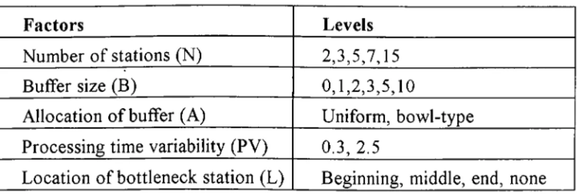
The performance of the system is measured under various conditions with the following experimental factors: 1) number of stations, 2) buffer size or buffer capacity between stations, 3) allocation of buffer capacity, 4) processing time variability, and 5) location of bottleneck station. These factors and their levels are also summarized in Table 2.1.

Table 2.1 Experimental factors and their levels

Factors Levels

Number of stations (N) 2,3,5,7,15 Buffer size (B) 0,1,2,3,5,10

Allocation of buffer (A) Uniform, bowl-type Processing time variability (PV) 0.3, 2.5

Location of bottleneck station (L) Beginning, middle, end, none

The previous studies indicate that throughput is not affected very much when the number of stations is greater than six (Conway, et al. (1988)). In our experiments, we include 15 stations to see if this upper limit is still valid· for the standard deviation of interdeparture times. For the same reasons, we use ten as a very high level for buffer capacity.

As stated in the literature, allocation of buffers is a critical factor on the system performance. We consider two types of buffer allocation; 1) uniform, 2)

(25)

CHAPTER 2. SERIAL PRODUCTION LINES 11

non-uniform (or bowl-type). In the uniform case, all buffers between stations have the same capacity. In the latter case, however, the center locations are favored with a symmetrical bowl-type allocation. To achieve bowl-type allocation, the buffer capacities adjacent to the outer stations are symmetrically transferred to the locations adjacent to the inner stations. For example, in a 5-station line with 2 buffer capacities between stations, the bowl-type allocation results in 1, 3, 3, and

1 buffer capacities in the 1st, 2nd, 3rd, and 4th locations, respectively.

Processing time (or repetitive task time) variability is also one of the most frequently studied factors in the literature. But, there is no unified agreement for coefficient of variation (CV) of processing time distribution. In the study conducted by Knott and Sury (1987) on 26 light assembly tasks, the range for CV is found to be between 0.22 and 0.57. The previous studies also indicate that repetitive task time distributions encountered in industrial applications have positive skewness, ranging from 0.3 to 3.9. In our model, we generate processing times from a lognormal distribution with a mean of 1 unit time and a coefficient of variation of 0.3. These parameters result in 0.9727 of skewness and 1.7008 of kurtosis, respectively. As seen in Table 1, we also use a very high value for the PV factor (i.e., 2.5) in order to easily see the effects of the bowl phenomenon as suggested by Hillier and So (1991).

Finally, we consider bottleneck stations and the effect of their locations on the system performance. Four levels are identified: /) bottleneck at the beginning of the line (i.e., L=l), //) bottleneck in the middle (i.e., L=2), Hi) bottleneck at the end (i.e., L=3), and /V) balanced line or no bottleneck case (L=0). A bottleneck station is created by increasing the mean processing time of that station. In our experiments, the mean processing time of the bottleneck station is set to 1.5 times that of regular stations while keeping CV constant (i.e., at 0.3).

2.4 Computational Results

In this section, we discuss the effects of the experimental factors on system performance measures and present our observations. We also attempt to draw some managerial implications from these observations.

(26)

2.4.1 Results on the Interdeparture Time Variability

We first examine the effect of the factors on the interdeparture time variability (IDTV) and confirmed the few findings reported earlier in the literature. Moreover, we analyze and elucidate several other issues related to the effect of various factors on IDTV.

1. Our first finding is on the applicability of the famous "reversibility property" in considering IDTV as a performance measure. Muth (1979) has proved that T remains invariant if the items pass through the stations in the reverse order. This result called "the reversibility property" enables to reduce the search space significantly. However, our results on the interdeparture time variability indicate that the reversibility property does not hold for IDTV (see Figure 2.2 and Figure 2.3 for a comparison). This has been also observed by Hendricks and McClain (1993). This means that the order of the stations in which items are processed is an important factor for IDTV.

Figure 2.2 Effects of Buffer Size (B) and Location of Bottleneck (L) on Throughput

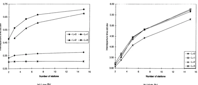
2. We also observe that the interdeparture time variability increases as the number of stations (N) increases at a decreasing rate (Figure 2.3). This is simply due to the fact that more opportunities exist for the blockage and starvation events that result in higher IDTV. This observation was previously made by Martin and Lau (1990) and Hendricks and McClain (1993).

(27)

3. Additionally, we find out that if there is a bottleneck station in the system, shifting the bottleneck station towards the end of the line (i.e., increasing L from 1 to 2 and to 3) reduces the effect of N on IDTV (Figure 2.3). The explanation of this new and important finding is as follows. Results of our simulation experiments indicate that one can identify two types of effects of a bottleneck station on IDTV: Type-1 is the increasing effect on IDTV due to the decrease in the number of units entering the system per unit time. This is due to the fact that the interdependency of the stations increases as fewer units enter the system. Type-2 is the decreasing effect on IDTV due to the mitigation of the interference of the stations upstream and downstream of the bottleneck station (e.g., a bottleneck station in the middle of the line divides the entire line into two shorter lines). As can be seen in Figure 2.3, a bottleneck station at the beginning of the line increases IDTV for any N due to mainly the Type-1 effect when compared to the non-bottleneck case. On the contrary, when the bottleneck station is at the end of the line (i.e., L=3), only Type-2 effect exists and IDTV is predominantly determined by the variability of the bottleneck station. Note that in Figure 2.3a, when L=3, IDTV is solely determined by the variability of the bottleneck station, whereas in Figure 2.3b, the effect of the other stations still exist. When the bottleneck station is between the first and the last locations (i.e., in the middle), both Type-1 and Type-2 simultaneously determine the net effect on IDTV. Hence, one should expect that the plot of the middle case to lie between the plots of bottleneck-at-the-beginning and bottleneck-at-the-end cases.

The implication of the above finding is as follows: if the existence of a bottleneck station is inevitable, then one should attempt to shift the location of the bottleneck station towards the end of the line. This can be accomplished by employing the relatively slower workers and/or assigning slower machines to the stations close to the end of the line. Note that if we consider throughput as the only performance measure, then the bowl phenomenon recommends the slower stations being located at both ends of the line (Hillier, et al. 1993). However, our finding on IDTV suggests placing the bottleneck station only at the end of the line.

(28)

(a) Low PV (b) High PV

Figure 2.3 Effects of Number of Stations (N) and Location of Bottleneck (L) on Interdeparture Time Variability

4. Another finding is about the effect of buffer size (B) on the interdeparture time variability; we observe that IDTV improves as B increases. This has also been reported by Martin and Lau (1990) and Hendricks and McClain (1993). However, we further note that the improving effect of B on IDTV is magnified as N and the processing time variability (PV) increase (Figure 2.4). This is because the effect of assigning buffer capacity is greater in longer lines in which the frequency of coupling events is relatively higher. With the same reasoning, the extra buffer capacity yields a large reduction in IDTV in the high PV case as compared to the low PV case. In addition, the effect of B on IDTV is drastically reduced when there is a bottleneck station in the system. For example, as depicted in Figure 2.5a (low PV case), the effect of B on IDTV is almost negligible for B>1. This follows from the fact that the extra buffer capacity in the system cannot effectively utilized due to the bottleneck station. The extra buffer capacity assigned to the locations upstream of the bottleneck station stay full whereas the extra capacity in the locations downstream of the bottleneck station stay idle. In the high PV case, where we have more coupling between stations, the effect of B still exists and improves IDTV (Figure 2.5b). The interaction between B and L is similar to the one observed between N and L; bottleneck-at-the-end case improves IDTV for any B when compared to the nonbottleneck case (Figure 2.5).

We can summarize the above findings as follows: First, assigning extra buffer capacity improves IDTV, but the improvement is relatively more significant in

(29)

CHAPTER 2. SEIUAL PRODUCTION LINES 15

systems with a higher frequency of coupling events (e.g., longer lines, higher PV). Thus, the cost of assigning extra buffer capacity should be carefully compared with the benefit gained by the reduction in IDTV. Since the amount of reduction in IDTV can be very small (sometimes negligible) in short lines and/or low PV cases (see Figure 2.4a). Second, existence of a bottleneck station in the system reduces the positive effect of B on IDTV. Again, we find that the best location for the bottleneck station for any B is the last location in the line.

(ajLow FV (b )H cn F V

Figure 2.4 Effects of Buffer Size (B) and Number of Stations (N) on Interdeparture Time Variability

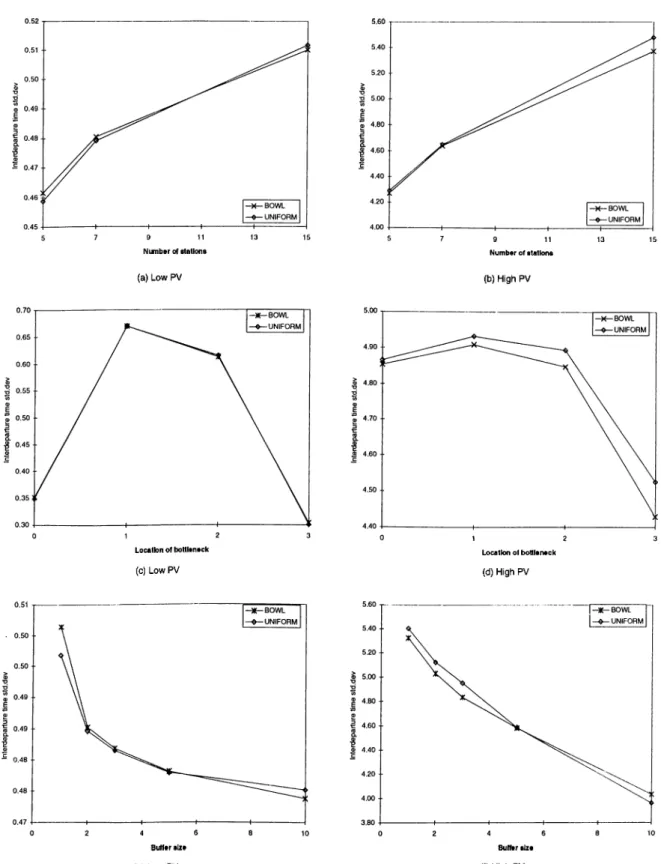
5. With respect to the allocation of buffer capacity (A), we make the following observations: First, as seen in Table 2.2, bowl type allocation has an improvement on IDTV only in the high PV case (t-test results showed that difference between the bowl and uniform allocations are significant in the high PV case). Because the high PV causes more coupling between stations and the coupling of the middle stations becomes more critical. The reason for not observing an improvement in the low PV case can be attributed to our process of designing bowl allocation. In the literature, bowl phenomenon is generally created by smoothly adjusting the mean processing times of the stations. This usually results in very smooth bowl allocation. For example, in a study conducted by Pike and Martin (1994) to determine the optimal bowl configuration on lines up to 30 stations, it is found that the maximum and the minimum processing times are 1.076 and 0.981, respectively. On the contrary, in our case, the bowl type allocation is achieved by adjusting the buffer

(30)

capacities in discrete units (similar to Hillier and So, 1991). This generally results in a non-smooth (deep) bowl allocation, and consequently does not lead to an improvement on IDTV.

6. Furthermore, as illustrated in Figure 2.6, bowl buffer allocation starts to reduce IDTV significantly in the high PV case when N and L increase and B decreases (these results are also verified by t-tests). The above findings suggest that bowl type buffer capacity allocation plays an important role in reducing the interdeparture time variability only when the frequency of coupling events is relatively higher (i.e., higher processing time variability, longer lines, and smaller buffer capacities). Note also that the effect of the bowl allocation is considerably high when the location of the bottleneck is shifted towards the end of the line.

(a)LowfV (b)HighPV

Figure 2.5 Effects of Buffer Size (B) and Location of Bottleneck (L) on Interdeparture Time Variability

Table 2.2 Effects of Buffer Allocation on Interdeparture Time Variability

IDTV(Bowl) IDTV(Uniform)

Low PV 0.4841 0.4832

(31)

CHAPTER 2. SERIAL PRODUCTION LINES 17 (a) Low PV (c) Low PV (e) Low PV Number of stations (b) High PV (d) High PV (I) High PV

Figure 2.6 Effects of Number of Stations (N), Location of Bottleneck (L), Buffer Size (B), and Buffer Allocation (A) on Interdeparture Time Variability

(32)

(c) Low PV (d) High PV

Figure 2.7 Effects of Number of Stations (N), Buffer Size (B), and Bowl-Phenomenon Created by Adjusting the Mean Processing Times on Interdeparture Time Variability

7. To obtain further insight of the behavior of the system, we conduct additional experiments and examined the effects of the traditional bowl-phenomenon as suggested in the literature (Hillier and Boling (1966)). In the new experiments, we vary N (5, 7, and 15) and B (0, 1, and 2), and create the bowl-phenomenon by adjusting the mean of processing times as recommended by Pike and Martin (1994). As depicted in Figure 2.7, the results show that the traditional bowl improves IDTV and this effect is magnified for large N and small B in the low PV case. We also note that the traditional bowl improves T but increases Q

(33)

(even though this increase was not significant at a = 0.05). Thus, we can conclude that the bowl-phenomenon (both the traditional approach and the one created by buffer capacities) has a positive effect on IDTV.

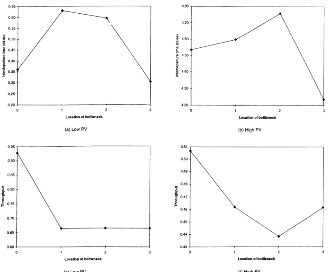
8. As discussed above, we observe that high PV causes IDTV to deteriorate in all its two-way interactions with the other factors (Figure 2.8). We also note that the inverted bowl obtained by having the bottleneck station in the middle of the line deteriorates IDTV drastically in the high PV case (Figure 2.8a and 2.8b). The same behavior is also valid for throughput (Figure 2.8c and 2.8d). In other words, the inverted bowl decreases throughput only in the high PV case.

1 2

Location of bottleneck

(c) Low PV (d) High PV

Figure 2.8 Effects of Location of Bottleneck (L) on Interdeparture Time Variability and Throughput

(34)

2.4.2 Results on the Average and Variance of WIP

Inventory

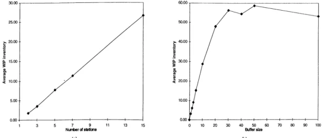
Average WIP inventory (Q) increases as N increases. As depicted in Figure 2.9a, this increase is almost linear especially for large N. The explanation of this observation can be directly made from Little's formula (Q = T * Lead time); increasing N leads to a linear increase in lead time while the decrease in T becomes insignificant after a certain value of N. Hence, the increase in Q as N increases stays linear.

The above finding on the average WIP inventory is an important one. Because the effect of N on Q does not terminate as N increases. Whereas as noted before, the effect of N on both IDTV and T decreases (it becomes almost insignificant beyond a certain value of N). Thus, one should consider the level of Q as the major controlling factor when determining the number of stations to be used in the system.

(a) (b)

Figure 2.9 Effects of Number of Stations (N) and Buffer Size (B) on Average WIP Inventory

In contrast to the throughput measure, the relationship between L and Q are strong. Q increases as the bottleneck station shifts towards the end of the line, since the buffer capacities upstream of the bottleneck station stay full. The implication of this finding is also important, because it conflicts with the earlier suggestion that shifting the location of the bottleneck station towards the end of

(35)

the line is desirable for IDTV. Hence, the decision to locate the bottleneck station in the line should be made in practice with respect to the relative importance of IDTV and Q measures.

Our results also indicate that buffer allocation has a significant impact on the average WIP. As can be intuitively expected, bowl-type allocation resulted in higher average WIP inventory compared to the uniform-type allocation.

Our last finding on the average WIP inventory is that increasing B has a negative effect on Q up to a certain level , because the excessive amount of buffer capacity between the stations stay unutilized (Figure 2.9b). Recall that increasing B improves IDTV and T at a decreasing rate (see Figure 2.6 and Figure 2.10). We also note that the effect of increasing B on Q exists for a much larger range when compared with the effect on IDTV and T. Combining the above findings, we can conclude that the benefits gained from assigning buffer capacity becomes minimal after a certain value of B. Hence, the decision to set the amount of buffer capacity should be made cautiously, since the associated cost figures can be of a significant size.

(a) (b)

Figure 2.10 Effects of Buffer Size (B), Processing Time Variability (PV) and Number of Stations (N) on Throughput

(36)

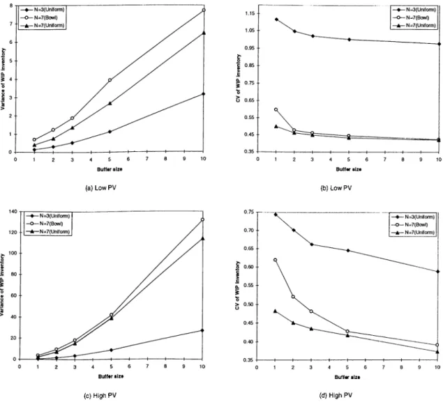
Finally, we examine the effects of the design factors (N, L, PV, and B) on the variability of WIP inventory. Both the variance and CV of WIP inventory are measured in the experiments. The variance (or CV) is important to construct a confidence interval on the average WIP. Because, this additional information can be utilized by designers to set the upper limits on buffer capacities (i.e., buffer capacities can be set to lower values if the design results in a smaller variance).

As depicted in Figure 2.11, the variance of WIP increases as the buffer size increases. This is especially observed in the high PV case with longer line lengths and bowl-type buffer allocation. This counter-intuitive result (i.e., observing a deterioration in the system performance even though the available resource is increased) is due to the fact that WIP can fluctuate in a wider range of buffer capacity. On the contrary, however, we also note that CV of WIP decreases as B increases due to the much larger increase in the average WIP. The above findings support our previous conclusions and suggest that designers should not increase B beyond a certain limit.

We also study the effect of L on the variance (and CV) of WIP. Since, according to our previous results, PV plays an important role in describing the effect of the bottleneck station, we analyze the high and low PV cases separately.

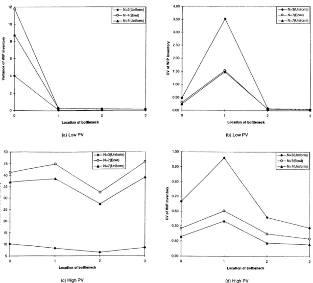
i) As illustrated in Figure 2.12a, in the low PV case, the existence of a bottleneck station improves the variance of WIP. This is due to the fact that buffers upstream of the bottleneck station stay full whereas the buffers downstream of the bottleneck station stay empty. This leads to a lower variance compared to the nonbottleneck case. Examining the effect of L on the CV of WIP (Figure 2.12b) reveals that as the level of L increases, the CV decreases except for L=l. In this exception case, the average of WIP is considerably smaller than the level in the nonbottleneck case that results in the higher CV For the other locations of the bottleneck station, the average WIP increases with smaller variance; hence, the net effect reduces the value ofCV.

ii) Similar to the low PV case, the same pattern of CV has been observed in the high PV case (Figure 2.12d). However, we note an unexpected behavior of the variance of WIP for the L=2 level in the high PV case. As illustrated in Figure 2.12c, the variance of WIP decreases only when the bottleneck station

(37)

is at the middle of the line. This situation arises because the L=2 level divides the entire line into two shorter lines which leads to smaller variances (recall that increasing N has an increasing effect on the variance of WIP in the high PV case). Note also that the negative effect of bowl allocation is observed only in the high PV case.

(a) Low PV (b) Low PV

(c) High PV (d) High PV

Figure 2.11 Effects of Location of Bottleneck (L), Processing Time Variability (PV), and Number of Stations (N) on Variance and CV of WIP Inventory

(38)

(a) Low PV

(c) High PV

(b) Low PV

Location o f bottleneck

(d) High PV

Figure 2.12 Effects of Location of Bottleneck (L), Processing Time Variability (PV), and Number of Stations (N) on Variance and CV of WIP Inventory

2.5 Discussion

In the first part of the thesis, we studied the unpaced and asynchronous serial production lines with reliable machines. Specifically, we analyzed the problem for the interdeparture time variability and average WIP inventory measures. Based on our simulation experiments and statistical analysis of the results, we have obtained several new findings about the effect of various system design parameters on the interdeparture time variability and average WIP inventory. We have also

(39)

confirmed some of the results reported earlier in the literature. These new findings and the related managerial implications are summarized as follows:

1. Similar to the throughput measure, increasing the line length deteriorates the interdeparture time variability at a decreasing rate. This effect is more noticeable in systems with higher processing time variability. When there is a bottleneck station in the system, shifting it towards the end of the line reduces the effect of line length on the interdeparture time variability.

2. The location of the bottleneck station plays an important role for the interdeparture time variability. Results of the experiments indicated that the interdeparture time variance changes from the highest value (when the bottleneck is the first station in the line) to the lowest value (when the bottleneck is the last station in the line). Moreover, the interdeparture time variability associated with the non-bottleneck case is found to be between these two extreme values. In contrast to the throughput case, this new finding suggests that a carefully selected location for the bottleneck station can indeed improve the interdeparture time variability when compared to the non bottleneck case. In our study, we also found that the location of the bottleneck station affects throughput in the high processing time variability case. Hence, by considering both throughput and interdeparture time variability, we suggest to locate the bottleneck station towards the end of the line.

3. Even though shifting the location of the bottleneck station towards the end of the line minimizes the interdeparture time variability (recall that it has no effect on throughput for the low PV case), it is not desirable for the average WIP inventory measure since more items tend to accumulate in the buffers upstream of the bottleneck station. Thus, one should consider a tradeoff between the interdeparture time variability and WIP inventory in locating the bottleneck station. Our results also indicated that the bottleneck station should be located in the middle of the line when considering the variance of WIP.

4. A similar tradeoff exists between the performance measures (S, T, Q, and variability of WIP) when the number of stations is considered. Unlike the interdeparture time variability and throughput, the effect of the number of stations on the average and variance of WIP inventory does not terminate as the number of stations increases. Also, unlike the other performance measures.

(40)

CV of WIP decreases as the line length increases, Thus, a system designer should find a compromise between the above performance measures in setting the optimal line length.

5. We found that assigning extra buffer capacity improves the interdeparture time variability. This effect is more prominent in systems with higher processing time variability and number of stations. However, the existence of a bottleneck station reduces this improving effect drastically. In contrast to throughput and interdeparture time variability, buffer capacity has a negative effect on the average and variance of WIP, but not on the CV of WIP inventory. Also, the effect of buffer capacity on the average WIP inventory exists for a much larger range when compared to the effect on throughput and interdeparture time variability. Since the effect of buffer capacity on various performance measures are different and there is a cost associated with assigning extra buffer capacity, system designers should determine the level of buffer capacity cautiously.

6. Similar to the throughput measure, bowl-phenomenon has a positive effect on the interdeparture time variability. This effect is noticeable in both the traditional approach and the one created by buffer capacities in this study. Unlike the other performance measures, bowl phenomenon deteriorates both the variance and CV of WIP. Hence, this downside effect should be measured against the benefits of the bowl phenomenon.

(41)

C hapter 3

ASSEM BLY SYSTEM S

3.1 Introduction

In this part of the study, we consider the problem of designing an assembly system in which parts produced at two or more component stations are fed into an assembly station. In general, assembly systems are comprised of three main building blocks: serial, merging and splitting (competing) configurations. Most of the existing work to date is conducted on serial systems although merging and splitting are also common configurations encountered in practice. In this chapter, however, we concentrate on the merging configuration and examine its various characteristics.

A key criterion in the design and operation of assembly systems has been throughput which is measured as the number of units produced per unit time. Output variability (or interdeparture time variability) is also important especially in today’s highly dynamic and stochastic environments, since a highly variable input or output process makes planning difficult and causes the performance to deteriorate significantly. Hence, practitioners designing such assembly systems should consider interdeparture time variability in addition to throughput. In this study, we consider both throughput and interdeparture time variability and analyze the effects of design factors such as parallelism (given by the number of component stations), processing time distributions, work and variability transfers from the assembly station to component stations, buffers and buffer allocation schemes. We also study the so called “intrinsic behavior of the optimal throughput

(42)

for some processing time distributions” (Baker, Powell and Руке (1993); Rekhi, Chand and Moskowitz (1995)) and uncover the underlying details.

The rest of this chapter is organized as follows. In Section 3.2, we summarize the relevant literature on assembly system design. In Section 3.3, we present the proposed approach, system considerations, and experimental design. The results of simulation experiments are presented in Section 3.4. In Section 3.5, we explain the intrinsic behavior. Later, we extend our analysis to the buffered case in Section 3.6. This chapter ends with concluding remarks in Section 3.7.

3.2 Literature Survey

There are only a few and limited studies on this problem. They are briefly summarized in a chronological order below.

Baker, Powell and Руке (1990) examine the design of balanced assembly systems with variable processing times under two loading mechanisms. The term

'Ъа1апсесГ refers to identically distributed component and assembly station

processing times. For all processing time distributions, the authors observe that the push mode results in higher throughput than the pull mode since an assembly system utilizes the virtual buffer existent in the assembly station under the push mode. The authors also analyze the effects of buffers on throughput of assembly systems composed of two feeder lines where each feeder is a serial line. They note that the results from the serial line research generally apply to such systems. In addition, the authors observe that a small buffer is sufficient to recover the significant portion of the lost capacity and that equal buffer allocation is desirable for these systems.

Later, Baker, Powell and Руке (1993) examine the problem of allocating a fixed amount of work to stations in an assembly system operating under the push mode. For systems up to four component stations with exponentially distributed processing times, Markov analysis is used, whereas simulation is used for other distributions and larger systems. Their basic finding is that throughput can be improved by transferring work from the assembly station to component stations. The authors also study two specific unbuffered assembly systems for exponential and uniform processing time distributions. The first one is a system with two

(43)

CHAPTER 3. ASSEMBLY SYSTEMS 29

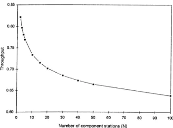
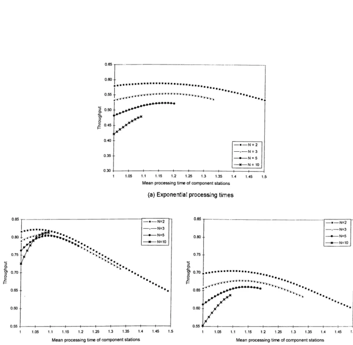
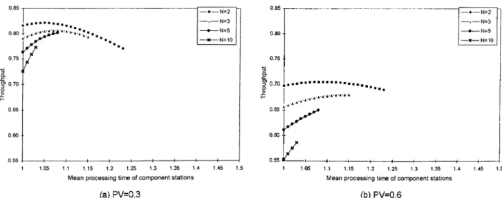
feeder lines where each feeder line is composed of two stations. Their results indicate that throughput is maximized by allocating more work to the initial stations and less work to the final stations of the feeder lines and assembly station. The second system involves two or more component stations in parallel. The results show that optimal throughput is a decreasing function of the number of the component stations. However, this phenomenon is not observed for the uniform distribution; instead, optimal throughput displays a small peak in a specific range. We call this anomaly “hump behavior” in this study. In a later study (but published earlier). Baker (1992) presents a brief survey on serial lines and assembly systems. He notes that the above unexpected behavior might be due to the lower coefficient of variation (cv) of the uniform distribution.

Bhatnagar and Chandra (1994) examine the impact of different types of variability (processing time, unreliable stations and imperfect yield) on the throughput of assembly and competing systems. They find out that the cv of processing times is a critical criterion for studying the impact of processing time variability in assembly systems.

Later, Rekhi, Chand and Moskowitz (1995) study assembly systems with up to 100 component stations for exponential, uniform, gamma and normal processing time distributions with different cv’s. The results indicate that as the number of component stations increases, optimal throughput steadily deteriorates for the distributions that have small tails such as exponential and high-cv gamma. However, they observe the hump behavior for distributions with long tails such as uniform, normal or low-cv gamma. The authors explain this behavior with the long tails of the above distributions. In this study, we further examine this behavior and uncover the underlying details.

In another study. Baker and Powell (1995) present a predictive model for the throughput o f an assembly system with two component stations. They develop a distribution-free method to evaluate alternative system designs and claim that the algorithm performs well in terms of the accuracy of the predictions.

Simon and Hopp (1995) analyze an assembly system with two component stations. There are finite buffers between each component and the assembly station. The authors develop a stochastic model to estimate the steady-state average throughput and inventory level performances.