An Assessment on the Importance of the Credit Channel in Eastern Block Countries

(1)

An Assessment on the Importance of the Credit Channel in

Eastern Block Countries

Prof. Dr. Ahmet Ay (Selçuk University, Turkey)

Assoc. Prof. Dr. Zeynep Karaçor (Selçuk University, Turkey)

Ph.D. Candidate Nazan Şahbaz (Karamanoğlu Mehmetbey University, Turkey)

Abstract

Monetary policy carried out by monetary authority affects by means of monetary transmission channels consisting of traditional interest channel, asset prices channel, exchange rate channel, credit channel, and expectation channel. Credit channel forming the main subject of this study is divided into two subclass such as channel of bank credit and channel of balance sheet. The objective of this study is to study the effects of bank credits channel in Bulgaria, China, Hungary, and Poland, countries of East Bloc in 1994-2010. In analysis, as indicator of momentary policy, interest rate is taken and the effect of variations in real interest rate on the economy. In the context of effects on economy, the rate of unemployment, inflation and total credit volume are taken into consideration. In testing the stability of the data used in analyses, ADF Unit Root test was utilized. In determining the direction of relationship between variables, in the scope of Granger Causality Test and VAR model, impulse-response functions were used.

1 Introduction

In monetary transmission mechanism, credit channel plays role through bank credits channel, and balance sheet channel. The most important function of bank credit channel, bringing those having fund surplus and those needing fund into together, is to create extra power to purchase in favor of those needing fund.

That credit channels are important transmission mechanism has three important reasons. Firstly, the shortcomings in credit channels is important in the run of credit channels and this situation affects the decisions of the expenditure and unemployment of the firms. Secondly, small firms, whose risk to face credit constraint is higher than the large firms, are more negatively affected from the tight monetary policy compared to large firms. Lastly, the view that “the shortcomings in credit markets revealed the problem of deficient informing” that forms the base of credit channel analysis, in terms of explaining a number of phenomena that are important, presents as a powerful instrument (Mishkin, 2000:289).

Mishkin (1995) divided the transmission channel into interest channel, exchange rate channel, asset prices channel, and credit channel. In some studies, a division is made as monetary view (traditional interest channel) and credit view (credit channel). (Bernanke, 1988:3-11, Bernanke, 1993:55-57; Cecchetti, 1999:13). In credit view, banks play active role. Mechanism runs in the way that following contractionary monetary policy, contraction of bank the credit volume, and depending on the contraction in credit volume, bank dependent firms are obliged to reduce the investments.

In this study, credit channel of monetary transmission of East Block Countries are examined. In this frame, monetary transmission mechanism was examined in theoretical frame and empirical studies conducted on credit channels were given place. In the last section of the study, in order to examine the credit channel of the countries such as Bulgaria, China, Hungary, and Poland, the analysis of impulse-response functions was given. In analysis, as the indicator of monetary policy , real interest rate was taken and it was suggested how the variations in real interest rate affected total credit volume, unemployment rate, and inflation. For this purpose, first of all, unit root analysis was carried out for the variables and then for the variables brought into stable in the same degree, co-integration test, and Granger causality test was conducted. Finally, the impulse-response functions of variables were taken place.

2 Literature

The findings of studies analyzing the run of bank credit channel are different from each other. In academic studies conducted in his area, predominantly as an indicator of monetary policy, real interest rates were used and in large part of the studies, the effects of monetary policy that externally changes on macroeconomics were examined on the basis of VAR.

Bernanke and Blinder (1992), in order to examine the importance of bank credit channel, in this study carried out by using VAR model and covering the period of 1959 - 1978, it was concluded that federal interest rate was a good indicator of monetary policy and in the face of the variations in this rate, the reaction of bank deposit, bank securities stock, bank credits, unemployment rate, and prices was examined. As a result of contractionary monetary policy, it was seen that banks reduced the investment of securities more rapidly than credits. This development was explained by the nature of credit contracts. According to this, that credit contracts cover a certain term, prevented the credit from rapidly contracting. However, in two periods, contraction in bank credit

(2)

exceeded the contraction in security stock. In addition, the movements in bank credit and real activity were observed to be simultaneous. These findings were interpreted that credit channel run; however, at the beginning, due to the fact the contraction in securities was more than that in the credits, and that the operability was partial.

Kashyap and Stein (1994), in their studies, emphasizing the scale of banks giving credit, examined the effect of tight monetary policies on the credit supply. In their studies, they determined that tight monetary policies did not create any variation in the credit supply opened by small scaled bank, however, in credit supply opened by large scaled banks, that there was a decrease. According to Kashyap and Stein, this difference between small banks and large banks, is resulted from that small banks, in the conditions of tight monetary policy, cannot met the decrease occurring in their deposits, like large firms, by alternative financial resource.

Gunduz (2001), examined the role of bank credit channel, using VAR analysis. In this study, covering the period of 1986 -1998, following monetary policy, one regarded at what measure and in what direction the variation occurred. Following the contractionary monetary policy, bank credits and securities were observed to decrease very rapidly. That the decrease in securities was in serious dimensions was interpreted in the way that the role of credit channel in monetary transfer mechanism was limited.

Schmitz (2004) tested the properties of bank credit channel in transition countries, using the data from the balance sheets of 261 bank in Czech Republic, Estonia, Hungary, Leetonia, Lithuania, Poland, Slovakia, and Slovenia. In the countries of European union, the increase of 1% point in interest rates reduced the credit growth by 1.8%, and 2% in the next year. Schmitz confirmed the view that only bank size affected the monetary transmission through credit channel and that bank capitulation did not have any role.

Ferreira (2007), especially Portugal, in the countries that are member to European Monetary Union, tested the run of credit channel, using the data belonging to the period of 1990 -2002 by means of panel data method. For posing the importance of bank performance in the run of credit channel, the study he carried out, Ferreira reached the conclusion that credit channel was a basic channel of monetary policy, however, that in the run of this channel, bank performances and strategies were effective.

3

Theoretical Approaches to Transmission Mechanism

The concept of monetary transmission mechanism are used to express the effects of money on total output (GDP) and total expenditures (nominal GDP) and the transmission channels running in the emergence process of these effects (Mishkin, 1992: 657-658; Petursson, 2001: 62-63).

3.1 Keynesian Transmission Mechanism

According to the theory of Keynesian liquidity preference, except of liquidity trap, interest rate shows sensitivity to the variation in monetary supply. This situation, effecting the investments will cause the income level to rise via multiplier. According to the portfolio approach, to the relative returns of alternative investment instruments are regarded as only one factor affecting the choice of portfolio (Altunöz, 2010:62).

In general theory, the process of transmission mechanism runs in such a way. First, the increase in monetary stock affects the interest rate; the decrease in interest rate affect investment, investment the demand, demand the expenditures, and all process the total income (Laidler, 1982: 112).

3.2 Monetarist Transmission Mechanism

It can be said that monetarist transmission mechanism is not something than the known quantity theory. According to mechanism, monetary stock is external and only depends on the behavior of monetary authority. Money directly affects the nominal expenditures. In the short period, if economy is a near place to the level of full employment, money only affects the general level of prices, does not affect employment. If economy is below the income level of full employment, the increase in monetary stıck affects the real income; in long term, the increase in monetary stock only affects the general level of prices (Friedman, 1987: 3-5 ).

4 Credit Channel

There are asymmetric information problem on the basis of credit channel. Asymmetric information states the case, where those supplying financial resources do not have sufficient information about those demanding it and the possibility of firms to utilize every kind of financing form, due to asymmetric information, are removed (Cengiz, 2009:235). Credit channel can be divided into two separate channels as banking credit channel and broad lending channel (Egert ve Macdonald, 2006: 16). In credit channel, monetary policy affects the economy through two channels completing each other as bank credit channel and balance sheet channel. Bank credit channel emphasizes the role of banks in financial structure. Unlike the traditional interest channel, in bank credit channel, three actives different from each other, namely money, security, and bank credit, are taken into consideration and bank credit and security are assumed not to fully substitute each other. For example, as a result of contractionary monetary policy, in case that banks compensate the decrease occurring in their reserves by contracting credit supply instead of selling security, bank credit channel plays important role in monetary transmission mechanism. (Bernanke and Blinder, 1988: 435)

(3)

In credit view, instead of classifying all of financial actives under a single category, the requirement of classification as the funds obtained from bank – non-bank resources, and more generally, in the form internal-external financing, is emphasized. In this way, making an emphasis the heterogeneity among borrowers, it is expressed that the borrowers are exposed to the variations in credit conditions more compared to the others (Walsh, 1998:285).

5 Bank Credit Channel

Bank credits channel, influencing the bank credit volume, expresses the process to influence the total demand, in turn, product of monetary policy implementation (Erdoğan-Beşballı,2009: 29 ), As a result of contractionary monetary policy, since bank reserves and deposits will rise up, the amount of credit the banks can give will increase. The increase in the amount of credit leads especially investment expenditures of small and medium sized enterprises to rise. Credit channel mostly affects the investment expenditures of small and medium sized enterprises, because small firms are excessively dependent on the bank credits to meet their financing needs. The large firms have the power to be able to meet their fund needs from the stock and bond markets . Hence, through credit channel, it can be said that the shocks occurring in monetary policy can affect the small firm much more (Ornek, 2009: 106).

For the credit channel to run independently , it is necessary to provide three conditions: (i) credits and bonds that are supplied to the public must not be full substitution; (ii) Central bank (CB, modifying the amount of reserve, must influence the supply of credit; (iii) price regulation must not be full sot that it can prevent monetary policy from being neutral (Telatar, 2002: 91).

In the transmission process of monetary policy, one of the most important conditions providing the banks to undertake an active role is that economic units that are dependent on the bank about external financing credit take place. In this way, since these borrowers will be directly affected from the variations of credit supply of banks, with the other credit channel, a transmission process will have been realized. However, under these conditions, with the effect of monetary policy implemented, The effects of variations occurring in credit supply on the real economy will emerge (Meltzer,1995: 49-52 )

The run of credit channel is affected from the various factors such as the economic structure of country, financial system and composition of balance sheets of actors, and maturity structure of financial actives. In addition, it is known that the chronic inflation process affected the monetary transmission process, and especially via interest rate and asset prices, reduced it. Besides these, the increasing interest rates and realizing rapid exchange rate increases caused the equities of banks to significantly decrease and that banks prefer to remain liquid (Inan, 2001:18).

6 Methodology and Model

Ozgen and Guloglu (2004), VAR models are used in the relationships between macroeconomic variables and in studying the effect of random shocks on the system of variable

VAR analysis can be simply shown as follows. VAR model can be put in order in two ways as structural and standard. Via matrix notation, structural VAR model can be written as follows:

BX t = r0 + r1 X t −1 + r2 X t −2 + …… rp X t – p+ ut (1)

In Equation 1 , X t is a vector included in the model and that includes each of 10 variables. r0 is constant terms vector (n ∗1 ). . ri , i=1,…, p (𝑛 ∗ 𝑛) are the matrices of coefficients. ut states the shocks to the variable in the model. B, denotes the synonymous feedback between the elements of X t . Equation 1 supposed that X t is stable. uts denote error terms whose expected value is zero, variance constant, and covariance zero.

The above model, multiplying by

B −1 both sides of the equation, can be turned into the reduced VAR Model.

X t = A0 + A1 X t −1 + A2 X t −2 +…….+ Ap X t − p et (2)

Here, 𝐴0= 𝛽 −1_𝑟

0, 𝐴1= 𝛽−1𝑟1, … … . . , 𝐴𝑝= 𝛽−1𝑟𝑝

In Equation 2, A0, is a vector of constant terms (n ∗ 1). A1 is matrices of coefficients (𝑛 ∗ 𝑛) and 𝑒𝑡 is vector of

error terms (n ∗ 1) . Equation 2 is a reduced form of Equation 1. 𝑒_𝑡 should be considered to be the component of error terns in 𝑢_𝑡. Since the elements of 𝑢_𝑡 are white noisy, the elements of 𝑒_𝑡 have average zero and fixed variance and there is also no correlation between them. But between the equations of error terns in 𝑒_𝑡, variance covariance matrix has a correlation stated by ∑. The reason for this is that the variables have current effects on each other.

In Equation 2, matrix 𝐴₀ denotes constant term and each includes n2 coefficients of matrix 𝐴_𝑖. In view of this, it is necessary to predict the terms 𝑛 + 𝑝𝑛2. Right side of Equation 2 contains only already determined variables. It is supposed that error terms have constant variance and that there is no correlation between them. In view of

(4)

this, each equation is estimated by using the method of Lest Squares (LS). However, in this case, it can faced to the determination problem. The reasons for this is that the numbers of parameters predicted by using standard VAR model is never enough to obtain the parameters in structural VAR.

In addition, VAR can be in the form of vector moving average (VMA). Indication of VMA allows for us to follow the trajectory of shocks on various variables included in VAR system in time. For example, VMA enables us to obtain the cause –effect functions. VMA indication of Equation 2 can be written as follows:

X t = µ + ∑∞𝑗=0𝛷𝑗𝑒𝑡−1 ₍₃₎

It was indicated as 𝑒_{𝑡= 𝛽}−1_𝑢 𝑡

If we substitute this relationship in Equation, the following form can be obtained:

𝑋 𝑡 = 𝜇 + ∑∞_𝑗=0𝛷𝑗𝛽−1𝑢𝑡 ₍₄₎

For being able to write Equation 5 as follows, it can be expressed as 𝛹𝑗= 𝛷_𝑗𝛽−1

𝑋 𝑡 = 𝜇 + ∑∞_𝑗=0𝛹𝑗, 𝑢𝑡 ₍₅₎

The coefficient of 𝛹_𝑗 are called impulse-response function. The coefficient of 𝛹_𝑗 can be used to introduce the effects of structural _𝑢_𝑡_{shocks on all trajectory of the variation 𝑋}_𝑡_{. In addition, from the coefficients of 𝛹}_𝑗, i total effects of each shock on the other variables can be reached or effect factors (Ozturkler, 2002).

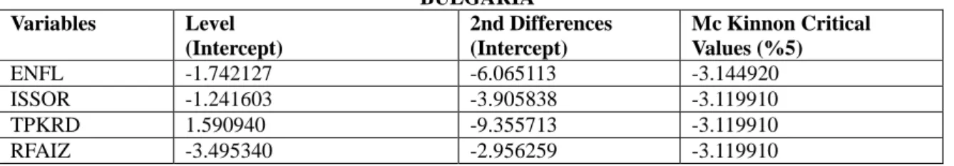
For an effective and consistent VAR analysis, all variables in the model should be stable. Stability is generally determined by Unit Roots and thus it is decided whether the variables can be formulated as level or taking their difference In this study, Augmented Dickey Fuller (ADF) test, one of the most commonly used tests, was used. Adding the fixed and trend variables to regression, the results obtained from the tests of ADF (ττ)) unit root null hypothesis are shown below. In analysis, data was obtained from the World Bank. In analysis, the variable inflation was denoted as (ENFL), unemployment rate as (ISSOR), total credit volume as (TOPKRD) and real interest rate as (RFAIZ).

Before passing to the prediction of VAR model, the suitable lagging length was determined for model. In determining optimum lagging level, it was seen that the values of LR (Likelihood Ratio), FPE (Final Prediction Error) and AIC were in the same direction and they gave minimum value for 7 lags; and the values of SC and HQ (Hannan-Quinn Information Criterion) provided minimum value for 2 lags. Upon that the other three criteria give minimum value, it was determined that optimum lagging level used in analysis was 7.

BULGARIA Variables Level (Intercept) 2nd Differences (Intercept) Mc Kinnon Critical Values (%5) ENFL -1.742127 -6.065113 -3.144920 ISSOR -1.241603 -3.905838 -3.119910 TPKRD 1.590940 -9.355713 -3.119910 RFAIZ -3.495340 -2.956259 -3.119910

Table1: Results of Unit Root Test

According to the results of test statistic taking place in Table 1, it was determined that the variable RFAIZ was stable at the level of I(1) and that the variables ENFL, ISSOR, TOPKRD became stable at the level of I(2). In order to identify that there was a long termed relationship between becoming stable at the same level, Johansen co-integration test was utilized and the results of analysis were summarized by means of Table 1.

Eigenvalue Trace Statistic Critical Value (%5) ENFL ISSOR TOPKRD 0.980242 90.08094 29.79707 0.902041 35.14224 15.49471 0.170520 2.617380 3.841466

Table 2: Results of Johansen Co-integration Tests

The values of test statistic arranged inTable 2 is the parameters of “Co-integration Likelihood Rate”. According to these results, it was determined that there was co-integration between ENFL and ISSOR. In order to determine whether or not there was a causality relationship between variables, even though co-integration was under consideration, Granger causality test was utilized and the results of analysis were arranged in Table 3.

(5)

H0 Hypothesis Observation F-Statistics Prob.

ISSOR does not Granger cause ENFL 14 0.27179 0.76805

ENF, does not Granger cause ISSOR 1.55046 0.26388

Table-3: Results of Granger Causality Test

When Table 3 was examined, it was determined that there was a double directional causality relationship between unemployment rate and inflation in the meaning of Granger.

Since interpreting coefficients obtained from VAR analysis was rather difficult, in the face of the shocks to be applied to the equation systems, “cause -effect” analysis measuring the reaction the variables will give is interpreted. By means of cause- effect analysis, in the face of the shocks orderly to be applied to any variable taking place in the model, the possibility to measure the reactions of the relevant variable and other variables is obtained. (Lütkepohl and Saikkonen, 1997:127-157).

Figure 1: Impulse-response Functions

CHINA Variables Level (Intercept) 2nd Differences (Intercept) Mc Kinnon Critical Values (%5) ENFL -3.750571 - -3.212696 ISSOR -3.891043 -8.665148 -3.119910 TPKRD -1.325125 -3.451250 -3.144920 RFAIZ -3.451250 - -3.144920

Table-4: Results of Unit Root Test

As will be seen in in the third panel of first line in Figure 1, in case that a shock of one standard deviation was applied to the real interest, in the first good period inflation, it causes an increase and loses its effect after the second period. In third panel of third order, applying shock to the real interest causes to decrease in total credits, beginning from the first period and loses its effect beginning from sixth period.

According to the results of ADF test statistics taking place in Table 4, it was determined that the variables ENFL and RFAIZ were in normal and that the variables ISSOR, TOPKRD became stable at the level of I(2). Between the variables becoming stable at the same level, in order to determine that there was a long termed relationship Johansen Co-integration test and the results of analysis were summarized in Table 5.

Eigenvalue Trace Statistic Critical Value (%5) ENFL RFAIZ 0.832400 36.02298 15.49471 0.544744 11.01655 3.841466 ISSOR TOPKRD 0.377204 9.545710 15.49471 0.188036 2.916192 3.841466

Table-5: Results of Johansen Co-integration Tests

0 20 40 60 80 100 1 2 3 4 5 6 7 8 9 10

Perc ent EN FL v ariance due to EN FL

0 20 40 60 80 100 1 2 3 4 5 6 7 8 9 10

Perc ent EN FL v ariance due to ISSOR

0 20 40 60 80 100 1 2 3 4 5 6 7 8 9 10

Perc ent ENFL v ariance due to R FAIZ

0 20 40 60 80 100 1 2 3 4 5 6 7 8 9 10

Perc ent EN FL v ariance due to TOPKR D

0 10 20 30 40 50 60 70 80 90 1 2 3 4 5 6 7 8 9 10

Percent ISSOR v ariance due to EN FL

0 10 20 30 40 50 60 70 80 90 1 2 3 4 5 6 7 8 9 10

Perc ent ISSOR v ariance due to ISSOR

0 10 20 30 40 50 60 70 80 90 1 2 3 4 5 6 7 8 9 10

Percent ISSOR v ariance due to R FAIZ

0 10 20 30 40 50 60 70 80 90 1 2 3 4 5 6 7 8 9 10

Percent ISSOR v ariance due to TOPKRD

0 10 20 30 40 50 1 2 3 4 5 6 7 8 9 10

Perc ent R FAIZ v ariance due to EN FL

0 10 20 30 40 50 1 2 3 4 5 6 7 8 9 10

Perc ent R FAIZ v arianc e due to ISSOR

0 10 20 30 40 50 1 2 3 4 5 6 7 8 9 10

Percent RFAIZ v ariance due to RFAIZ

0 10 20 30 40 50 1 2 3 4 5 6 7 8 9 10

Percent R FAIZ v ariance due to TOPKRD

0 10 20 30 40 50 60 70 1 2 3 4 5 6 7 8 9 10

Percent TOPKR D v ariance due to EN FL

0 10 20 30 40 50 60 70 1 2 3 4 5 6 7 8 9 10

Percent TOPKR D v ariance due to ISSOR

0 10 20 30 40 50 60 70 1 2 3 4 5 6 7 8 9 10

Percent TOPKRD v arianc e due to R FAIZ

0 10 20 30 40 50 60 70 1 2 3 4 5 6 7 8 9 10

Percent TOPKR D v ariance due to TOPKR D

(6)

The values of test statistics arranged in Table 5 are the parameters of “Co-integration Likelihood Rate”. According to these results, it was determined that there was a co-integration between ENFL and RFAIZ. Between the variables where there was a co-integration, in order to determine whether there was a causality or not in the meaning of Granger, Granger causality test was utilized and the results of analysis was arranged in Table 6.

RFAIZ does not Granger cause ENFL 14 0.09584 0.09584

ENFL does not Granger cause, RFAIZ 0.12416 2.65396

When Table 6 is examined, there was a double directional relationship between unemployment rate and inflation in the meaning of Granger.

Figure-2: Impulse-response Functions

As will be seen in the first panel of first line in Figure 3, in case that a shock of one standard deviation was applied to the unemployment rate, inflation causes the increase after eightieth period .

In third panel of the first, second, third, and fourth line, applying shock to the real interest caused any change in unemployment rate and real interest.

According to the results of ADF test statistics taking place in Table 7, it was determined that the variable RFAIZ was in normal level and that the variables ENFL, ISSOR and TOPKRD became stable at the level of I(2). Between the variables becoming stable at the same level, in order to determine that there was a long termed relationship Johansen Co-integration test and the results of analysis were summarized in Table 8.

HUNGARY Variables Level (Intercept) 2nd Differences (Intercept) Mc Kinnon Critical Values (%5) ENFL -1.289657 -4.417733 -3.212696 ISSOR -0.756440 -3.842263 -3.175352 TOPKRD -1.283773 -6.662001 -3.119910 RFAIZ -3.300135 - -3.081002

Eigenvalue Trace Statistic Critical Value (%5) ENFL ISSOR TOPKRD 0.944816 60.04853 29.79707 0.640565 19.48929 15.49471 0.308484 5.164175 3.841466

-400 -200 0 200 400 600 800 1 2 3 4 5 6 7 8 9 10

Response of ENFL to ENFL

-400 -200 0 200 400 600 800 1 2 3 4 5 6 7 8 9 10

Response of ENFL to ISSOR

-400 -200 0 200 400 600 800 1 2 3 4 5 6 7 8 9 10

Response of ENFL to RFAIZ

-400 -200 0 200 400 600 800 1 2 3 4 5 6 7 8 9 10

Response of ENFL to TOPKRD

-800 -600 -400 -200 0 200 400 1 2 3 4 5 6 7 8 9 10

Response of ISSOR to ENFL

-800 -600 -400 -200 0 200 400 1 2 3 4 5 6 7 8 9 10

Response of ISSOR to ISSOR

-800 -600 -400 -200 0 200 400 1 2 3 4 5 6 7 8 9 10

Response of ISSOR to RFAIZ

-800 -600 -400 -200 0 200 400 1 2 3 4 5 6 7 8 9 10

Response of ISSOR to TOPKRD

-800 -600 -400 -200 0 200 400 1 2 3 4 5 6 7 8 9 10

Response of RFAIZ to ENFL

-800 -600 -400 -200 0 200 400 1 2 3 4 5 6 7 8 9 10

Response of RFAIZ to ISSOR

-800 -600 -400 -200 0 200 400 1 2 3 4 5 6 7 8 9 10

Response of RFAIZ to RFAIZ

-800 -600 -400 -200 0 200 400 1 2 3 4 5 6 7 8 9 10

Response of RFAIZ to TOPKRD

-4000 -3000 -2000 -1000 0 1000 2000 1 2 3 4 5 6 7 8 9 10

Response of TOPKRD to ENFL

-4000 -3000 -2000 -1000 0 1000 2000 1 2 3 4 5 6 7 8 9 10

Response of TOPKRD to ISSOR

-4000 -3000 -2000 -1000 0 1000 2000 1 2 3 4 5 6 7 8 9 10

Response of TOPKRD to RFAIZ

-4000 -3000 -2000 -1000 0 1000 2000 1 2 3 4 5 6 7 8 9 10

Response of TOPKRD to TOPKRD

(7)

The values of test statistics arranged in Table 8 are the parameters of “Co-integration Likelihood Rate”. According to these results, it was determined that there was a co-integration between ENFL, ISSOR and TOPKRD. Between the variables where there was a co-integration , in order to determine whether there was a causality or not in the meaning of Granger, Granger causality test was utilized and the results of analysis was arranged in Table 9.

ISSOR does not Granger cause ENFL 14 3.74227 0.06565

ENFL does not Granger cause ISSOR 0.57905 0.58001

TOPKRD does not Granger cause ENFL 14 2.30002 0.15601

ENFL does not Granger cause TOPKRD 2.52238 0.13498

TOPKRD does not Granger cause ISSOR 14 9.10039 0.00689

ISSOR does not Granger cause TOPKRD 3.95529 0.05853

When Table 9 is examined, it was determined that there was only a double directional relationship between inflation total credit volume in the meaning of Granger.

In the fourth panel of first line in Figure 3, in case that a shock of one standard deviation was applied to the real interest rate, an increase occurred until the second period and then a decrease emerged until third period and after that, any variations did not occur.

POLAND Variables Level (Intercept) 2nd Differences (Intercept) Mc Kinnon Critical Values (%5) ENFL -4.097911 - -3.081002 ISSOR -4.212358 - -3.119910 TPKRD -2.115727 -7.149608 -3.119910 RFAIZ -1.538446 - -3.098896

According to the results of ADF test statistics taking place in Table 10, it was determined that the variable ENFL and ISSOR were in normal level and that the variable TOPKRD became stable at the level of I(2). Between the variables becoming stable at the same level, in order to determine that there was a long termed relationship Johansen Co-integration test and the results of analysis were summarized in Table 11.

0 20 40 60 80 100 1 2 3 4 5 6 7 8 9 10

Percent EN FL v ariance due to EN FL

0 20 40 60 80 100 1 2 3 4 5 6 7 8 9 10

Percent ENFL v ariance due to ISSOR

0 20 40 60 80 100 1 2 3 4 5 6 7 8 9 10

Percent ENFL v ariance due to R FAIZ

0 20 40 60 80 100 1 2 3 4 5 6 7 8 9 10

Percent EN FL v ariance due to TOPKR D

0 20 40 60 80 100 1 2 3 4 5 6 7 8 9 10

Percent ISSOR v ariance due to EN FL

0 20 40 60 80 100 1 2 3 4 5 6 7 8 9 10

Percent ISSOR v ariance due to ISSOR

0 20 40 60 80 100 1 2 3 4 5 6 7 8 9 10

Percent ISSOR v ariance due to RFAIZ

0 20 40 60 80 100 1 2 3 4 5 6 7 8 9 10

Percent RFAIZ v ariance due to EN FL

0 20 40 60 80 100 1 2 3 4 5 6 7 8 9 10

Percent RFAIZ v ariance due to ISSOR

0 20 40 60 80 100 1 2 3 4 5 6 7 8 9 10

Percent R FAIZ v ariance due to TOPKRD

0 10 20 30 40 50 60 1 2 3 4 5 6 7 8 9 10

Percent TOPKRD v ariance due to ENFL

0 10 20 30 40 50 60 1 2 3 4 5 6 7 8 9 10

Percent TOPKR D v ariance due to ISSOR

0 10 20 30 40 50 60 1 2 3 4 5 6 7 8 9 10

Percent TOPKRD v ariance due to RFAIZ

0 10 20 30 40 50 60 1 2 3 4 5 6 7 8 9 10

Percent TOPKRD v ariance due to TOPKR D

(8)

Eigenvalue Trace Statistic Critical Value (%5) ENFL

ISSOR

0.704484 30.08648 15.49471

0.605446 13.02000 3.841466

The values of test statistics arranged in Table 11 are the parameters of “Co-integration Likelihood Rate”. According to these results, it was determined that there was a co-integration between ENFL and ISSOR. Between the variables where there was a co-integration , in order to determine whether there was a causality or not in the meaning of Granger, Granger causality test was utilized and the results of analysis was arranged in Table 11.

ISSOR does not Granger cause ENFL. 14 2.19884 0.16690

ENFL does not Granger cause ISSOR. 0.57206 0.58361

When Table-12 is examined, it was determined that there was one directional relationship between unemployment and inflation in the meaning of Granger.

As will be seen in the third panel of second line in Figure 4, in case that a shock of one standard deviation was applied to the interest rate, unemployment causes the increase beginning from fifth period.

In second panel of the line, applying shock to the unemployment rate caused real interest to increase, beginning from the first period.

0 20 40 60 80 100 1 2 3 4 5 6 7 8 9 10

Percent ENFL v ariance due to ENFL

0 20 40 60 80 100 1 2 3 4 5 6 7 8 9 10

Percent ENFL v ariance due to ISSOR

0 20 40 60 80 100 1 2 3 4 5 6 7 8 9 10

Percent ENFL v ariance due to RFAIZ

0 20 40 60 80 100 1 2 3 4 5 6 7 8 9 10

Percent ENFL v ariance due to TOPKRD

0 20 40 60 80 100 1 2 3 4 5 6 7 8 9 10

Percent ISSOR v ariance due to ENFL

0 20 40 60 80 100 1 2 3 4 5 6 7 8 9 10

Percent ISSOR v ariance due to ISSOR

0 20 40 60 80 100 1 2 3 4 5 6 7 8 9 10

Percent ISSOR v ariance due to RFAIZ

0 20 40 60 80 100 1 2 3 4 5 6 7 8 9 10

Percent RFAIZ v ariance due to ENFL

0 20 40 60 80 100 1 2 3 4 5 6 7 8 9 10

Percent RFAIZ v ariance due to ISSOR

0 20 40 60 80 100 1 2 3 4 5 6 7 8 9 10

Percent RFAIZ v ariance due to TOPKRD

0 10 20 30 40 50 60 70 80 90 1 2 3 4 5 6 7 8 9 10

Percent TOPKRD v ariance due to ENFL

0 10 20 30 40 50 60 70 80 90 1 2 3 4 5 6 7 8 9 10

Percent TOPKRD v ariance due to ISSOR

0 10 20 30 40 50 60 70 80 90 1 2 3 4 5 6 7 8 9 10

Percent TOPKRD v ariance due to RFAIZ

0 10 20 30 40 50 60 70 80 90 1 2 3 4 5 6 7 8 9 10

Percent TOPKRD v ariance due to TOPKRD

(9)

7 Conclusion and Discussion

In this study, in East Block countries, the effectiveness of bank –credit channels was studied by means of VAR method and using the data of the period 1994- 2010. The theoretical and empirical results eached can be summarized as follows:

According to the impulse-response functions, in Bulgaria, in case that a shock of one standard deviation was applied to the real interest, this causes an increase in inflation for the first two periods and loses its effect after the second period. For China, according to impulse-response functions, in case that a shock of one standard deviation was applied to the unemployment rate, inflation cause an increase after eighth period. In addition, giving a shock to real interest caused any change in unemployment rate, inflation, and credit volume.

For Hungary, according to the impulse-response functions, in case that a shock of one standard deviation was applied to the unemployment rate, this causes an increase in real interest rate, beginning from the second period and loses its effect after the fourth period. In addition applying shock to the real interest does not affect inflation. For Poland, according to the impulse-response functions, in case that a shock of one standard deviation was applied to the real interest rate, unemployment rate causes an increase in real interest rate, beginning from the fifth period. In addition applying shock to the unemployment rate, caused inflation to increase, beginning from the first period. In the second panel, of third line, the shock applied to the unemployment rate caused real interest to increase beginning from the first period.

As a result of analysis, the shocks applied to the real interest, did not cause any variation total credits of Bulgaria. In Poland, along the first two periods, decrease occurred, increase in the following period, and fluctuations in further periods. In Hungary, after third period, it was seen that credit volume did not vary, while in China, applying shock to real interest did not mot modify the credit volume.

In summary, when impulse-response was examined, it is seen that a shock applied to real interest did not affect the credit volume in Bulgaria, Hungary, and China. That is, the shock of monetary policy did not reduce total credits absolutely. In these countries, it was reached the conclusion that in these countries, the other credit channels did not run effectively.

References

 Altunoz, Utku (2010), “The Monetary Transmission Mechanism”, Journal of Banker, Volume:73, TBB Publications, pp.54-68.

 Bernanke, Ben (1988), “Monetary Policy Transmission: Through Money or Credit?”, Federal Reserve Bank of Philadelphia Business Review, November / December, pp. 3-11.

 Bernanke, Ben S. and Blinder, Alan S. (1988), “Credit Money and Aggregate Demand”, American Economic Review, 78 (2), pp. 435-439.

 Bernanke, Ben S. and Blinder, Alan S. (1992), “The Federal Funds Rate and the Channels of Monetary Policy”, American Economic Review, 82 (4), pp. 901-921.

 Bernanke, Ben (1993), “Credit in the Macroeconomy”, Federal Reserve Bank of Newyork Quarterly Review, 18(1), pp. 50-70.

 Cecchettı, Stephen G. (1999), “Legal Structure, Financial Structure and the Monetary Policy Transmission Mechanism”, FRBNY Economic Policy Review, July, pp. 9-28.

 Cengiz, Vedat (2009), “Operation of Monetary Transmission Mechanism and Empirical Findings”, Journal of Erciyes University, Faculty of Economics and Administrative Sciences, Volume: 33, July-December 226 2009, pp.225-247

 Erdogan Seyfettin ve Beşballı S.Gözde (2009), “An Empirical Analysis on the Bank Lending Channel in Turkey”, Journal of Dogus University, 11 (1) 2009, pp. 28-41.

 Egert, Balazs and Macdonald, Ronald (2006), “ Monetary Transmission Mechanism in Transition Economies:Surveying the Surveyable, Cesıfo Working Paper No. 1739 Category 6:Monetary Policy and International Finance.

 Ferreira, Candida (2007). The Bank Lending Channel Transmission of Monetary Policy in the EMU: A Case Study of Portugal. The European Journal of Finance, (13), No: 2, pp. 181-193.

 Friedman, Milton (1987), The Quantity Theory of Money, In Eatwell, J., Milgate, M and P. Newman(9th ed.) The New Palgraves,A Dictionary of Economics, London, MacMillan, pp. 1-40.

 Gunduz, Lokman (2001), “Monetary Transmission Mechanism in Turkey and Bank Lending Channel”, Journal of IMKB, 18, pp. 13-30.

 Inan, Emre Alpan (2001), “Credit Channel and Monetary Transmission Mechanism in Turkey”, Journal of Banker, Volume:39.

(10)

 Kalkan, Mahmut, Kipici, Ahmet N., Peker,Tatar Ayşe (1997), “Leading Indicators of Inflation in Turkey”, Irving Fisher Comittee Bulletin Contributed Papers, 71-92.

 Kashyap Anil K. and Stein Jeremy C. (1994), “The Impact of Monetary Policy on Bank Balance Sheets”, NBER Working Papers, No 4821, pp. 1-63.

 Laidler, David (1982), “Monetarist Perspective: On the Transmission Mechanism”, Phillip Alan, Monetarist Perspective, Ch.4, pp. 109-152.

 Lutkepohl, Helmut, Saikkonen, Pentti (1997), “Impulse Response Analysis in Infinite Order Cointegrated Vector Autoregressive Processes., Journal of Econometrics, vol. 81, no. 1, pp.127-157.

 Meltzer Allan. H. (1995), “Monetary, Credit (and Other) Transmission Processes: A Monetarist Perspective”, Journal of Economic Perspectives, Vol. 9, No:4, pp. 49-72.

 Mishkin, Frederic S. (1992), The Economics of Money, Banking, and Financial Markets. 3rd Ed., Harper Collins Publishers, USA.

 Mishkin, Frederic S. (1995), “Symposium on the Monetary Transmission Mechanism”, Journal of Economic Perspectives, 9(4), pp. 3-10.

 Mishkin, Frederic S. (2000), “Monetary Theory and Policy”, Translation: Işıklar, İ., Çakmak, A. Ve Yavuz, S., Bilim Teknik Publishing, Istanbul.

 Ornek, İbrahim (2009), “Operation of Monetary Transmission Mechanism in Turkey Channels”, Journal of Finance, Volume: 156, pp.104-126.

 Ozgen, Baskan Ferhat ve Guloglu, Bülent (2004), “E conomic Effects of Domestic Debt VAR Analysis Technique in Turkey”, METU Studies in Development, Volume: 31, pp. 93-114.

 Ozturkler, Harun (2002), “The Monetary Transmission Mechanisms: An Empirical Application to the Turkish Economy”, Unpublished Ph.D. Dissertation, The American University, Washington, D.C

 Petursson, Thorarınn G. (2001), “The Transmission Mechanism of Monetary Policy”, Monetary Bulletin, 4, pp. 62-77.

 Schmitz, Birgit (2004), “What Role Do Banks Play in Monetary Policy Transmission in EU Accession Countries?” National Bank of Hungary, Paper presented at the 3rd Macroeconomic Policy Research Workshop, 29-30 October.

 Telatar, Erdinc (2002), “What is price stability? How? for Whom?”, Imaj Publishing, Ankara.  Walsh Carl (1998), “Monetary Theory and Policy”, MIT Press.