Determination of the dynamics of wind turbines by remote measurement methods

(1)

by

Ahmet Uğur Dilek

Submitted to the Institute of Graduate Studies in Science and Engineering in partial fulfillment of

the requirements for the degree of Master of Science

in

Electrical and Electronics Engineering

Bilgi University 2017

(2)

DETERMINATION OF THE DYNAMICS OF WIND TURBINES BY REMOTE MEASUREMENT METHODS

APPROVED BY:

Assist. Prof. Dr. Yiğit Dağhan Gökdel …….…….…….…….…….…….…….… (Supervisor)

Assist. Prof. Dr. Muammer Özbek ………….…….…….…….…….…….…. (Co-Supervisor)

Assist. Prof. Dr. Okan Zafer Batur ………….…….…….…….…….…….….

Assist. Prof. Dr. Abdurrahman Eray Baran ………….…….…….…….…….…….….

Assist. Prof. Dr. Murat Tümer ………….…….…….…….…….…….….

(3)

ACKNOWLEDGEMENTS

First, I would like to express my biggest gratitude to my advisors, Asst. Prof. Yiğit Dağhan Gökdel, director of the Micro Systems Laboratory and Asst. Prof. Muammer Özbek for their guide and encouragement in the aspect of my thesis. I am gratefully indebted to them for their very valuable comments on this thesis.

I am grateful to my dearest friend Hilal Kızılcabel for her great support in this thesis. Her presence strengthened my life and my academic life. I could not imagine this thesis period without her encouragement and understanding.

I would like to thank my dearest friend Ahmet Tuna for patience and support. I should also thank my lab mates Ali Devrim Oğuz and Furkan Satış for their help and support they have provided to finish this project. I also want to thank all Micro-System Lab members for great working atmosphere.

I must express my very profound gratitude to my grandmother Celile Sunğur for her spiritual support. This thesis process would be much more difficult without her help and patience. Finally, I would like to present my heartfelt thanks to my family, Aynur Dilek and Hamza Dilek for providing me with unfailing support and continuous encouragement throughout my years of study and through the process of researching and writing this thesis. This accomplishment would not have been possible without them.

(4)

ABSTRACT

DETERMINATION OF THE DYNAMICS OF WIND TURBINES BY

REMOTE MEASUREMENT METHODS

In recent years, the growing demand and interest in wind energy require developing new wind turbines with larger size and capacity. However, this situation also causes some new and challenging problems which have not been encountered before in design, operation and maintenance. Strong winds and severe environmental factors can cause cracks and damage on several turbine components such as blades and tower. Determination of the location and extent of this damage at early stages is essential to ensure safe and efficient operation of the turbine. This work aims at developing a new motorized laser doppler scanning system which can rotate about two axes freely. This new device will enable structural dynamics of the turbine to be monitored remotely by using optical measurement techniques. The developed laser system will be used to take vibration measurements on the structure regularly. The acquired measurements will be compared with the reference measurements taken on the undamaged structure and be used to detect possible damage on the turbine while the turbine is parked.

(5)

ÖZET

RÜZGAR TÜRBİNLERİNİN DİNAMİK ÖZELLİKLERİNİN

UZAKTAN ÖLÇÜM METOTLARI İLE BELİRLENMESİ

Son yıllarda rüzgar enerjisine yönelik artan ilgi ve talep, boyut ve kapasite olarak sürekli büyüyen yeni rüzgar türbinlerinin geliştirilmesini gerektirmektedir. Ancak bu durum, tasarım, işletme ve bakımda daha önce karşılaşılmayan yeni problemleri de beraberinde getirmektedir. Kuvvetli fırtınalar ve zorlayıcı çevre şartları sebebiyle rüzgar türbinlerinin, kanatlar ve kule gibi yapısal elemanları üzerinde zamanla çatlak ve hasarlar meydana gelmektedir. Bu hasarların yerinin ve derecesinin erken safhalarda tespit edilebilmesi türbinin güvenli ve verimli çalışabilmesi açısından önemlidir. Bu çalışmada, rüzgar türbinlerinin yapısal dinamiklerinin uzaktan izlenmesi ve oluşan hasarların belirlenmesini sağlayan, optik ölçüm tekniklerine başvuran, iki eksende hareket edebilen motorize bir düzlem üzerine yerleştirilmiş bir lazer doppler tarama ünitesi kullanan bir ölçüm cihazı geliştirilmektedir. Cihaz üzerinde bulunan lazer doppler titreşim ölçer aygıtı yardımı ile hedef üzerinde titreşim ölçümleri alınacaktır. Türbin üzerinde düzenle aralıklarla alınan titreşim ölçümleri yapının sağlıklı durumunda alınan referans ölçümleriyle karşılaştırılarak türbin durağan durumdayken türbin üzerinde bulunan hasarların tespiti amaçlanmaktadır.

(6)

LIST OF FIGURES

Figure 1.1. Accelerometer ... 3

Figure 1.2. Strain Gauge ... 4

Figure 1.3. Fiber-optic strain gauge ... 5

Figure 1.4. Generation of 3D images from multi 2D images [2] ... 6

Figure 1.5. The reflective stickers at parked condition and during rotation [2] ... 7

Figure 1.6.Laser beam reflecting from the blade [12] ... 8

Figure 1.7. Continuous-scanning tests and short range laser measurements on wind turbines [23] ... 9

Figure 2.1. System diagram of the proposed device ... 10

Figure 2.2. Working principle of the proposed measuring system ... 11

Figure 2.3. Calculation of the scanning area ... 13

Figure 3.1. Dimensions of the mechanical design both front and side views ... 14

Figure 3.2. Visualize in three-dimension of two-dimensional motorized scanning device 15 Figure 3.3. Images of proposed measuring system; (a) front view (b) back view ... 16

Figure 3.4. Field of target view ... 17

Figure 3.5.The block diagram of the working principle of GUI ... 20

Figure 3.6. The inside of a bipolar stepper motor ... 23

Figure 3.7. Rotor of the stepper motor ... 23

Figure 3.8. NEMA 23 bipolar stepper motor ... 24

Figure 3.9. Driving system diagram for stepper motor ... 25

(9)

Figure 4.1. LDV Schematic ... 29

Figure 4.2. Extraction of Mode Shapes from PSD analysis ... 33

Figure 5.1. Reference and measurement points of determined on GUI ... 34

Figure 5.2. Start and end points which are selected with red dot in GUI ... 35

Figure 5.3. Scanning through the blades by LDV ... 35

Figure 5.4. Setup photos for vibrational analysis (a) first measuring point (b) last measuring point ... 36

Figure 5.5. Power spectral density graph of tip displacement on the blade (First Peak - Frequency: 2.689 / Amplitude: 657.1, Second Peak - Frequency: 4.595 / Amplitude: 46.34, Third Peak – Frequency: 6.214 / Amplitude: 20.46) ... 38

Figure 5.6. Power spectral density graph of mid-point displacement on the blade (First Peak - Frequency: 2.709 / Amplitude: 232.9, Second Peak - Frequency: 4.522 / Amplitude: 53.54, Third Peak – Frequency: 6.211 / Amplitude: 8.344) ... 38

Figure 5.7. Power spectral density graph of nacelle displacement (First Peak - Frequency: 2.682 / Amplitude: 161.1, Second Peak - Frequency: 6.174 / Amplitude: 13.32) ... 39

(10)

LIST OF TABLES

(11)

LIST OF ABBREVIATIONS / SYMBOLS

LDV Laser Doppler Vibrometer

GPS Global Positioning System

3D Three Dimension

CSLDV Continuous Scanning Laser Doppler Vibrometer

PC Personal Computer

SPI Serial Peripheral Interface

GUI Graphical User Interface

mmpx Millimeter per Pixels for X-axis mmpy Millimeter per Pixels for Y-axis

ϕPS Angle per Step

SPR Number of Steps per Revolution

Vs VerticalStep Number

Hs HorizontalStep Number

dc Distance between Laser Source of device to target

A Ampere

V Voltage

W Ohm

H Henry

NRT Total Number of Rotor Teeth

ϕMP Number of Motor Phases.

(12)

1. INTRODUCTION

Oil and coal like fossil-based energy reserves are rapidly decreasing with every year. Meanwhile, the demand for renewable energy sources is increasing exponentially. There are promising alternatives for power generation on renewable resources such as wind, sun and geothermal for power generation [1]. The producers for one of the most widely used renewable energy source, wind energy, are designing new wind turbine models that have higher efficiencies and production capacities to meet the growing demand. However, this situation also causes some new and challenging problems which have not been encountered before in design, operation and maintenance.

As the flexibility and size of wind turbines increases, the dynamic interactions among the different parts of the turbine become more complex. For this reason, the estimate of the behavior of wind turbine and developing control strategies that are verified by the field measurements are vital for safe usage and increased life time. Similarly, wind turbines need to be periodically examined, repaired on critical areas otherwise the vibrations on blades and tower may cause minor cracks. These cracks later cause larger problems and even damage the turbines in a way they cannot function. This leads to considerably higher costs for wind turbines than for periodic maintenance and repairs. Regular controls ensure that problems arising from strong winds, gearbox problems and other possible structural damage are repaired and detected in the early stages without further damage. Various methods are used for testing and measuring in the structural health follow-up of wind turbines such as accelerometer, piezoelectric sensor or fiber-optic strain gauges [2]. In order to implement these methods, costly preparations are required, especially cable installation for power or data transfer to the sensor. Sensors need to be placed on the blades and the towers of the wind turbines. Such applications reduce time and cost efficiency. In addition to these, sensors in the methods mentioned above are very sensitive to changes in the electromagnetic field caused by the generator and lightning strikes.

(13)

1.1. CONVENTIONAL MEASUREMENT TECHNIQUES

Many methods are used for dynamic measurements of wind turbines. Generally, strain gauges and accelerometers may be chosen to place on the turbine blade or tower. However, these measurement systems are susceptible to lightning and electromagnetic fields. Besides, additional installations are needed for these applications for power supply and data transfer which results in an increase in the cost of the system. In the subsequent part, accelerometer and strain gauges will be mentioned as traditional aspects of these techniques.

1.1.1. Accelerometer

Accelerometers are among the most commonly used sensors for testing and monitoring wind turbines [3-6]. Accelerometers are placed at predetermined locations on the turbine, however, determination of these points additionally requires the dynamic specification of the structure (e. g. Mode shapes) should be referred prior. The selected location for observing the desired mode may not be a convenient point. For this reason, in many experiments, the sensors are repositioned depending on the initial measurement results. Specifically, for certain structures including wind turbines, sensor installation may bring additional problems. Unfortunately, since the last 15-20 meters of the blades (close to tip) cannot be accessed, the sensor cannot be used in these areas. In practice, sensors are usually placed at the root regions of the blades [7-11]. However, some motions such as small tilt, bending of the rotor axis and yaw motion of the nacelle and teeter cannot be detected by strain gauges placed at these locations. In addition, the measured response in the root region may not provide useful information about the location and extent of a possible damage near the tip of the blade. The reliability of information extracted relates to the number of direct measurement points. [2,12-13].

For accelerometers, the signals from rotating sensors on the blades are transmitted to the stationary computer via slip rings or by radio/wireless transmission. The necessary installations and preparations (sensor calibration) for large commercial turbines can be very expensive and time-consuming [14-15].

(14)

The complex nature of wind loads also makes it difficult to use these sensors effectively in these specific structures. The deflections under the influence of wind can be result of the sum of depending on the average speed of wind of a stationary component and depending turbulence of a dynamic component. [16]. Precise information of stationary component cannot be detected by accelerometers.

It is recommended by some researchers that to perceive deformations in stationary in wind response measurements, accelerometers should be used in conjunction with existing systems such as GPS (Global Positioning System). [17-19]. Although the accelerometer and GPS combination is commonly used to monitor responses of various structures such as bridges and high buildings, it cannot be easily applied to wind turbines due to the technical difficulties of placing GPS sensors in the blade. Figure 1.1. shows a typical example of accelerometer sensor.

Figure 1.1. Accelerometer

1.1.2. Strain Gauges

Strain gauges can detect the static component of wind deformation. These sensors are designed to measure the elongation or contraction on the structure due to external loads and moments. For this reason, the strains should be converted into deformations first with using some specific calibration curves to be able to calculate the blade deflection. Although the unit cost of a strain gauge is much lower than an accelerometer, both sensors require cable installations for data transfer and power supply which results from an additional increase in the total cost [2,12-13].

(15)

The limitations on the installation of accelerometers on the structure also can be applied to strain gauges as well. These sensors can only be applied to existing turbines at certain locations, close to the root region of the blade. It can be done by wireless transmitters or slip rings identical to accelerometers signals from sensors located on the rotating blade to the stationary data acquisition system located on the nacelle [14-15]. Since measurement points are quite limited, the spatial resolution required to observe the modal parameters with high accuracy cannot be easily obtained using the strain gauge. Strain gauges, like accelerometers, are sensitive to changes in the electromagnetic field and lightning strikes caused by the generator. Figure 1.2. shows a typical example of strain gauge sensor.

Figure 1.2. Strain Gauge

1.1.3. Fiber Optic Strain Gauges

Fiber optic strain gauges should be used as safe alternative to accelerometers and conventional strain gauges because of that optical sensors are not exposed to lightning and electro-magnetic fields. On the other hand, there is a need to use of several feasibility tests for guaranteeing the cost-efficient and operative use of this measurement system. Performance of fiber optic sensors is affected by the external factors such as changing in humidity and temperature. Therefore, methods for compensating the errors should will be investigating further. [20-21]. In the same way, additional long term durability tests are needed for determining whether the bonding between composite blade material and fiber optic deteriorates over time because of severe environmental factors and repetitious loading.

(16)

It is expected that fiber optic strain gauges provide a high spatial resolution. However, number of sensors can cause a dramatic increase in installation costs. In addition, decoders which have high capacity are required to be able to collect data from many sensors at the same time can result in a significant increase in the cost of hardware. Fiber optic sensors can be carried out the blade only if the installation is performed during the manufacturing stage in the factory. Application of the system cannot be easily provided current turbines. One of the fiber optic strain gauges examples is demonstrated in Figure 1.3.

Figure 1.3. Fiber-optic strain gauge

1.2. OPTICAL MEASUREMENT TECHNIQUES

As an alternative to the methods mentioned in the previous section, optical measurement methods such as photogrammetry, continuous-scan laser doppler vibrometry and laser doppler interferometry are offered. One of the basic advantage of these new methods can be stated that they do not require a sensor placement on the turbine surface and cable installation.

Since the component to be measured generally does not have adequate reflectivity, measurement points are formed by placing thin reflective labels on the outer surface of the blades and the tower, and vibration measurements are taken from these points. Although proposed methods require a preparation, the measurement time and costs are dramatically reduced.

(17)

1.2.1. Photogrammetry

Photogrammetry is a non-contact measurement technique where 3D coordinates or displacements of an object can be acquired by utilizing the 2D images taken from different orientations and locations. While each image provides only 2D information, very accurate 3D information interrelated about the coordinates and-or displacements of the objects can be obtained by simultaneous processing of these images shown in Figure 1.4. [2,12,22].

Figure 1.4. Generation of 3D images from multi 2D images [2]

Although photogrammetry is used efficiently by a wide variety of disciplines on small scales, applications on a large scale are very limited by reason of technical difficulties in illumination and camera calibration. Some new research [2,12-13] using photogrammetry to test the dynamic behavior of a 2.5 MW 80 m diameter wind turbine shows that the blade deformation can be measured with an average accuracy of ± 25 mm from a distance 200 meters. In view of the fact that during rotation, the flap wise deformations of a blade can be in the range of ±1000 mm; this accuracy can be considered as high. However, since the surface of a blade of a wind turbine is not reflective enough, some retro-reflective markers should be placed about 1000 times more reflective than the blade material. Figure 1.5. illustrates the final layout of markers on the blades and turbine in motion.

(18)

Figure 1.5. The reflective stickers at parked condition and during rotation [2]

1.2.2. Laser Doppler Vibrometry Single Point Laser Interferometry

In a laser interferometer, a laser vibration gage sends a continuous laser beam to the target and takes its reflection from the surface of the beam. If the object is moving, this causes a frequency change and phase shift between the sent and reflected beams. By detecting this frequency change (Doppler principle), the velocity of the moving object can be found.

If the object itself has a reflective surface, no additional retro-reflective markers are required. However, because the blade material is not sufficiently reflective and the distance between the laser source and the turbine is very long, high quality laser signals can be obtained if lasers are targeted to the markers. Once the quality of the reflected laser beam is assured, the vibration of the blade can be measured by laser vibrometer with very high accuracy (micrometer level).

These markers are necessary for both laser interferometry and photogrammetry. However, they are used for different purposes in each method. In photogrammetry, markers are used as targets to be tracked by camera systems and all targets can be tracked at the same time [2,12-13].

(19)

Figure 1.6.Laser beam reflecting from the blade [12]

1.2.3. Continuous-Scan Laser Doppler Vibrometry (CSLDV)

Continuous Scanning Laser Doppler Vibrometer (CSLDV) is a new method make use of a laser vibrometer in which the laser spot sweeps over the structure incessantly while measuring, capturing the response of the structure from a moving measurement point. Measurement speed and accuracy are very high, but the measurement distance is less than 100 meters, therefore it impractical for infield tests performed on large scale wind turbines.

Laser vibrometer can provide very high accuracy (in the range of micron) and spatial resolution. Theoretically, it can measure the points without limiting for a number of points which wanted to be measured. The most important restriction relates to the reflection of the target. Reflective markers are needed if the target is not reflective sufficiently. IR (Infrared) lasers that do not require additional reflective markers can be used for this purpose. However, since IR lasers have large beam diameters, they cannot be guided by highly efficient mirror based control systems for normal red laser beams. Guiding and moving of the laser source by itself is expected to can be a common solution to these problems [23].

(20)

(21)

2. OPERATION OF THE PROPOSED SYSTEM

In this study, the main goal is to improve the optical measurement method which will address the problems mentioned in the previous part. We will make the measurement easier by using remote sensing systems. The proposed method is implemented to identify the natural frequencies and mode shapes of a wind turbine blade. With this method, instead of the manual optical measurements, automatic measurements are completed thanks to do offered motorized plane.

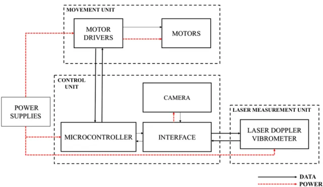
Figure 2.1. System diagram of the proposed device

The system diagram of the offered device is shown in Figure 2.1. The device consists of three separate units. The Laser Doppler Vibrometer (LDV) which is located in the laser measurement unit, allows measuring the vibration of the target surface without any contact. Using the custom graphical user interface (GUI), the points on the target are selected with the help of the acquired camera image which is transferred via the interface. Subsequently, the selected coordinates are transmitted to the microcontroller unit via a serial communication channel. The transmitted data of coordinates determines the information used in detecting the movement of the device. This information controls the motion of the proposed platform with the help of the motor drivers.

(22)

The LDV which is mounted on the proposed measurement device sends the laser beam to the selected point on the target. After that, the measurements are made on the points for a precise amount of time with the help of the motion of the motors shaft. In the next step, the collected data from the chosen points are analyzed using a vibration analysis method and the potential damage on the target is analytically determined.

The creation of the device is planned in two stages. In the first stage, a motorized platform capable of orthogonally moving along two axes is designed. In the second stage, measurements are made while the turbine is parked on the structure with the aid of a LDV placed on this platform.

(23)

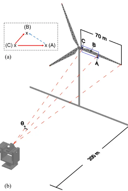
The proposed measurement device determines the amount of change about magnitude for mode shapes on the point of the target in order to identify damages between the decided points. This process is made with the aid of the LDV on the device as shown in Figure 2 (b). For explaining how the device can run through the decided points, the device calculates the angle between the reference point (C) and point A shown in Figure 2 (a). In the next part, these calculated angle values are converted to number of steps by the designed GUI and used microcontroller. At this point, the laser beam travels to a predetermined position thanks to fabricated measurement device. If it is desired that the LDV's laser beam moves from point A to point B, the proposed measurement device first calculates the angle and the number of steps between the B and the center point. It then moves from point A to point B using this information.

The distance between two points on the target is calculated with using the distance of the device to the target and the angle between two points by considering Equation 2.1. The angle of a stepper motor is equal to 1.8 degrees for one step. This angle can be reduced by 1/128. The speed of one step of the device and the measurement period over the selected points on the target can be controlled via the developed GUI.

𝑑_"# =tan𝜃 ∗ 𝑑_* (2.1)

In Equation 2.1., dAB represents the distance between points A and B on the blade shown in Figure 2.2. (b) and dc shows the distance from the measurement device to the target.

𝜃 = 𝑁 ∗ 𝛼 (2.2)

In Equation 2.2., N presents the number of steps of the used motor, and α offers the angle corresponding to one step of the same motor. The scanning area of the measurement device is limited by the angle of the camera placed on the device.

(24)

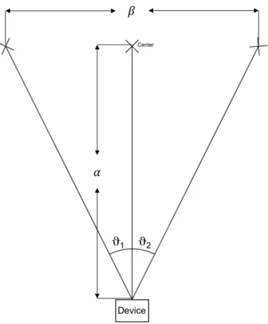
Figure 2.3. Calculation of the scanning area

𝜗_/ = 𝜗₀+ 𝜗₂ = 2 ∗ tan4052

6 (2.3)

Calculation of the scan area depends on field of view of used camera. The scan area can be calculated on the horizontal and vertical axes of the desired device using Equation 2.3 where Jt is the total scan angle of the device for two axes separately, J1 is the angle between start point and center of the target, J2 is the angle between end point and center of the target. Otherwise, β is the length of the target and α is the distance between the laser source and target. In order to calculate the scanning area on the horizontal axis of the device, β and α values are equal to 4640 mm and 5190 mm and the device may scan approximately 48 degrees. On the other hand, β and α values are equal to 2600 mm and 5190 mm for the vertical axes and the device may scan approximately 28 degrees on the vertical axes. The minimum horizontal and vertical scan angle of the system is about 0.014 degrees and this angle completes at 15 milliseconds.

(25)

3. IMPLEMENTATION OF THE SYSTEM

The proposed design consists of two parts. In the first part, mechanical design is mentioned such as dimensions, material, weight, and volume, parts of mechanical design and characteristics of motor that is used. The second part is about software design and explains how the microcontroller works and the custom GUI.

3.1. MECHANICAL DESIGN & FABRICATION

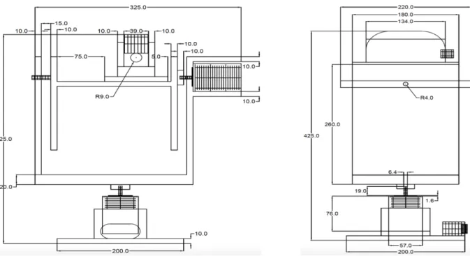
The design has been made by using three-dimensional drawing program in such a way that the movement ability, angle and the precision of the device are optimized in accordance with the LDV's head. The dimension of the mechanical design as shown in the Figure 3.1. These dimensions have been determined by the dimensions of the LDV's head and the sizes of the motors to be placed on the device. The design has been drawn in two dimensions. After that, cutting is done with CNC cutting machine using these drawings. The device is made of plexiglass material because it is desired to be produced at low cost, rapid shaped and easy found material. Moreover, it can provide us to needed mass to make the system stable. The weight of the proposed device is approximately 4 kg and the volume is 0.03 m3.

(26)

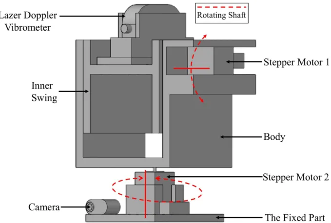
Figure 3.2. Visualize in three-dimension of two-dimensional motorized scanning device

The proposed measurement device that is mechanically completed in three parts as shown in Figure 3.2.; these are the body, the swing on which LDV's head is placed and a fixing part for fixing all of these to the step motor 2. Firstly, a swing is designed to be able to move the vertical axis and fixing the LDV's head. The LDV's head can be carried by slider screw holes in the swing part of the design so that the center of mass of the proposed device can be adjusted. Subsequently, the points at which the position of motor and motor shafts are fixed and determined in the swing and on the body of the device. The rotational shafts of the two motors are designed to be perpendicular to each other. After that, the center of mass of the device is organized by changing the place of sub-equipment that located top of whole device. The parts which are designed separately according to the explanation are assembled as shown in Figure 3.2. Then, the device can be operational and movable. In this way, any desired point within the intended image area can be addressed easily.Figure 3.3. shows the final state of the proposed device.

(27)

(28)

3.2. SOFTWARE DESIGN & IMPLEMENTATION

The software installation has been done for two-dimensional motorized system. In this part, GUI and motor control system are explained.

3.2.1. Graphical User Interface

Figure 3.4. Field of target view

The vertical displacement DY between the starting and target point P can be computed as shown Equation 3.1.

∆𝑌 = 𝐶:− 𝑃: (3.1)

where, Cy represents the coordinate information on the Y-axis of point C and Py represents the coordinate information on the Y-axis of point P.

Whereas the horizontal displacement DX between the starting and target point P can be computed as shown Equation 3.2.

(29)

∆𝑋 = 𝑃>− 𝐶> (3.2)

where, Px represents the coordinate information on the X-axis of point P and Cx represents the coordinate information on the X-axis of point C.

𝑚𝑚_@> = 1000 𝑚𝑚 ∆𝑊 (3.3)

∆𝑊 = 𝐵_>− 𝐴_> (3.4)

𝑚𝑚_@: = 1000 𝑚𝑚 ∆𝐿 (3.5)

∆𝐿 = 𝐸_:− 𝐹_: (3.6)

In the explained above equation, mmpx and mmpy describe millimeter per pixels that introduces how many millimeters can be obtained from one pixel to have the required distance in magnitude of millimeter rather than number of pixel for calculating the angle which will be one of the important step of the Equation 3.8. and 3.9. ∆W defines the change of width which is 1 meter distance on target can be shown in Equation 3.3. Bx and Ax represent x-coordinates of points A and B as shown in Equation 3.4. ∆L corresponds the change of length which is 1 meter distance on target can be shown in Equation 3.5. Ey and Fy represent x-coordinates of points A and B as shown in Equation 3.6.

𝜙

_JK

:

MNO° K_QR

∗

0

02S

(3.7)

“ϕPS” is the angle per step which calculates the one angle for a step, and “SPR” is number of steps per revolution and a constant expression that is 200 and shows us the step number of a tour of motor. However, “ϕPS” can be reduced by the reducing factor of 1/128 to have much tinier angles per a step such 360/200*128.

(30)

𝑉

_𝑠

:

𝑡𝑎𝑛−1 ∆𝑌∗𝑚𝑚𝑝𝑙_𝑑𝑐 𝜙_𝑃𝑆

(3.8)

𝐻

_^

:

/_`ab ∆c∗ddef_gh iQj

(3.9) Vs and Hs are the required step number for traveling any decided distance on vertical axis and horizontal axis, respectively. Besides of all, dc is the distance between laser source of device to target.

Distance of the device to the target, the operating speed of the device and also the distance between the camera located on the device and the target, defined as a data into the developed GUI program. Afterward, first position of the laser upon the device is defined to the GUI and this position is determined as a center. The GUI calculates the distance in pixel by pixel between P point and C point in vertical and horizontal axis for moving the device through P point and the reference point of (C) that showed in Figure 3.4. (can be seen in Equation 3.1 and 3.2.)

These distances are calculated for both axis in millimeters using Equation 3.3 and 3.5. Then the angle of motion of device in both axis can be calculated with using calculated distances by using the Equation 3.8 and 3.9. After the above explained step, these calculated angles used to find number of steps for two axes again by using Equation 3.8. and 3.9. The GUI transmits data that consists needed step information, to micro-controller by using Equation 3.8. and 3.9.

Micro-controller uses this information and decides location of motors and motors drive the device to P point. If it is desired to take measurements from more than one point on the target, firstly the location information of the points to be measured is defined in the user interface memory. Then, it is applied one by one for each point stored in the memory with the above-mentioned method. Thus, the designed device can measure vibration for each selected point on the target and can measure by waiting until the defined analysis period is over.

(31)

Figure 3.5.The block diagram of the working principle of GUI

In order to increase the prototyping speed, Processing tool which is a visual programming language has been used. The window size and the GUI element positions are set by hand. Buttons and Text Fields are created using a GUI library for ease. Some variables, namely Target Distance, Millimeter per Pixel and the Center Position are predefined manually. Target Distance is just the distance of the system to the target in millimeters, the Millimeters per Pixel is measured using the calibration markers on the target, and the Center Position is the position of the laser from the device that camera sees when both axes are parallel to the system. The interface consists of live camera feed, buttons and text fields. If we try to imagine how the interface works, we can arrange the events as follows;

1. Interface initiates with the predefined values and GUI element positions. 2. It waits for a mouse input (mouse click) inside a loop.

3. When a mouse click is received, it gets the X and Y positions of the mouse cursor at the time of clicking.

4. X and Y distance differences in the form of pixels are calculated by subtracting the center position from the clicked position.

(32)

(Y distance difference is the negative of the calculation, because the coordinate system of the computer increases from top to bottom whereas our coordinate system increases from bottom to top).

5. Horizontal and vertical distances are then calculated using these information by multiplying the pixel values by the Millimeters per Pixel constant. This gives us the distances of the selected point from the center point at each axis.

6. Now that we know the vertical and horizontal distance and the distance from device to target, we can calculate the horizontal and vertical angles of the point using the arc-tangent function from mathematics. The operation is simply;

𝜃

_𝑉

= 𝑡𝑎𝑛

−1 ∆𝑌𝑉

𝑑

(3.10) The vertical displacement DYV describes difference between two point and d is the distance between laser source of device to target as shown Equation 3.10.

𝜃

_k

= 𝑡𝑎𝑛

40 ∆l_nm

(3.11) The horizontal displacement DXH describes difference between two point and d is the distance between laser source of device to target as shown Equation 3.11.

This operation gives us the angle differences in each axis of the point compared to the center position of the system.

7. Angle information is then turned into step information by calculating the following formula;

𝐻

_Kk

= 𝜃

_k

∗

KQR

MNO

(3.12)

𝑉

_Ko

= 𝜃

_o

∗

KQR

(33)

HSH and VSV are the step number for moving between two decided points on horizontal axis and vertical axis and SPR is number of steps per revolution as shown in Equation 3.12 and 3.13.

8. Later, the step information is sent to the micro controller via the serial interface to be interpreted and for positioning the motors.

These operations are used to point the system to a single selected point. However, in this project the purpose is to scan multiple points which are spaced evenly. For this, we can simply record the starting and the end points in the memory and then, divide difference of the number of steps to the one less than number of points to be measured. Which can be written as

∆𝑆

_n

=

∆Kgpq

(s_Qt40)

(3.14) where DSd represents step difference for each point and DSdBE represents step difference from beginning to end. Also, NPM defines number of point to be measured.

Later, using the serial interface, we can send the step information of each point sequentially. We can add a delay before sending each point in order to create time for the measurements to be performed.

3.2.2. Motor Control System

In this project, stepper motors were used for accurate and precise positioning. Motors convert electrical energy to mechanical energy. The stepper motor is an electromechanical actuator that converts the input pulse series to an exactly defined movement in the shaft position as a DC motor with lots of teeth acting as smaller stators to increase positioning accuracy. Each pulse that has come from the energy source moving the shaft with a fixed angle movement, called step angle.

(34)

Stepper motors have shown up as cost-effective alternatives for DC motors in high-speed, motion control applications, where the high torque is not required. Stepping motors are generally used in measurement and control applications, such as locating systems for NC machines, some printers, robotics, computer items, automotive devices and small business machines. The Figure 3.5. illustrates the internal view of a typical stepper motor. Stepper motors contain a magnet rotor, coil windings and magnetically conductive stators. When a coil is energized, it creates an electromagnetic field with its poles. The magnetic field can be changed by sequentially energizing the stator coils that generates rotational motion. Thus the stepper motor. Thus, the stepper motors perform the stepping motion [24].

Figure 3.6. The inside of a bipolar stepper motor

In a typical stepper motor, teeth on the rotor side has positioned asymmetrically as seen in the Figure 3.7., so there are more positions for the rotor to be at, again for improved positioning capability by improved sensitivity of the shaft.

(35)

Stepper motors are controlled by the stepper motor drivers in the micro stepping mode and those drivers also control the coil currents and handling all complexity of micro stepping. Thus, the only thing, the microcontroller tells motor drivers whether to step forward or backward and when to do that. The microcontroller also keeps the records of the steps taken and where the motors should be at. That means is that the position of the motors can be determined as desired and the microcontroller can try to establish this position at the desired speed. In simple terms, there is a chaser function in the microcontroller that always tries to match the desired and real positions of each motor at the given speed.

In this project, two high power bipolar stepper motors called NEMA 23 and for driving these motors two AMIS-30543 motor driver circuit have been used. The AMIS-30543 is a micro stepping stepper motor driver for bipolar stepper motors. Input ports of the motor driver circuit are connected to external microcontroller pins and output ports of motor drivers are connected to the stepper motor. This connection made with the serial peripheral interface (SPI). Also, this driver is using a proprietary pulse-width-modulation algorithm for reliable current control. The AMIS-30543 is ideally suited for general purpose stepper motor applications in the automotive, industrial, medical, and marine environment [24].

The image of the NEMA 23 bipolar stepper motor is shown in Figure 3.7. and technical specifications of this stepper motor represented in Table 3.1.

(36)

Table 3.1. Stepper motor technical specifications

Step Angle (°) 1.8˚

Steps per revolution 200

Number of Phase 2

Rated Current (A) 2.8 A per coil Rated Voltage (V) 3.2 V

Resistance Per Phase (W) 1.13 Ω per coil Inductance Per Phase (mH) 3.6 mH per coil

Holding Torque 19 kg-cm

Weight 1.05 kg

Figure 3.9. Driving system diagram for stepper motor

Driving system diagram of the stepper motor presented is shown in Figure 3.8. The direction in which the stepper motors turn can be controlled with the help of microcontroller and motor driver circuit such as the number of revolutions and the rotation speed. Stepper motors are not driven by just connecting the positive and negative leads of the power supply.

(37)

They are driven by a stepping sequence which is generated by a controller. The microcontroller transmits switching signals to the motor driver circuit. Motor driver circuit receives these transmitted signals and transmits the signals to the motor windings through the inputs of the stepper motor. In this way, the stepper motor is moved. Thus, the movement of the shaft of the step motor is provided.

Furthermore, the speed of the stepper motors and the rotation angle of the stepping motor shaft are determined by changing the frequencies applied to their inputs and the ratio of the currents applied to the coils. The stepper motors rotation depends on the number of pulses applied to the inputs. When a single pulse is applied to the input, the rotor moves one step and stops. The motor moves according to described steps above.

The stepper motor has 200 possible positions for a single revolution. Hence the angle for each step is 1.8 degrees as shown in Equation 3.15. However, the motor driver has a function called micro stepping which can improve accuracy even further by adjusting the currents of the stators to make the rotor stay in a kind of half-way position between two teeth.

The excitation current is gradually changed. The current is applied to the first and the second phase is not excited, the motor shaft is in the vertical position. Then gradually the current of the first phase is reduced and the current of the second phase gradually increases. For this reason, the motor shaft will move at a small angle because of this result density of the magnetic field of the first phase and second phase. Thus, increasing the number of steps in a single revolution and making the angle smaller. The general formula for stepping accuracy is shown below.

𝜙

_JK

:

MNO°_K

QR

(3.15) where,

ϕ

PS is the angle per step in degrees, SPR is the number of steps per revolution.

𝑆_Jv = 𝑁_vw∗ 𝜙_xJ

(3.16) where, NRT is the total number of rotor teeth, ϕMP is the number of motor phases.

(38)

The total number of rotor teeth is equal to 100 and the number of motor phases is equal to 2 for our stepper motor. As a result of these equations which are Equation 3.15 and 3.16, the angle corresponding to one step of the motor is equal to 1.8.

Figure 3.10. The block diagram of the working principle of microcontroller

The purpose of the microcontroller in the control system is to get the stepper motors into a desired position with a desired speed and hold them in this position afterwards, unless the computer stated otherwise. The micro controller and the computer are communicating via the serial interface.

(39)

Serial connection is established by a USB connection and a USB to serial converter circuit. Additionally, a specific communication protocol is designed for them to speak together. The micro controller holds the system’s current position an it’s desired position in two 32-bit signed integers (Shown as the Current Position and the Desired Position in the diagram).

Later, this position information is used to move motors to the correct position. If we try to imagine what’s going on in the system when some information has been sent by the computer, we can arrange the events as follows;

1. Computer sends the position information via serial interface using a specific protocol.

2. Micro controller receives this position over the serial port using the same protocol, and it updates the Desired Position according to this information.

3. It repeatedly checks if the Desired Position is smaller or bigger than the Current Position (Current Position is defined as 0 where the device’s both axes are perpendicular to the system).

4. If there is a difference between them, micro controller makes the motors move one step to the necessary direction.

5. It waits at some necessary duration according to the data sent by the computer (while listening the serial at the same time to detect any changes for the Desired Position). 6. It repeats this actions until the Desired Position is equal to the Current Position. After

that, micro controller sends a predefined Position Established signal to the computer via the serial interface.

Additionally, the micro controller also initiates and configures the motor drivers at the beginning.

(40)

4. VIBRATIONAL ANALYSIS

As described in chapter 1, optic measurement methods are used to perform vibration analysis on wind turbines without contact.

4.1. LASER DOPPLER VIBROMETER

A LDV is commonly used in optical methods. LDV can provide very high accuracy (in the range of micron) and spatial resolution and it is a device that is used to make non-contact vibration measurements, determining vibration velocity and displacement on a surface. The operation of the LDV is based on Doppler effect. The Doppler effect is observed whenever the source of the waves is moving according to an observer. The Doppler effect may be defined as the effect produced by a moving source of waves. LDV detects the frequency shifts of the backscattered laser beam due to the motion of the surface. As shown in Figure 4.1., the laser beam splits into two parts; the reference beam is pointed directly to the photo-detector while the measurement beam is incident on the target where the beam is scattered by the moving surface depending on the velocity and displacement. The backscattered beam is changed in frequency and phase the characteristics of the motion are entirely contained in the backscattered beam. This beam with the reference beam creates a modulated detector output signal revealing the Doppler shift in frequency signal processing and analysis provides the vibrational velocity and displacement of the target.

(41)

4.1. POWER SPECTRAL DENSITY

Power Spectral Density (PSD) is the frequency response of a periodic or arbitrary signal. It presents where the average power is distributed as a function of frequency. Power spectral densities (PSD) are used to characterize random vibration signals.

For instance, to characterize a stationary process, an ensemble of time histories must be obtained, wherein the amplitude of time graph is measured according to the frequency range at the excitation. The role of excitations is providing us the reference magnitude of the input that utilized in tests.

Thus, the three related parameters of interest are frequency, time and amplitude. This information can provide the ability to analyze a random process in a statistical approach. In other words, the characterization of random vibration is typically resulted in a frequency spectrum of Power Spectral Density (PSD), which assigns the mean square value of some magnitude that passed by a filter then divided by the bandwidth of the filter. Thus, Power Spectral Density defines the distribution of power over the frequency range of excitation [26-27].

For PSD process, in certain types of random signals is independent of time. This is useful because the Fourier transform of arbitrary time signal has own randomness.

The PSD of a random time signal x(t) can be expressed in one of two ways that are equivalent to each other.

1. The PSD is the average of the Fourier transform magnitude squared, over a large time interval 𝑆_> 𝑓 = lim w→~𝐸 0 2w 𝑥 𝑡 𝑒4•2‚ƒ/𝑑𝑡 w 4w 2

(4.1)

2. Then the power spectral density can be defined as

𝑆 𝜔 = lim

w→∞𝑬 𝑥w 𝜔

(42)

The power spectral density output of wind turbines gives information about mode shapes and possible damage on wind turbines.

4.3. MODE SHAPES OF WIND TURBINES

Mode shapes are special shape functions which show the dynamic vibration patterns of the structure. Since these shapes are obtained by solving the Eigenvalue problem which involves stiffness and mass matrices only, they are not related to the excitation levels and the loads acting on the structure.

For most structures damping is low and can be ignored. If we assume that the system is undamped, for an N degree of freedom system Eigenvalue problem can be stated as follows

𝐾 s>s− 𝜆 𝑀 s>s 𝜙 = 0 (4.3)

The non-trivial solution of this equation requires that the determinant of the expression is zero.

𝑑𝑒𝑡 𝐾 _s>s− 𝜆 𝑀 _s>s = 0 (4.4)

If Equation 4.4 is solved, we get N different λ values which are nothing but the vibration frequencies of N different modes. In Equation 4.5, ω, f and T correspond to angular frequency, frequency and period, respectively.

𝜆 = 𝜔 = 2𝜋𝑓 =

2‚_w

(4.5)

As can be seen from the above mentioned equations, a change observed in modal frequency/period directly shows a change in mass or stiffness matrices and therefore can be attributed to the existence of a structural damage.

(43)

Although frequency shifts are very important damage indicators they cannot provide any information related to the extent and location of the damage. This information can be acquired from mode shapes. If the mode shapes of the healthy (reference) and damaged structures are compared, the location of the damage can be determined. Similarly, if the Finite Element Model of the structure exists, it can be analyzed for different damage levels to find what kind of damage causes the observed change in the mode shape. The success of all these steps is directly related to how accurate the mode shapes can be extracted. Damage detection, determination of the location and the extent of the structural damage is beyond the scope of this work; however, it should be shown that mode shapes can be determined with sufficient spatial accuracy. Indeed, this is the most important advantage of using a LDV because unlike accelerometers or piezoelectric or fiber optic strain gauges, in laser vibrometer measurements data points are not limited, therefore even very small stiffness degradations can be determined with high accuracy.

Mode shapes can be calculated by modal decomposition of the real vibration measurements. During the vibration tests, the magnitude of the forces may vary which results in a change in the magnitude of the measured vibrations. However, if there exists a fixed location reference measurement, the ratio of the magnitude of modal amplitude of a random measurement location to the modal magnitude of the reference signal can be used to eliminate the effect of excitation. Therefore, at least one reference signal is required to combine the vibration data coming from different measurements during which the excitation levels may differ. In this work as reference sensor we used an accelerometer which is located at a fixed point. As the moving sensor LDV was used to take several measurements on the blade.

There are numerous methods for modal decomposition, in this work we use a frequency domain analysis method and the ratio of the PSD (Power Spectral Density) magnitudes coming from different data series. This method can also be seen in the figure below. If 4 different measurements are taken on the system, by combining the magnitudes of the peaks seen in PSD graphs, the mode shapes shown on the left can be obtained.

(44)

(45)

5. EXPERIMENTAL RESULTS

This chapter aims at describing the main features of the vibration tests performed on a small-scale wind turbine model by using a motorized system and the GUI developed.

The measurement point can be selected on the target surface with the aid of the GUI shown in Fig. 5.1. and the device can be made available to measure the vibration on the surface. Measurement device automatically decides where to go based on the starting point. Subsequently, the points to be measured on the target are determined by means of the developed interface program as indicated in Fig. 5.1. Finally, the data are collected from the determined points on the target and vibration analysis is done by using these data with the help of LDV.

Figure 5.1. Reference and measurement points of determined on GUI

First, the measurement points are selected via the GUI. When the "Go Next Point or Go Sequentially" button on the GUI is clicked, the laser beam of the LDV on the proposed device comes to the first point of the selected target and the necessary data is obtained for vibration analysis on the point as seen Fig. 5.4. In this way, a vibration analysis is performed for each selected point on the target respectively and the health status of the structure is determined.

(46)

The proposed device can also work in another way. It can equally divide the line drawn between the two points selected on the target. In order to do this, the start and end points are selected and stored in memory as seen in Fig. 5.2. Then the number of measuring points is saved in the system and the device moves to the points sequentially between start and end points where the measurement is performed as shown in Fig. 5.3. In this way, a vibration analysis is applied for each selected point and data for vibration analysis is obtained on the point as seen Fig. 5.4.

Figure 5.2. Start and end points which are selected with red dot in GUI

(47)

(48)

Vibration measurements were taken with the help of motorized LDV on the points shown in Fig. 5.1. The obtained data were taken and stored by using an oscilloscope and then imported to MATLAB. They were mapped in the frequency domain using the PSD method described in the previous chapter. The obtained vibration data are given in Figure 5.5 from the wind turbine model which is designed for tests.

In the graphs, the y-axis and x-axis represent the PSD amplitude and the frequency, respectively. These analyses are performed for all the points on the blade and stored in a database. Vibration data extracted from different measurements are combined by scaling all the data with respect to the reference in frequency domain.

If there is a crack or damage on the turbine surface, due to the increase in flexibility, the frequency will be shifted to the left. In other word, it will be decreased. Also, the ratio of the PSD magnitudes obtained at different locations will change. In the figures shown below the first peak at 2.69 Hz corresponds to the first flap wise (out of plane direction) mode of the blade. Similarly, the second peak at 4.52 Hz is related to the 2nd mode in flap wise direction. The 3rd mode at 6.17 Hz is 1st bending mode of the tower in fore-aft direction. Since the frequency resolution of the PSD plots is 0.1 Hz some deviations in frequency can be observed but the calculated frequencies are stable and can be clearly seen on each plot.

(49)

Figure 5.5. Power spectral density graph of tip displacement on the blade (First Peak - Frequency: 2.689 / Amplitude: 657.1, Second Peak - Frequency: 4.595 / Amplitude: 46.34, Third Peak – Frequency: 6.214 /

Amplitude: 20.46)

Figure 5.6. Power spectral density graph of mid-point displacement on the blade (First Peak - Frequency: 2.709 / Amplitude: 232.9, Second Peak - Frequency: 4.522 / Amplitude: 53.54, Third Peak – Frequency:

(50)

Figure 5.7. Power spectral density graph of nacelle displacement (First Peak - Frequency: 2.682 / Amplitude: 161.1, Second Peak - Frequency: 6.174 / Amplitude: 13.32)

(51)

6. CONCLUSION AND FUTURE WORK

In this study, a novel automated laser scanning system with 2D motorized device that can move with two axes is realized. Thanks to the advanced optical measurement techniques the time-lapse cracks and damage on the wind turbines could be observed without causing more loss. Observations have been made on the dynamic response of wind turbines to determine how to remove negative influences such as cracks and fractures. For this purpose, a device capable of motion and measurement at the same time is designed and manufactured. In addition to this, a GUI has been developed to control this device.

The experimental results also confirm that the presented 2D motorized device can be utilized. The device may scan approximately 48 degrees on the horizontal axis and 28 degrees on the vertical axis. The minimum horizontal and vertical scan angle of the device is obtained 0.014 degrees. The minimum scan angle completion time is 15 milliseconds. The volume of device is measured as 0.03 m3 and weight of device is measured as 4 kg. The operating power of device is calculated as 12 Watt.

It is aimed to determine the potential problems by means of this measurement system and thus to determine and prevent micron scale damage. Vibration analysis was performed with the wind turbine model which is specially designed by the LDV which is placed on the device. Based on the analysis, the modal data of a blades of the wind turbine model is reached.

In the future work, a new device will be fabricated in aluminum material in order to eliminate its errors and develop its operation. The horizontal and vertical scan angle will be increased for more sensitivity and an infrared laser will be placed on the device so that there will be no need for additional reflective markers on the target surface. In addition, this device has been built for mobile targets, but now it is working on static targets. The newly developed device was designed with AutoCAD as software and it is planned to work on mobile targets which is seen in Figure 6.1.

(52)

(53)

APPENDIX A: 2D Drawings, CNC Cutter Machine and Parts of Device

(54)

(55)

Figure A.3. The cutting process was photographed, it was performed with CNC cutter machine

(56)

Figure A.5. Photos of body and motor

(57)

REFERENCES

[1] H. Larsen and L. S. Petersen, "The Future Energy System Distributed Production and Use," Riso National Laboratory, Denmark, 2005. [2] M. Ozbek, D. J. Rixen, O. Erne and G. Sanow, "Feasibility of monitoring large wind turbines using photogrammetry," Journal of Energy, vol. 35, p. 4802–4811, 2010.

[3] G. H. James, T. G. Carne and J. P. Lauffer, "Modal testing using natural excitation," in

Proceedings of the 10th International Modal Analysis Conference, San Diego, California, 1992. [4] D. J. Malcolm, "Dynamic response of a Darrieus rotor wind turbine subject to turbulent flow," Engineering Structures 10, pp. 125-134, 1988. [5] D. T. Griffith, R. L. Mayes and P. S. Hunter, "Excitation methods for a 60 kW vertical axis wind turbine," in Proceedings of the 28th International Modal Analysis Conference, Jacksonville, Florida, USA, 2010. [6] D. J. Malcolm, "Structural response of 34-m Darrieus rotor to turbulent winds," Journal of Aerospace Engineering, vol. 6, pp. 55-75, 1993. [7] T. G. Carne, J. P. Lauffer and A. J. Gomez, "Modal testing of a very flexible 110m wind turbine structure," in Proceedings of the 6th International Modal Analysis Conference, Kissimmee, Florida, USA, 1988. [8] M. H. Hansen, K. Thomsen and P. Fuglsang, "Two methods for estimating aeroelastic damping of operational wind turbine modes from experiments," Wind Energy 9, pp. 179-191, 2006. [9] D. P. Molenaar, "Experimental modal analysis of a 750 kW wind turbine for structural model validation," in Procedings of the 41st Aerospace Sciences Meeting and Exhibit, Reno, Nevada, 2003. [10] R. Osgood, G. Bir, H. Mutha , B. Peeters and M. Luczak, "Full-scale modal wind turbine tests: comparing shaker excitation with wind excitation," in Proceedings of the 28th International Modal Analysis Conference, Jacksonville, Florida, USA, 2010.

(58)

[11] T. C. J. L. G.H. James, "The natural excitation technique (NExT) for modal parameter extraction from operating wind turbines, Technical Report," Sandia National Laboratories, 1993. [12] M. Ozbek and D. J. Rixen, "Operational Modal Analysis of a 2.5 MW Wind Turbine Using

Optical Measurement Techniques and Strain Gauges," Wind Energy, vol. 16, pp. 367-381, 2013. [13] M. Ozbek , F. Meng and D. J. Rixen, "Challenges in Testing and Monitoring the In-Operation Vibration Characteristics of Wind Turbines," MSSP Mechanical Systems and Signal Processing, vol. 41, p. 649-666, 2013. [14] J. S. G.P. Corten, "Optical motion analysis of wind turbines," in Delft University of Technology, SV Research Group, 1995. [15] G. P. Corten, "Optical Motion analysis of wind turbines," in Proccedings of European Union Wind Energy Conference, Bedford UK, 1996.

[16] Y. Tamura , M. Matsui, L. C. Pagnini, R. Ishibashi and A. Yoshida, "Measurement of wind-induced response of buildings using RTK-GPS," Journal of Wind Engineering Industrial

Aerodynamics 90, p. 1783–1793, 2002.

[17] S. Nakamura, "GPS measurement of wind-induced suspension bridge girder displacements,"

ASCE Journal of Structural Engineering 126 (12), p. 1413–1419, 2000.

[18] P. Breuer, T. Chmielewski, P. Gorski and E. Konopka, "Application of GPS technology to measurements of displacements of high-rise structures due to weak winds," Journal of Wind

Engineering and Industrial Aerodynamics 90 (3), p. 223–230, 2002.

[19] A. Nickitopoulou, K. Protopsalti and S. Stiros, "Monitoring dynamic and quasi-static deformations of large flexible engineering structures with GPS: Accuracy, limitations and promises," Engineering Structures 28, pp. 1471-1482, 2006.

[20] L. W. M.M. Rademakers, T. W. Verbruggen, P. A. van der Werff, H. Korterink, D. Richon, P. Rey and F. Lancon, "Fiber optic blade monitoring," in European Wind Energy Conference, London, 2004.

(59)

[21] K. Schroeder, W. Ecke, J. Apitz, E. Lembke and G. Lenschow, "A fiber Bragg grating sensor system monitors operational load in a wind turbine rotor blade," Measurement Science and Technology, 17, p. 1167-1172, 2006. [22] E. M. Mikhail, J. S. Bethel and J. C. McGlone, Introduction to modern photogrammetry, New York: Wiley & Sons, 2001. [23] S. Yang and M. S. Allen, "Output-only Modal Analysis using Continuous-Scan Laser Doppler Vibrometry and application to a 20 kW wind turbine," Mechanical Systems and Signal

Processing, vol. 31, p. 228–245, 2012.

[24] D. Samokhvalov, S. Stoliarov and A. Kekkonen, "The Hybrid Stepper Motor Modeling in Simulink," in Young Researchers in Electrical and Electronic Engineering Conference

(EIConRusNW), Russia, 2015.

[25] onsemi.com, "AMIS-30543/Micro-Stepping Motor Driver," 2014. [Online]. Available: http://www.onsemi.com/pub/Collateral/AMIS-30543-D.PDF . [Accessed 2017].

[26] A. V. Oppenheim, A. S. Willsky and S. H. Nawab, Signals & Systems, New Jersey: Prentice Hall, 1997.

[27] A. V. Oppenheim and R. W. Schafer, Discrete-Time Signal Processing, New Jersey: Prentice Hall, 1989.