Feedback Adaptive Learning for Medical and
Educational Application Recommendation
Cem Tekin, Senior Member, IEEE, Sepehr Elahi, Student Member, IEEE, Mihaela van der
Schaar, Fellow, IEEE
Abstract—Recommending applications (apps) to improve health or educational outcomes requires long-term planning and adaptation based on the user feedback, as it is imperative to recommend the right app at the right time to improve engagement and benefit. We model the challenging task of app recommendation for these specific categories of apps—or alike—using a new reinforcement learning method referred to as episodic multi-armed bandit (eMAB). In eMAB, the learner recommends apps to individual users and observes their interactions with the recommendations on a weekly basis. It then uses this data to maximize the total payoff of all users by learning to recommend specific apps. Since computing the optimal recommendation sequence is intractable, as a benchmark, we define an oracle that sequentially recommends apps to maximize the expected immediate gain. Then, we propose our online learning algorithm, named FeedBack Adaptive Learning (FeedBAL), and prove that its regret with respect to the benchmark increases logarithmically in expectation. We demonstrate the effectiveness of FeedBAL on recommending mental health apps based on data from an app suite and show that it results in a substantial increase in the number of app sessions compared with episodic versions of
✏n-greedy, Thompson sampling, and collaborative filtering methods.
Index Terms—Recommender systems, application recommendation, online learning, multi-armed bandit.
F
1 I
NTRODUCTIONA
S the use of mobile devices in everyday life keeps growing at an unprecedented rate, there has been a surge of mobile applications that affects various aspects of modern life such as personalized healthcare, education, and entertainment services. Choosing the applications that match with the needs of the users from a large and diverse set of alternatives requires development of sophisticated recommendation methods [1], [2], [3], [4]. In order to achieve a high level of personalization in this diverse environment, application stores have adopted taxonomy based categoriza-tion of the apps [5]. Therefore, to achieve optimal personal-ization, category specific challenges of user-app interaction need to be taken into account when designing recommen-dation algorithms.Recently, there has been a growing interest in two spe-cific app categories, namely medical [6] and educational [7] apps. App recommendations for both of these categories are goal driven, i.e., recommendations are made with the goal of improving health or educational outcomes. Therefore, what to recommend and when to recommend should be carefully chosen based on the past feedback from the users in order to align the sequence of recommendations with the ultimate goal. In this paper, we address this task by proposing a new learning framework for feedback adaptive app recommendation.
We start by explaining why medical and educational app recommendation require feedback adaptive learning by providing a set of real-world examples. For instance, a suite of apps with educational and interactional style C. Tekin and S. Elahi are with the Department of Electrical and Electronics Engineering, Bilkent University, Ankara, Turkey. Email: [email protected], [email protected]. M. van der Schaar is with the Department of Applied Mathematics & Theoretical Physics, University of Cambridge, Cambridge, UK. Email: [email protected].
to support users to acquire a set of skills of managing depression or anxiety is considered in IntelliCare [8]. The goal of this study was to observe user interactions with apps and improve users’ conditions by randomly recommending apps so that by analyzing the user data, a recommendation engine could be developed. Improving a user’s condition is challenging because it is difficult to asses the improvement in the patient’s condition due to app recommendations. However, the patient’s interactions with the apps, including time spent in an app, number of times an app is opened etc. (collectively referred to as user engagement), provide aux-iliary information about patient outcomes, and thus can be used as a proxy to the benefit that the patient receives from the apps. Therefore, the efficiency of app recommendations can be measured by user engagement.
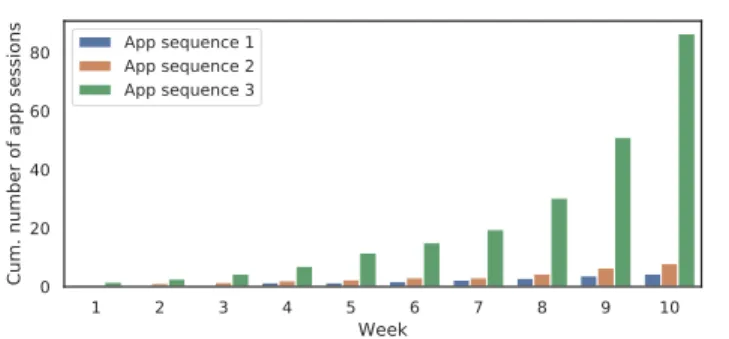
In this setting, the order of app recommendations play a central role in improving user engagement [9]. Moreover, further app recommendations are driven by current user en-gagement. Back to our example of medical app recommen-dations: when users participating in the IntelliCare exper-iment were recommended the same mental-illness-aiding apps each week but in different orders, their engagement vastly varied. Fig. 1 shows the cumulative number of app sessions that an average user had when recommended three different sequences of apps from a set of five different apps, for ten weeks. Notice that the “right” sequence results in more than four times the number of total app sessions than the next best sequence by the end of the tenth week. This example demonstrates the importance of recommending the right app at the right time.
Besides medical apps, educational apps for learning lan-guages have also shown to be very effective and popular [10]. Notice that it makes sense to recommend different educational apps at different time steps (weeks), because
IEEE TRANSACTIONS ON SERVICES COMPUTING 2
some apps are geared to beginners whereas others are made for intermediate or advanced learners. For instance, it would be better to recommend a simple app that teaches basic English words, like Duolingo1, to an English learner who
is just starting out. As this learner practices and improves his English skills (i.e., time passes), he can be recommended a more advanced app like Grammarly2that checks the tone
of an essay.
Both of the examples discussed above motivate us to model app recommendations as a structured reinforcement learning problem called episodic multi-armed bandit (eMAB). In eMAB, the learner proceeds in episodes ⇢ = 1, 2, . . . (users arriving sequentially over time)3 composed of
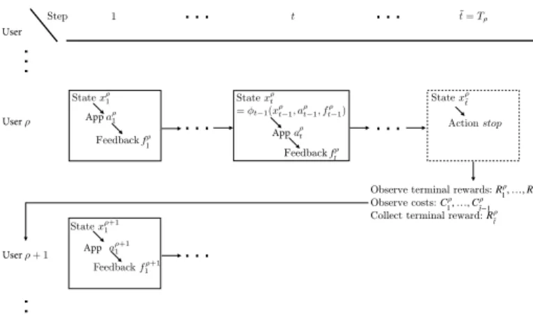
mul-tiple steps (weeks), in which the learner selects actions (app recommendations) sequentially in steps, one after another, with each action belonging to the action set A. After each taken action a 2 A, a feedback f 2 F (number of app sessions in the week after the app recommendation) is observed. Based on all its previous observations in that episode, the learner either decides to continue to the next step by selecting another action or selecting a stop ac-tion (stop app recommendaac-tions) which ends the current episode, yields a terminal reward (total number of app sessions), and starts the next episode. Hence, the number of steps in each episode is a decision variable, and the terminal rewards and costs of the steps in an episode are observed only after the stop action is taken. The goal of the learner is to maximize its total expected gain (i.e., the terminal reward minus costs) over all episodes by learning to choose the best action sequence given the feedback. An illustration that shows the order of steps, costs, terminal rewards and episodes for app recommendation is given in Fig. 2.
In short, we depart from the prior work in recommender systems [11], [12], [13] by modeling the long-term inter-action between the users and the system as a MAB. In particular, in medical application recommendation: (i) Users start using an application suite usually after a diagnosis; (ii) Continuously recommending applications to a user may have negative impact and result in user disengagement, thus one should stop recommendations after some time when the cost exceeds the future benefit; (iii) Users stop using the application suite when the treatment ends.4 The
learner does not know when a user should stop at the beginning, since when to stop should be adjusted based on the improvement in user’s medical condition and user engagement, which can only be inferred from user feedback.
1. www.duolingo.com 2. www.grammarly.com
3. Our model can easily be adapted to handle batch user arrivals or new users arriving before the current user completes its episode. However, for the clarity of presentation and technical analysis, and to remove the potential bias that the user arrival process might have on the performance, we assume throughout the paper that users arrive se-quentially over time. Batch arrivals are considered in the experimental results.
4. Educational application recommendations follow a similar trend: (i) Users start using an application suite/bundle to learn a subject, e.g., a language, up to a certain level; (ii) Level of recommended applications should match level of the user; otherwise the user may lose interest and drop out; (iii) Users stop using the application suite when they gain the expected level of expertise on the subject. Note that in cases where apps are to be recommended indefinitely, the stop action can be removed from the action set without any detriment to recommendation performance.
Fig. 1: The cumulative number of app sessions that a user in the IntelliCare experiment had when recommended three different sequences containing the same five apps.
In general, users can drop out of the system if they are unsatisfied with the recommendations. Thus, it might be beneficial to stop when we are confident that the remain-ing app recommendations will not provide future benefit. In addition, recommendations may have a monetary cost in many settings. Since the number of apps a user can simultaneously use is limited, recommendations can have a diminishing return over time. For instance, a user who is already satisfied with the apps that he/she is currently using, will have little incentive to download and use a new app.
The contributions are summarized as follows:
• We model app recommendations as a structured
reinforcement learning problem called eMAB.
• We propose the FeedBack Adaptive Learning
(Feed-BAL) and compare FeedBAL with a benchmark that always chooses the myopic best action given the current feedback, and prove that it achieves O(log n) regret, where n denotes the number of episodes. Moreover, the regret has polynomial dependence on the number of steps, actions and states. This result also indicates that the difference between the average performance of FeedBAL and that of the benchmark diminishes at a rate O(log n/n).
• We use FeedBAL for recommending mental health
apps based on real data from an app suite, and prove that it significantly improves user engagement. The rest of the paper is organized as follows: Related works are given in Section 2, mathematical descriptions of eMAB, benchmark and the regret are given in Section 3, description of FeedBAL and its regret are given in Section 4, regret bounds of FeedBAL are given in Section 5, FeedBAL’s effect on user engagement in medical app recommendation is given in Section 6, and finally concluding remarks are given in Section 7. Additionally, proofs are given in the supplemental document.
2 R
ELATEDW
ORKSMatrix Factorization: Matrix factorization methods have
been extensively used for making personalized app rec-ommendations. For instance, a method that mines context-aware user preferences from context logs is proposed in [11]. In order to deal with sparse and binary user-app interaction feedback, a method that performs kernel-incorporated ma-trix factorization is developed in [13]. In addition to these,
[12] addresses the problem of predicting users’ preferences for apps using factorization machines. All of the works mentioned above require a priori data to train their models. In contrast, our model is completely online. It uses data gathered from the previous users to inform app recommen-dations for the current user. As the data gathering process is tied with the recommendation process, it is necessary to balance exploration and exploitation. Indeed, we are able to quantize how the accuracy of our recommendations im-prove as more data is gathered (Theorem 1, 2 and Corollary 1, 2) by judiciously balancing exploration and exploitation.
Adaptive Treatment Strategies: Mobile apps have also
been used for treating patients. There has been a surge of research on developing machine learning methods of esti-mating optimal treatment regimes to assign interventions or recommendations to patients. A dynamic programming based method using backward induction [14] and a struc-tural nested mean method with G estimation [15] have laid a foundation for estimating a sequence of decision rules to optimize a long term health outcome. Based on the backward induction framework, the most commonly used methods to estimate optimal treatment regimes are Q(uality) learning [9], [16] and A(dvantage) learning [17], [18]. Q learning is a basic reinforcement learning method to model the cumulative reward conditioning on the state and action, while A learning models the contrast of cumulative reward under different actions.
MABs: eMAB is related to various existing classes of
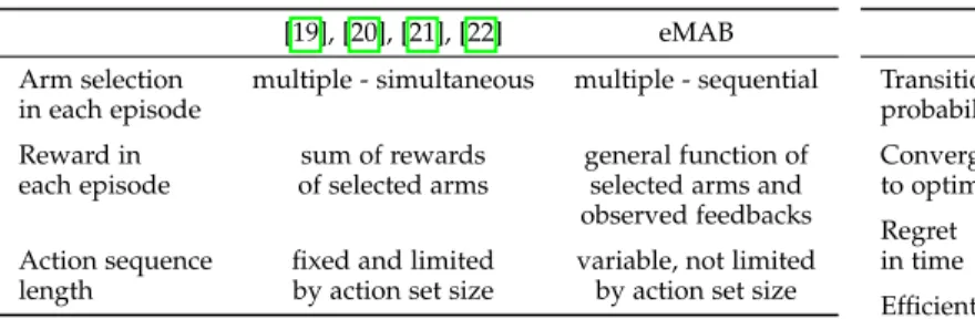
MAB with large action sets. These include combinatorial bandits [19], [20], [21] and matroid bandits [22]. In these works, at each time, the learner (simultaneously) chooses an action tuple and obtains a reward that is a function of the chosen action tuple. Unlike these works, in eMAB actions in an episode are chosen sequentially, and the previously chosen actions in an episode guide the action selection process within that episode. The differences between eMAB and these various classes of MAB are given in Table 1a.
One of the most closely related prior works is the work on adaptive submodularity [23] where it is shown that for adaptive submodular reward functions, a simple adaptive greedy policy (which resembles our benchmark) is 1 1/e approximately optimal. Hence, any learning algorithm that has sublinear regret with respect to the greedy policy is guaranteed to be approximately optimal. This work is ex-tended to an online setting in [24], where prior distribution over the state is unknown and only the reward of the chosen sequence of actions is observed. However, an independence assumption is imposed over action states to estimate the prior in a fast manner.
Markov Decision Processes (MDPs): Our problem is
also related to reinforcement learning in MDPs. For instance, in [25] and [26] algorithms with logarithmic regret with respect to the optimal policy are derived for finite, recurrent MDPs. However, the proposed algorithms rely on vari-ants of value iteration or linear programming, and hence, have higher computational complexity than our proposed method. Episodic MDPs are studied in [27], and sublinear regret bounds are derived assuming that the loss sequence is generated by an adversary. eMAB differs from these works as follows: (i) The number of visited steps (states) in each episode is not fixed; (ii) During an episode, only feedbacks
are observed and no reward observations are available for the intermediate states; (iii) Rewards of the intermediate states are only revealed at the end of the episode. Recently, improved gap-independent regret bounds are derived for reinforcement learning in MDPs by using an optimistic ver-sion of value iteration [28] for episodic MDPs and posterior sampling for non-episodic MDPs [29]. While it is possible to translate eMAB into an MDP, finding the optimal policy in the MDP is more challenging than competing with our benchmark, both in terms of the speed of learning and cost of computation. Thus, eMAB can be seen as a bridge be-tween standard MAB and reinforcement learning in MDPs, where the order of actions taken in each episode matters and the learner aims to perform as good as a moderate benchmark which may not always be optimal, but outperforms the best fixed action and works well in a wide range of settings.
In [30], PAC bounds are derived for continuous state MDPs with unknown but deterministic state transitions and geometrically discounted rewards, using a metric called policy-mistake count. In contrast, we develop regret bounds for eMAB which hold uniformly over time for unknown, random state transitions, and undiscounted rewards. We would also like to note that, model-free methods like Q-learning [31] and TD( ) [32] will be highly inefficient due to the size of the sequence of actions that can be taken, and the sequence of feedbacks that can be observed in each episode. In contrast, regret of eMAB depends only polynomially on the episode length and logarithmically on the number of episodes.
The differences between eMAB, and optimization and reinforcement learning algorithms for MDPs are given in Table 1b.
3 P
ROBLEMF
ORMULATIONNotation: Sets are denoted by calligraphic letters, vectors
are denoted by boldface letters and random variables are denoted by capital letters. For a set E, SE := |E|, where
| · | denotes the cardinality. The set of positive integers up to integer t is denoted by [t]. Ep[·] denotes the expectation
with respect to probability distribution p. I(E) denotes the indicator function of event E which is one if E is true and 0 otherwise. For a set E, (E) denotes the set of probability distributions over E. All inequalities that involve random variables hold with probability one.
Background on Reinforcement Learning and MAB:
Re-inforcement learning can be used to model the long-term interaction between the user and the system [32] in ap-plication recommendation. Within this context, user has a state xt which is affected by the recommendation actions
at chosen by the system. The user responds to the chosen
action by generating a stochastic feedback ft and by
tran-sitioning into a new state xt+1. The goal is to maximize
the expected cumulative feedback E[Ptft] (or expected
discounted cumulative feedback), without knowing a priori stochastic dynamics of the system. Popular reinforcement learning methods include Q-learning and SARSA [32].
Standard MAB [33] can be viewed as a reinforcement learning problem where the state xtis fixed and does not
evolve based on the chosen actions. Compared to general reinforcement learning, this simplification allows derivation
IEEE TRANSACTIONS ON SERVICES COMPUTING 4
TABLE 1: Comparison of eMAB with
(a) combinatorial and matroid bandits.
[19], [20], [21], [22] eMAB Arm selection multiple - simultaneous multiple - sequential in each episode
Reward in sum of rewards general function of each episode of selected arms selected arms and observed feedbacks Action sequence fixed and limited variable, not limited length by action set size by action set size
(b) optimization and reinforcement learning algorithms.
PI, VI Q-learning, TD( ) eMAB
Transition known unknown unknown
probabilities
Convergence always may converge converges to optimal optimal asymptotically asymptotically
Regret zero may be logarithmic
in time sublinear
Efficient for small action small action large action sequences sequences sequences
of much sharper performance guarantees for the standard MAB, namely regret bounds. As the feedback depends on the chosen action, the goal is to maximize the expected cu-mulative feedback E[Ptft]without knowing arm feedback
distributions beforehand. The optimal policy in the standard MAB is the one that always picks the action with the highest expected feedback. The regret is the difference between the expected cumulative feedback of the optimal policy and that of the learning policy. Since the optimal policy is unknown, one needs to tradeoff exploration and exploitation in order to maximize E[Ptft], which is equivalent to minimizing
the regret. Popular algorithms for MAB include upper con-fidence bound based optimistic exploration algorithms [34] and Thompson sampling [35]. It is known that the regret of these algorithms scale as O(log t) in time. This means that the gap between their average feedback and that of the optimal policy diminishes at rate O(log t/t).
As we will describe in the following subsection, our model is much more intricate than a standard MAB. Unlike a standard MAB, we allow the user’s state to evolve over time. Moreover, our model allows maximization of a more general set of performance indicators. At the same time, we are able to obtain sharp performance guarantees for the algorithm that we propose.
Problem Description: The system proceeds in episodes
indexed by ⇢. Each episode represents interaction of the system with a particular user, and is composed of multiple steps indexed by t. In each step the system takes an action from a finite set of actions denoted by ¯A. There are two types of actions in ¯A: (i) recommendation actions which move the system to the next step and allow it to acquire more information (feedback), (ii) termination action (also named as the stop action) which ends the current episode and yields a terminal reward.
Our mathematical model assumes that users arrive one after another, thus, the episode of a new user begins only after the episode of the current user ends. This assumption allows us to clearly quantize the amount of information learned from previous episodes, thereby leading to sharp performance bounds characterized in terms of the regret of learning. In reality, users presence might overlap in time. This is exactly what we consider in simulations (Section 6).
The set of recommendation actions is denoted by A. The maximum number of steps in an episode is lmax<1, which
implies that the stop action must be selected in at most lmax
steps. After an action a 2 A is selected in a step t, the learner observes a feedback f 2 F before moving to the next step,
where F denotes the set of all feedbacks. In the context of application recommendation, feedback can be the indicator of downloading the application, rating, or usage statistics such as number of app sessions.
Let a[t] := (a1, a2, . . . , at)denote a length t sequence of
recommendation actions and f[t] := (f1, f2, . . . , ft)denote
a length t sequence of feedbacks. Let At:=Qt
i=1A denote
the set of length t sequences of recommendation actions and Ft := Qt
i=1F denote the set of length t sequences
of feedbacks. Set of all recommendation action sequences is denoted by Aall := Slmax 1
t=1 At and the set of all feedback
sequences is denoted by Fall := Slmax 1
t=1 Ft. At each step,
the system is in one of the finitely many states, where the set of states is denoted by X . State of the system can be interpreted as a summary of the past interaction of the user with the system. It can be viewed as endogenous contextual information of the user. It is composed of components that are extracted from application usage data. For instance, it can include cumulative number of app sessions, application specific regularity in usage [36] and average rating given to all apps in the system by the user so far.
When action a is chosen in step t, the feedback it generates depends on the state of the system in that step. Specifically, we assume that ft ⇠ pt,x,a 2 (F), where
pt,x,a denotes the probability distribution of the feedback
given the step-state-action triplet (t, x, a). Randomness of the feedback captures the uncertainty due to unobserved variables that govern the interaction between the users and the system. Importantly, we consider the challenging case where pt,x,a is unknown. Let t : X ⇥ A ⇥ F ! X
be the state transition function which encodes every state-action-feedback triplet to one of the states in X . Since the feedback is random, the next state is not a deterministic function of the previous state. Moreover, the state transition probabilities are step dependent.
The expected cost of recommendation a in step t when the state is x is given by ct,x,a 2 [0, cmax]. Cost can be the
difficulty level of the app (some apps can be more challeng-ing than the others so that the user needs to gain experience from the other apps before he/she can benefit from this particular app) or the cost of recommendation due to ad placement (text recommendation, video recommendation, etc.) The expected terminal reward in step t when the state is x is given by rt,x 2 [0, rmax]. This could represent the
average rating, the click probability, or the total number of app sessions. The ex-ante terminal reward of the triplet
…
…
…
…
a1 ⇢ State x⇢ 1 State x⇢t = t 1(x⇢ t 1, a⇢t 1, f⇢t 1) a⇢t…
Action stop…
t 1 State x⇢+1 1 a1 ⇢+1 Feedback f⇢+1 1…
˜ t = T⇢ State x⇢ ˜ t ⇢ + 1 ⇢ Step Feedback f1 Feedback ftObserve terminal rewards: Observe costs: Collect terminal reward:
R1, …, R˜t
C1, …, C˜t 1 R˜t
Fig. 2: x⇢
t is the state observed, a ⇢
t is the action selected and
ft⇢is the feedback observed in the step t of episode ⇢. Ct⇢is
the cost of selecting action a⇢ t and R
⇢
t is the terminal reward
in step t of episode ⇢. T⇢ is the step in which the learner
(system) selects the stop action after which the costs and terminal rewards are revealed.
(t, x, a)is defined as yt,x,a:= E[rt+1, t(x,a,ft)]which gives
the expected terminal reward of stopping at step t + 1 after choosing action a in step t and before observing the feedback ft. For the stop action the cost is always zero
and yt,x,stop = rt,x, 8t 2 [lmax], 8x 2 X . The gain of an
action a 2 ¯A in step t when the state is x is defined as gt,x,a:= yt,x,a ct,x,a.
At each episode ⇢, the system chooses a sequence of ac-tions a⇢:= (a⇢
1, . . . , a ⇢
T⇢), observes a sequence of feedbacks
f⇢ := (f1⇢, . . . , fT⇢⇢ 1)and encounters a sequence of states x⇢:= (x⇢
1, . . . , x ⇢
T⇢), where T⇢denotes the step in which the
stopaction is taken. Since no feedback is present in the first step, for simplicity we set x⇢
1 = 0. In principle, the system
can work with different initial states x⇢
1 2 X . We note
that our model allows us to capture exogenous contextual information about the user through the initial state x⇢
1. After
the stop action is taken, the system observes costs of the selected actions C⇢
t = ct,x⇢t,a ⇢
t + ⌘
⇢
t for t 2 [T⇢ 1]and the
terminal rewards R⇢
t = rt,x⇢t +
⇢
t for t 2 [T⇢], where ⌘⇢t
and ⇢
t are independent -sub-Gaussian random variables
that are also independent from x⇢ 1:t, a ⇢ 1:t, f ⇢ 1:t, ⇢ 1:t 1, ⌘ ⇢ 1:t 1, i.e., 8 2 R and ✓⇢ t 2 {⌘ ⇢ t, ⇢ t}, E[e ✓ ⇢ t] exp ⇣ 2 2 2 ⌘ . When the episode is clear from the context, we will drop the superscripts from the expressions above.
We assume that the state transition function is known and the state of the system can be computed at any step by using the actions taken and feedbacks observed in the previous steps. Feedback, cost and terminal reward distribu-tions are unknown beforehand. The goal is to maximize its cumulative gain over the episodes by repeated interaction with the system (Fig. 2).
The Benchmark: Since the number of possible action and
feedback sequences is exponential in lmax, it is very
inef-ficient to learn the best action sequence by separately esti-mating the expected gain of each action sequence a 2 Aall.
In this section we propose a (greedy) benchmark, given in Algorithm 1, whose action selection strategy can be learned quickly.
The benchmark5 incrementally selects the next action
based on the past sequence of feedbacks and actions. If the stopaction is not taken up to step t, the benchmark selects its action in step t according to the following rule: Assume that the state in step t is x. If gt,x,stop gt,x,afor all a 2 A
(which implies that rt,x yt,x,a ct,x,afor all a 2 A), then
the benchmark selects the stop action in step t. Otherwise, it decides to continue for one more step by selecting one of the actions a 2 A which maximizes gt,x,a.
Let a⇤⇢ := (a⇤⇢
1 , . . . , a⇤⇢T⇢⇤) be the action sequence
selected, x⇤⇢ := (x⇤⇢
1 , . . . , x⇤⇢T⇤
⇢) be the state sequence,
C⇤⇢ := (C1⇤⇢, . . . , CT⇤⇢⇤
⇢ 1) be the cost sequence observed,
and R⇤⇢
T⇤⇢ be the terminal reward collected by the
bench-mark in episode ⇢, where T⇤
⇢ is the step in which the
stop action is selected. The cumulative expected gain, i.e., the expected terminal reward minus costs, of the bench-mark in the first n episodes is equal to RWB(n) :=
EhPn⇢=1⇣R⇤⇢T⇢⇤ P
T⇢⇤ 1
t=1 Ct⇤⇢
⌘i .
Our benchmark is a computationally efficient strategy that provides near-optimal performance under a diverse set of settings, especially when recommendations have dimin-ishing returns. Specifically, our benchmark is approximately optimal when the problem exhibits adaptive monotone submodularity. In addition, cumulative expected gain of our benchmark is in general much higher than that of the best fixed sequence of actions. Technical discussion related to these special cases can be found in the supplemental document.
The Regret: The (pseudo) regret of a learning algorithm
which selects the action sequence a⇢ and observes the
feedback sequence f⇢ in episode ⇢ with respect to the
benchmark in the first n episodes is given by R(n) := 0 @ n X ⇢=1 0 @rT⇤ ⇢,x⇤⇢T ⇤⇢ TX⇢⇤ 1 t=1 ct,x⇤⇢t ,a⇤⇢t 1 A 1 A (1) 0 @ n X ⇢=1 0 @rT⇢,x⇢T⇢ TX⇢ 1 t=1 ct,x⇢t,a ⇢ t 1 A 1 A . (2) When we take expectation of (2) over all sources of random-ness, we obtain the expected regret, which is equivalent to
E[R(n)] = RWB(n) E 2 4 n X ⇢=1 0 @R⇢ T⇢ TX⇢ 1 t=1 Ct⇢ 1 A 3 5. (3) Any algorithm whose expected regret increases at most sublinearly, i.e., E[R(n)] = O(n ), 0 < < 1, in the number of episodes will converge in terms of the average reward to the average reward of the benchmark as n ! 1. In the next section we propose an algorithm whose expected regret increases only logarithmically in the number of episodes and polynomially in the number of steps.
4 A L
EARNINGA
LGORITHM FOR EMAB
In this section, we propose Feedback Adaptive Learning (Feed-BAL) (pseudocode given in Algorithm 2), which learns the 5. This benchmark is similar to the best first search algorithms for graphs [37]. Moreover, it is shown that this benchmark is approximately optimal for problems exhibiting adaptive submodularity [23].
IEEE TRANSACTIONS ON SERVICES COMPUTING 6
Algorithm 1 The Benchmark
Require: A, X , lmax
Initialize: ⇢ = 1
1: while ⇢ 1do 2: t = 1, x1= 0 3: while t 2 [lmax]do
4: if (stop 2 arg maxa2 ¯Agt,xt,a)|| (t = lmax)then 5: a⇤t = stop, T⇢⇤= t//BREAK
6: else
7: Select a⇤
tfrom arg maxa2Agt,xt,a 8: end if
9: Observe feedback ft 10: Set xt+1= t(xt, a⇤t, ft)
11: t = t + 1
12: end while
13: Observe the costs C⇤
t, t 2 [T⇢⇤ 1] 14: Collect terminal reward RT⇢⇤
15: ⇢ = ⇢ + 1
16: end while
sequence of actions to select based on the observed feed-backs to the actions taken in previous steps of an episode (as shown in Fig. 2). In order to minimize the regret given in (3), FeedBAL balances exploration and exploitation when selecting the actions.
FeedBAL keeps the sample mean estimates ˆg⇢
t,x,aof the
gains g⇢
t,x,a of the actions a 2 ¯A and the sample mean
estimates ˆr⇢
t,x of the terminal rewards r ⇢
t,x for all step-state
pairs (t, x). Using the definition of the gain for the stop action it sets ˆg⇢
t,x,stop= ˆrt,x⇢ for all (t, x). In addition to these,
FeedBAL also keeps the following counters: N⇢
t,x which
counts the number of times step-state pair (t, x) is observed6
prior to episode ⇢, and N⇢
t,x,a which counts the number of
times action a 2 ¯A is selected after step-state pair (t, x) is observed prior to episode ⇢.
Next, we explain the operation of FeedBAL. Consider step t of episode ⇢. If FeedBAL has not selected the stop action yet, using its knowledge of the state x⇢
t, it calculates
the following upper confidence bounds (UCBs): u⇢ t,x⇢t,a :=
ˆ gt,x⇢ ⇢
t,a +conf
⇢
t,x⇢t,a for the actions in ¯A, where conf
⇢ t,x⇢t,a
denotes the confidence number for the triplet (t, x, a), which is given as conf⇢ t,x⇢ t,a= v u u t(1 + N ⇢ t,x⇢t,a) (Nt,x⇢ ⇢ t,a) 2 4 2log K(1 + Nt,x⇢ ⇢ t,a) 1/2!! (4) for a 2 A and conf⇢ t,x⇢t,stop= v u u t(1 + N ⇢ t,x⇢t) (Nt,x⇢ ⇢ t) 2 4 2log K(1 + Nt,x⇢ ⇢ t) 1/2!! (5) where K = lmaxSXSA¯. If stop 2 arg maxa2 ¯Au⇢t,x⇢
t,a, then
FeedBAL selects the stop action in step t. Otherwise, Feed-BAL selects one of the actions in A with the maximum 6. We say that a step-state pair(t, x)is observed in episode⇢if the
state isxat steptof episode⇢.
UCB, i.e., at2 arg maxa2Au⇢t,x⇢t,a. After selecting the action
in step t, FeedBAL observes the feedback f⇢
t ⇠ pt,x⇢t,at,
which is then used to calculate the next state as x⇢
t+1 =
t(x⇢t, at, ft⇢).
This procedure repeats until FeedBAL takes the stop action, which will eventually happen since the number of steps is bounded by lmax. This way the length of the
se-quence of selected actions is adapted based on the sese-quence of received feedbacks and costs of taking the actions. After episode ⇢ ends, FeedBAL observes the costs C⇢
t, t 2 [T⇢ 1]
and the terminal rewards R⇢
t, t 2 [T⇢]. Finally, using these
values, FeedBAL updates the values of the sample mean gains and the counters before episode ⇢ + 1 starts, and reaches its objective of maximizing the expected cumulative gain by capturing the tradeoff between the rewards and the costs of selecting actions.
In a nutshell, the principle behind FeedBAL can be ex-plained as follows. FeedBAL uses the principle of optimism in the face of uncertainty in order to tradeoff exploration and exploitation. Basically, it keeps optimistic estimates of the gains (ut,x,a) that correspond to each step-state-action
triplet. These optimistic estimates are formed by adding an exploration bonus (conft,x,a) to the sample mean estimates
of the gains such that they become upper confidence bounds for the unknown gains (gt,x,a). FeedBAL tries to mimic the
benchmark (Algorithm 1) by selecting actions with the max-imum upper confidence bounds instead of unknown gains. As the number of observations of (t, x, a)’s increases, the noise in the sample mean estimates of the gains decreases. Accordingly, the exploration bonus decreases. This allows rarely encountered (t, x, a)’s to be explored and (t, x, a)’s with high and accurate empirical gains to be exploited. By carefully tuning the exploration bonus (as in Equations 4 and 5), FeedBAL is able to achieve O(log n) regret with respect to the benchmark.
5 P
ERFORMANCEB
OUNDS FORF
EEDBAL
We bound the regret of FeedBAL by bounding the number of times that it will take an action that is different from the action selected by the benchmark.
Let g⇤
t,x = maxa2 ¯Agt,x,a be the gain of the best action
and t,x,a= gt,x⇤ gt,x,abe the suboptimality gap of action
afor the step-state pair (t, x). The set of optimal actions for step-state pair (t, x) is given by Ot,x :={a 2 ¯A : t,x,a=
0}. We impose the following assumption in the rest of this section.
Assumption 1. For any step-state pair (t, x): (i) stop 2 Ot,x)
|Ot,x| = 1, (ii) |Ot,x| > 1 ) Ot,x⇢ A.
Assumption 1 implies that Ot,xcannot include both the
stop action and another action in A. This assumption is required for our regret analysis. If Ot,x includes both the
stop action and another action in A, then any learning algorithm may incur linear regret. The reason for this is that the benchmark will always choose the stop action in this case, whereas the learner may take the other action more than it takes the stop action due to the fluctuations of the sample mean gains around their expected values. To circumvent this effect, the learner can add a small positive bias ✏ > 0 to the gain of the stop action. If this bias is
Algorithm 2 FeedBack Adaptive Learning (FeedBAL)
Require: A, X , lmax, ,
Initialize counters: Nt,x = 0, Nt,x,a = 0, 8t 2 [lmax], 8x 2
X , 8a 2 A, and ⇢ = 1.
Initialize estimates: ˆrt,x = 0, ˆgt,x,a = 0, 8t 2 [lmax], 8x 2
X , 8a 2 A.
1: while ⇢ 1do 2: t = 1, x1= 0 3: while t 2 [lmax]do
4: Calculate UCBs: ut,xt,a = ˆgt,xt,a+conft,xt,a, 8a 2 ¯A,
where conft,xt,ais given in (4) and (5)
5: if (stop 2 arg maxa2 ¯Aut,xt,a)|| (t = lmax)then 6: at= stop, T⇢= t// BREAK
7: else
8: Select atfrom arg maxa2Aut,xt,a 9: end if
10: Observe feedback ft 11: Set xt+1= t(xt, at, ft)
12: t = t + 1
13: end while
14: Observe the costs C⇢
t, t 2 [T⇢ 1]and the terminal rewards
R⇢t, t 2 [T⇢]
15: Collect terminal reward R⇢ T⇢
16: Update:
(i) ˆgt,x,stop = ˆrt,x = Nt,xˆrt,x+R
⇢ tI(xt=x)
Nt,x+I(xt=x) , for t 2 [T⇢]and
x2 X
(ii) Nt,x= Nt,x+ I(xt= x)for t 2 [T⇢]and x 2 X ;
(iii) ˆgt,x,a =
Nt,x,agˆt,x,a+(R⇢t+1 C ⇢
t)I(xt=x,at=a)
Nt,x,a+I(xt=x,at=a) for t 2
[T⇢ 1], x 2 X and a 2 A;
(iv) Nt,x,a = Nt,x,a+ I(xt = x, at = a)for t 2 [T⇢ 1],
x2 X and a 2 A
17: ⇢ = ⇢ + 1
18: end while
small enough such that he stop action remains suboptimal for any step-state pair (t, x) in which the stop action was suboptimal, then our regret analysis can also be applied to the case when Assumption 1 is violated. Let
Econf:= |ˆgt,x,a⇢ gt,x,a| c⇢t,x,a
8⇢ 2, 8t 2 [lmax], 8x 2 X , 8a 2 ¯A
be the event that the sample mean gains are within c⇢ t,x,a
of the expected gains. The following lemma bounds the probability that Econfhappens.
Lemma 1. Pr(Econf) 1 .
The next lemma upper bounds the number of times each action can be selected on event Econf.
Lemma 2. On event Econfwe have
Nt,x,a⇢ 3 + 16 2 2 t,x,a log(16 2K 2 t,x,a ) 8⇢ 1, 8t 2 [lmax], 8x 2 X , 8a 2 ¯A. As a corollary of Lemma 2 we derive the following bound on the confidence of the actions selected by FeedBAL.
Corollary 1. With probability at least 1 8⇢ 2,8t 2 [lmax] gt,x⇤ ⇢ t gt,x ⇢ t,a ⇢ t 2conf ⇢ t,x⇢ t,a ⇢ t.
Corollary 1 bounds the suboptimality of the action selected by FeedBAL in any step of any episode by 2conf⇢
t,x⇢t,a ⇢
t, which only depends on quantities , K,
2and
Nt,x⇢ ⇢ t,a
⇢
t, which are known by the learner at the time a
⇢ t is
selected.
Consider any algorithm that deviates from the bench-mark for the first time in step-state pair (t, x) by choosing action a that is different from the action that will be chosen by the benchmark at (t, x). Let µ⇤
t,x be the maximum
ex-pected gain that can be acquired by the benchmark starting from step-state pair (t, x).7 Let µ
t,x,a be the minimum
expected gain that can be acquired by any algorithm by choosing the worst-sequence of actions starting from step-state pair (t, x) after chosing action a. We define the deviation gap in step-state pair (t, x) as ⌦t,x,a := µ⇤t,x µt,x,a. The
following theorem shows that the regret of FeedBAL is bounded with probability at least 1 .
Theorem 1. With probability at least 1 , the regret of FeedBAL given in (2) is bounded by R(n) lXmax t=1 X x2X X a /2Ot,x ⌦t,x,a 3 + 16 2 2 t,x,a log(16 2K 2 t,x,a ) !
Proof. The proof directly follows by summing the result of Lemma 2 among all step-state-action triplets (t, x, a).
The bound given in Theorem 1 does not depend on n. As given in the following theorem, this bound can be easily converted to a bound on the expected regret by setting = 1/n.
Theorem 2. When FeedBAL is run with = 1/n, its expected regret given in (3) is bounded by
E[R(n)] ⌦max + lXmax t=1 X x2X X a /2Ot,x ⌦t,x,a 3 + 16 2 2 t,x,a log(16 2Kn 2 t,x,a ) !
where ⌦max= maxt,x,a⌦t,x,a.
Theorem 2 shows that the expected regret of FeedBAL is O(log n). Although the constant terms given in Theorems 1 and 2 depend on unknown parameters t,x,aand ⌦t,x,a,
FeedBAL does not require the knowledge of these param-eters to run and to calculate its confidence bounds. From the expressions in Theorems 1 and 2, it is observed that the regret scales linearly with ⌦t,x,a/ 2t,x,a, which is a term that
indicates the hardness of the problem. If the suboptimality gap 2
t,x,ais small, FeedBAL makes more errors by choosing
a /2 Ot,xwhen it tries to follow the benchmark. This results
in a loss in the expected gain that is bounded by ⌦t,x,a.
Next, we consider problems in which deviations from the benchmark in early steps cost more than deviations from the benchmark at later steps.
7. In calculatingµ⇤
t,x, we assume that in steps in which the bench-mark needs to randomize between at least two actions, the action that maximizes the expected reward of the benchmark is selected.
IEEE TRANSACTIONS ON SERVICES COMPUTING 8
Assumption 2. ⌦t,x,a (lmax t) t,x,afor all t 2 [lmax],
x2 X , a /2 Ot,x.
Using this assumption, the following result is derived for the expected regret of FeedBAL.
Corollary 2. When Assumption 2 holds, and FeedBAL is run with = 1/n, we have E[R(n)] ⌦max + lmax lXmax t=1 X x2X X a /2Ot,x 3 t,x,a+ 16 2 t,x,a log(16 2Kn 2 t,x,a ) !
Remark 1. FeedBAL adaptively learns the expected gains of action and feedback sequences that correspond to stopping at various steps. Although our model allows at most lmax actions
to be taken in each episode, the actual number of actions taken may be much lower than this value depending on the expected costs ct,x,a. High costs implies a decrease in the marginal benefit
of continuation, which implies that the benchmark may take the stop action earlier than the case when costs are low.
6 R
ESULTS ONM
EDICALA
PPLICATIONR
ECOM-MENDATION
We perform two sets of simulations using FeedBAL, two bandit algorithms: modified versions of ✏n-greedy and
Thompson Sampling (TS), two collaborative filtering based algorithms, as well as a greedy algorithm (GA) on a statis-tical model generated by analyzing the data from a medical app suite. These simulations showcase our algorithm out-performing the others in different real-life scenarios, such as those where there are user dropouts. The simulations were coded in Python and the code is available at GitHub.8
6.1 Description of the Dataset
This app suite, whose data is used in our simulation, con-sists of one central ‘Hub’ app and 12 other apps, which are all medical apps intended to help users with their mental health issues [8]. During the experiment where this data was collected, users were free to choose among these apps by themselves or by following the recommendation of the ‘Hub’ app. The 12 apps, which help users with depression, anxiety, and other psychological disorders, were shown to users in a central hub app. These recommendations were made at random every week for the duration of the ex-periment, which was 16 weeks. In total, around 8000 users downloaded and used the hub app to download other apps throughout the experiment. As the users used the apps (excluding the hub app), their number of app sessions with each app was recorded, with one app session being defined as five minutes of being inside an app. In our simulations, we use a Poisson distribution, generated using the app session data of all users, to predict the total number of app sessions9 that a user will have in a given week when
recommended a given app.
8. The code is available at github.com/Bilkent-CYBORG/FeedBAL. 9. From now on, total app sessions will always denote the total app sessions the user had with all of the 12 medical apps. To maintain the anonymity of the IntelliCare participants, real-world data is used to extract a distribution for each(t, x, a)triplet. In simulations, we sample from the distributions that correspond to(t, x, a)triplets to obtain the
corresponding feedback (i.e., number of app sessions the user had).
We use the weekly total number of app sessions of each user as an indicator of improvement in the user’s condition since it can easily be measured on a weekly basis, unlike the outcome of the treatment, and empirical findings suggest a positive correlation between user engagement and patient outcomes. [8], [38].
6.2 Simulation Setup
The following parts of the setup are common across both simulations: In the beginning of each week in the first 16 weeks, a new group of K users arrive, where K is sampled from a Poisson distribution with mean 1250, hence the expected total number of users is 20,000. Then, these new users along with the old users still in the simulation are recommended apps by the learner. Once all active users have been recommended apps and one time step (week) passes, the learner observes the feedback and cost acquired from each recommendation. Note that each user goes through 16 weeks of app recommendations and new users only arrive in the first 16 weeks of the simulation; so, the overall simulation lasts 32 weeks. The state, xt, is
defined as the total number of app sessions before week t and the feedback, given the triplet (t, x, a), is defined as the total number of app sessions acquired in week t. Note that we define the feedback and state as such because we want them to be a proxy for user improvement and using any of the 12 medical apps, rather that just the app recommended, leads to user improvement [38].
Lastly, the expected cost is a function of t, x, and a and can be seen for all twelve apps in Table 2. As the costs should be comparable to the feedback in order to have an effect on the greedy decisions, the costs include a x
2t term
because x
t is the average feedback acquired. We carefully
picked these costs to increase the variety of the app with the highest feedback mean for each (t, x) pair. In other words, we made the simulations more challenging by ensuring that the same app is not always outperforming the other ones, which would have been the case had we chosen zero cost for all apps.
Below are the details for each simulation setup and how they differ from one another.
Simulation I: In this simulation, the system observes
feed-back and incurs cost after recommending each app. Fig. 7 illustrates this simulation setting.
Simulation II: This simulation is alike Simulation I, with
the only difference being that users can drop out of the simulation if they are unsatisfied with the recommenda-tions. In the case of medical app recommendations, the user may drop out if he feels that the apps he is being recommended are not improving his condition(s). We model this as follows: Starting from week 12, if the total number of app sessions the user had in weeks t 2, t 1, and t are not strictly monotonic increasing, then the user has a ten percent chance of dropping out. Formally, we denote the chance of dropping out by p(t) and define it as
p(t) := (
0.10, t 12and not ft> ft 1> ft 2,
0, otherwise.
At the end of week t, a Bernoulli random variable with probability p(t) is sampled and if the sample is equal to one, then the user will leave the experiment.
TABLE 2: The expected cost of apps with increasing costs, where ymax=2tx.
App name iCope Daily Feats Day to Day Purple Chill Social Force Aspire Expected cost ymax
17t2 ymax 1024t(t + 10)2 ymax 15.5t2 ymax 4.5t 1 exp 5t32 ymax 2 t 1 exp 3t 116 ymax 965.12t(t + 2)2
App name Thought Challenger Boost Me My Mantra MoveMe Slumber Time Worry Knot Expected cost 1.08ymaxt 1 exp 3t16 1.41ymax y30maxt y150maxt y1.7maxt 1 exp 5t32 37.8ymaxt exp 4 t48
(a) FeedBAL and GA in simulation I (b) FeedBAL and GA in simulation II
(c) FeedBAL and M-✏-greedy in simulation I (d) FeedBAL and M-✏-greedy in simulation II
(e) FeedBAL and M-TS in simulation I (f) FeedBAL and M-TS in simulation II
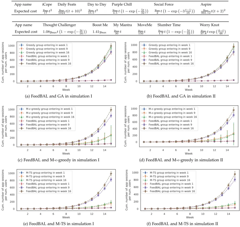
Fig. 3: Cumulative number of app sessions per number of users of groups 1, 3, and 9, for bandit-based algorithms in simulations I and II.
TABLE 3: The total number of app sessions of the last user group of the mini-simulation by end the last week, with the given scaling factor.
Scaling factor (↵) 1 12 14 18 161 321
Terminal reward 200 324 632 785 815 751 of last user group
6.3 Algorithms Used
We compare FeedBAL with both bandit-based and collab-orative filtering-based algorithms. The bandit algorithms
TABLE 4: The dropout rate of each algorithm in simulation II.
Algorithm Dropout rate (%) Standard deviation
Benchmark 4.16 0.135 FeedBAL 16.6 0.845 GA 16.6 0.930 M-✏n-greedy 28.7 8.21 M-TS 28.0 4.06 KNN 22.2 2.10 SVD 26.3 3.83
IEEE TRANSACTIONS ON SERVICES COMPUTING 10
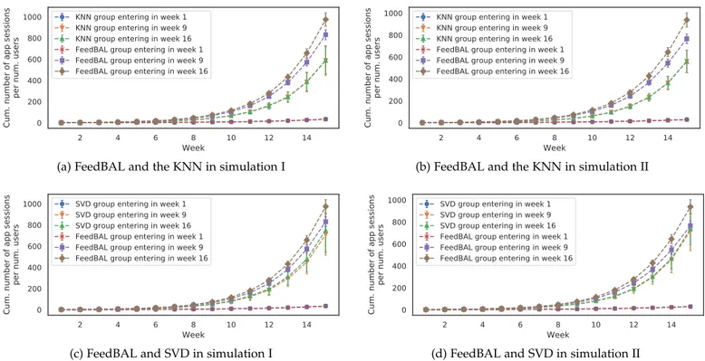
(a) FeedBAL and the KNN in simulation I (b) FeedBAL and the KNN in simulation II
(c) FeedBAL and SVD in simulation I (d) FeedBAL and SVD in simulation II
Fig. 4: Cumulative number of app sessions per number of users of groups 1, 3, and 9, for CF-based algorithms in simulations I and II.
Fig. 5: The colors representing each app. The apps are numbered in the following order: Aspire, Boost Me, Daily Feats, iCope, My Mantra, Day to Day, MoveMe, Purple Chill, Slumber Time, Social Force, Thought Challenger, and Worry Knot. include variations of Thompson Sampling and ✏n-greedy,
while the collaborative filtering algorithms are a neigh-borhood model based on K-nearest neighbors (KNN with baseline), and a factorization model based on singular value decomposition (SVD). Since our data only includes past interactions of users and apps, context-based approaches such as [11], [12], [13] are not suitable for our model. We would also like to note that collaborative filtering has been extended to use more complex techniques such as neural networks [39], however these models would not be suitable for our online setup due to the success of such models stemming from being trained on hundreds of thousands of training data.
FeedBAL: FeedBAL is used with the states, feedbacks,
costs, and actions defined in the previous subsection. Note that apps are continuously recommended and the stop action is only taken when it is the 16th week for the user, at which point the episode (user) is ended. Following the end of an episode, the learner observes the total number of app sessions during those 16 weeks as the terminal reward. The learner does not stop until the end because it makes more sense to collect the terminal reward at the end of 16 weeks, when it is maximum. Therefore, app recommendations are made in the first 15 weeks while the stop action is taken in week 16 and terminal reward is collected. Lastly, since the total number of app sessions can reach up to 2000 for
most users, FeedBAL needs at least 2000 ⇥ 15 = 30000 feedback/cost averages to keep track of. This not only drastically increases regret, but it also causes FeedBAL to use a lot of space. To address this issue, we discretize the states as follows: let the discretized version of x be denoted by xd. Then, xd :=
(
x, x 100,
bx
50c + 99, otherwise.
Note that this discretization does not change the states of the users, instead it changes the states seen by FeedBAL.
FeedBAL presented in Section 4 assumes that the sub-Gaussian parameter of the reward and cost distribution, , is known. However, as this may not be true when performing online recommendations, we make a small modification to FeedBAL so that it learns the parameter during the simu-lation. To do this, we assume that the reward distribution is -sub-Gaussian with standard deviation , meaning that to estimate , FeedBAL needs to keep track of the rewards it received and compute the sample standard deviation. Note that although the rewards in our simulations, which correspond to number of app sessions coming from the IntelliCare suite, follow a Poisson distribution, which is not sub-Gaussian, FeedBAL can still learn and recommend apps successfully because a Poisson distribution with mean can be approximated by a Gaussian with mean and variance , especially for large (see Theorem I of [40]). Lastly, even
(a) User group 1 of benchmark (b) User group 1 of all learning algorithms
(c) User group 16 of FeedBAL (d) User group 16 of GA
(e) User group 16 of M-✏-greedy (f) User group 16 of M-TS
(g) User group 16 of KNN (h) User group 16 of SVD
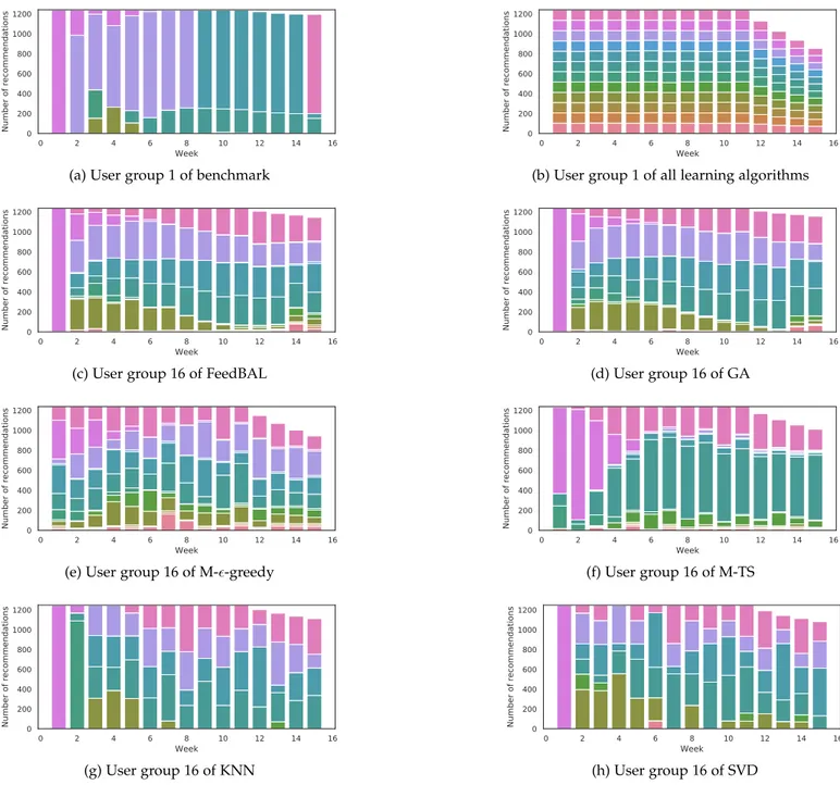
Fig. 6: The number of times each app was recommended in each week of simulation II for the first and last user groups of the benchmark, bandit algorithms and CF-based algorithms.
t=1 t=1 t=1 t=1 t=1 t=1t=1t=1t=1t=1t=1 t=2t=2t=2t=2t=2t=2 t=14t=14t=14t=14t=14t=14t=14t=15 t=16t=15t=15t=15t=15t=15t=15t=16t=16t=16t=16t=16t=16 t=15t=15t=15t=15t=15 t=16t=15 t=16t=15t=16t=16t=16t=16 1 2 16 17 Week (t) 1 2 16 17 Week (t)
Fig. 7: Batch user arrivals without user dropout. Note that t that is used for each user group is relative to when they entered the experiment. Also, observe that each user group stays for 16 weeks. For instance, the red users, who entered in week 1, leave at the end of week 16.
though the mean (and so standard deviation) of the rewards is a function of (t, x, a), we chose to only keep track of a
different for each t.
Since the cardinality of [lmax] ⇥ X ⇥ A is large, the
number of observations of each triplet (t, x, a) is small. In order to avoid having too many explorations, we multiply the confidence term by a scaling factor. In other words, u⇢t,x⇢ t,a := ˆg ⇢ t,x⇢t,a+ ↵· conf ⇢ t,x⇢t,a, where 0 < ↵ 1 in our simulations.
GA: GA stores the feedback and cost of recommending app
a in week t in (discretized) state x, and recommends the app with the highest sample mean feedback minus cost. In other words, GA is just like the FeedBAL algorithm with its confidence term (conf⇢
t,x⇢t,a) set to zero.
M-✏n-greedy and M-TS: Typical MAB algorithms like ✏n
-greedy [34] or TS [35] cannot directly be used in our setting, as the set of all sequences of app recommendations has
IEEE TRANSACTIONS ON SERVICES COMPUTING 12
cardinality 1215
⇡ 1.5⇥1016. If each sequence is regarded as
an arm, then these algorithms would always be exploring. Therefore, We use modified versions of ✏n-greedy and TS,
called M-✏n-greedy and M-TS, respectively, that make sense
in the context of our episodic app recommendation problem. In these two algorithms, 15 instances10 of ✏
n-greedy (with
c = 0.8 and d = 0.1) and 15 instances of TS11 are used,
respectively, with one assigned to each week. For example, to recommend an app in week t using M-TS, the respective M-TS instance for that week will be used and once the feedback and cost arrive, only that TS agent’s mean reward will be updated.
KNN with baseline: KNN with baseline, or KNN for short,
is a neighborhood model that uses an item-based approach that predicts a user’s rating for an app based on other apps that the user has rated. Rating prediction is made using the closest 40 user-item pairs and with a weighted sum with a baseline. We refer readers to Section 2.2 and more specifi-cally Equation 3 of [41] for the details of how the rating is generated. The closest 40 pairs are determined using Pear-son’s correlation coefficient as the similarity measure. We use the Python library Surprise12 and more specifically its
KNNBaseline class for the implementation of this algorithm.
Matrix factorization with SVD: In matrix
factorization-based approaches, the user-app-rating matrix is broken down into a product of smaller matrices, in this case using SVD. The basic idea is that the broken down matrices can provide implicit and hidden information about user-app interactions that are otherwise unused when directly using the user-app-rating matrix. We use the matrix factorization based algorithm of [41], described in Section 3 and Equation 5. We also use the Surprise library for this algorithm’s implementation; more specifically the SVD class.
For both CF-based algorithms, we use feedback minus cost, scaled to [0, 1], as the rating. The user-app-rating ma-trix is filled throughout the experiment and training/data-fitting using the matrix is done at the end of each week. Moreover, when a new user arrives who has no recorded app interactions, he is recommended an app at random.
6.4 Results
For the simulations, we set lmax= 16and = 0.01 in
Feed-BAL. Furthermore, all simulations were ran and averaged on five different user arrival samples, with each simulation being repeated eight times per sample for a total of 40 runs. For FeedBAL, we first ran mini-simulations on 2000 users without dropouts with ↵ 2 {1,1
2, 1 4, 1 8, 1 16, 1 32} and recorded
the total number of app sessions of the last user group by end the last week (i.e, terminal reward of last user group); this data can be seen in Table 3. We then picked the ↵ corresponding to the highest terminal reward, which was
1
16, and performed simulations I and II.
10. We use 15 instances because the action taken in week 16 is always the stop action.
11. The update rule is as follows: reward, i.e., feedback minus cost, is observed and scaled to [0, 1]. Then, a Bernoulli distribution with probability equal to the scaled reward is sampled. Finally, the a/b
parameter is incremented by one if the sample is 1/0. The scaling factor is learned by each TS agent (i.e., when a new reward that is higher than the current scaling factor is observed, the scaling factor is set to that reward).
12. Link: http://surpriselib.com.
Fig. 3a-3f show the cumulative number of app sessions observed by three user groups entering in week 1, 9, and 16, up to and including week t, achieved by the bandit-based algorithms in simulations I and II, and Fig. 4a-4d show the same for CF-based algorithms. The x-axis is the relative week number of the user. For instance, if a user enters the experiment in the 13th week and has y app sessions, then ywill be added to app sessions of week 1 as he observed y sessions in his first week of entering the experiment.
When compared with other bandit algorithms, FeedBAL manages to outperform the other algorithms and achieve substantial improvement over M-✏n-greedy and M-TS as
the experiment proceeds (e.g. from week 9 to week 16) in both simulations. The GA performs the closest to FeedBAL, having done so as a result of the nature of the data, where the difference between the user app session counts of the top apps in each week is not small. Hence, in other settings where the difference between the reward of the optimal action and the reward of the next optimal action is small, we expect the difference between GA and FeedBAL’s per-formance to grow.
FeedBAL also manages to outperform CF-based algo-rithms. Notice that both KNN and SVD do not provide any major improvement from week 9 to week 16, which indicates that they have maximized the information coming solely from user-app interactions at the end of week 9. In other words, FeedBAL outperforms them because it takes into account in which week and with how many previous app sessions (state) a user was given an app recommenda-tion when making decisions for future users. On the other hand, both KNN and SVD do not take into account week or state.
When it comes to simulation II, M-✏n-greedy and M-TS
also perform poorly as they cannot learn how to recommend the best apps fast enough, which results in a significant drop in the cumulative number of app sessions. This stems from their failure to exploit the state information. KNN and SVD perform slightly better with user dropouts and SVD even gets very close to FeedBAL, as seen in Fig. 4d, but FeedBAL still manages to outperform them all.
To demonstrate that the actions taken by FeedBAL ap-proach those taken by the benchmark that picks apps with the highest expected feedback, we look at the number of times each of the twelve apps were recommended by the benchmark and all four algorithms during simulation II. We expect that FeedBAL will recommend apps randomly (ex-ploration) for the first user group, while it will recommend the apps it has learned to give the highest reward minus cost (exploitation) for the last user group. Our expectations were accurate and the results can be seen in Fig. 6a to 6h. These figures show the number of times each app was recommended in each week using stacked bar charts, where each color represents an app. Fig. 5 shows the app to color mapping. Notice that all learning algorithms recommend all apps the same number of times for the first user group (Fig. 6b), with the reason being that when recommending apps to the users in the first user group, each bandit algorithm is seeing each week for the first time and each CF-based algorithm is seeing the users for the first time and so they recommend apps randomly. Furthermore, the benchmark recommends the same apps for each user group, hence the
illustration of apps recommended for user group 1 (Fig. 6a) is representative of all user groups.
While all bandit algorithms learn something by the time the last user group enters the experiment, only GA and FeedBAL manage to learn the correct apps (i.e., those with the highest feedback minus cost mean, which are picked by the benchmark). Visually, notice that not only did the the number of colors, each of which represents an app, decreased from user group one to user group sixteen of FeedBAL (Fig. 6b to Fig. 6c), but so did the drop in col-umn heights. These two visual changes, which represent the learning of app rewards/costs and decrease in user dropouts, respectively, are hardly present in the figures of M-✏n-greedy and M-TS.
The CF-based algorithms did fare better than the bandit ones (excluding GA and FeedBAL), but their downfalls are not using week/state information and their lack of exploration. Visually, notice that only a few apps are rec-ommended by KNN and SVD (few distinct colors in Fig. 6g and 6h), while FeedBAL recommends nearly every app in most weeks (many distinct colors in Fig. 6c).
We present the dropout rates of each algorithm, defined as the number of users that dropped out divided by total number of users that entered the experiment, in Table 4. Observe that FeedBAL and GA achieve the lowest dropout rate, which is 12.1, 11.4, and 9.7 percent lower than those of M-✏n-greedy, M-TS, and SVD respectively. This result is
also visible in Fig. 6a to 6c, where FeedBAL and GA achieve the lowest drop in bar height after week 12 of the last user group. KNN performs the second best after FeedBAL and GA, but it is still significantly behind at 22.2 percent, versus the 16.6 percent dropout rate of FeedBAL and GA.
Lastly, the apps chosen by FeedBAL for the last user group resemble those chosen by the benchmark much more than M-✏n-greedy and M-TS, as evident by the similar colors
in Fig. 6c and 6a. KNN and SVD recommend similar apps when compared with FeedBAL, with the main difference being a lack of exploration, which as mentioned previously hinders their performance.
Note that although overall GA performs just under FeedBAL, it does not mean it will always do so in every simulation setting and on every dataset. Rather, it highlights the fact that the user data was skewed and users of Intelli-Care mostly used one or two of the twelve apps. Had the data have been better distributed with all apps equally used, then we would expect to see GA get stuck in recommending a suboptimal app.
7 C
ONCLUSIONWe proposed a new class of online learning methods for application recommendation. Although the number of pos-sible sequences of actions increases exponentially with the length of the episode, we proved that an efficient online learning algorithm that has expected regret that grows poly-nomially in the number of steps and states, and logarith-mically in the number of episodes exists. We also showed that the proposed algorithm outperforms ✏n-greedy and TS
based learning methods and CF based learning methods.
A
CKNOWLEDGMENTSThe authors would like to thank Ken Cheung and Xinyu Hu of Columbia University for providing us with IntelliCare data that was used in the simulations. The work of Cem Tekin was supported by BAGEP 2019 Award of the Science Academy.
R
EFERENCES[1] Z. Zheng, H. Ma, M. R. Lyu, and I. King, “QoS-aware web service recommendation by collaborative filtering,” IEEE Trans. Services Comput., vol. 4, no. 2, pp. 140–152, 2010.
[2] L. Song, C. Tekin, and M. van der Schaar, “Online learning in large-scale contextual recommender systems,” IEEE Trans. Services Comput., vol. 9, no. 3, pp. 433–445, 2014.
[3] R. Liu, J. Cao, K. Zhang, W. Gao, J. Liang, and L. Yang, “When privacy meets usability: unobtrusive privacy permission recom-mendation system for mobile apps based on crowdsourcing,” IEEE Trans. Services Comput., vol. 11, no. 5, pp. 864–878, 2016. [4] O. Khalid, M. U. S. Khan, S. U. Khan, and A. Y. Zomaya,
“Om-niSuggest: A ubiquitous cloud-based context-aware recommen-dation system for mobile social networks,” IEEE Trans. Services Comput., vol. 7, no. 3, pp. 401–414, 2013.
[5] B. Liu, Y. Wu, N. Z. Gong, J. Wu, H. Xiong, and M. Ester, “Struc-tural analysis of user choices for mobile app recommendation,” ACM Trans. Knowl. Discovery Data, vol. 11, no. 2, pp. 1–23, 2016. [6] M. Terry, “Medical apps for smartphones,” Telemedicine and
e-Health, vol. 16, no. 1, pp. 17–23, 2010.
[7] K. Hirsh-Pasek, J. M. Zosh, R. M. Golinkoff, J. H. Gray, M. B. Robb, and J. Kaufman, “Putting education in “educational” apps: Lessons from the science of learning,” Psychol. Sci. Public Interest, vol. 16, no. 1, pp. 3–34, 2015.
[8] D. C. Mohr, K. N. Tomasino, E. G. Lattie, H. L. Palac, M. J. Kwasny, K. Weingardt, C. J. Karr, S. M. Kaiser, R. C. Rossom, L. R. Bardsley et al., “Intellicare: an eclectic, skills-based app suite for the treatment of depression and anxiety,” J. Med. Internet Res., vol. 19, no. 1, p. e10, 2017.
[9] Y. K. Cheung, B. Chakraborty, and K. W. Davidson, “Sequential multiple assignment randomized trial (SMART) with adaptive randomization for quality improvement in depression treatment program,” Biometrics, vol. 71, no. 2, pp. 450–459, 2015.
[10] E. M. Luef, B. Ghebru, and L. Ilon, “Language proficiency and smartphone-aided second language learning: A look at english, german, swahili, hausa and zulu.” Electronic Journal of e-Learning, vol. 17, no. 1, pp. 25–37, 2019.
[11] H. Zhu, E. Chen, H. Xiong, K. Yu, H. Cao, and J. Tian, “Mining mobile user preferences for personalized context-aware recom-mendation,” ACM Trans. Intell. Syst. Technol., vol. 5, no. 4, pp. 1–27, 2014.
[12] T. Liang, L. Zheng, L. Chen, Y. Wan, S. Y. Philip, and J. Wu, “Multi-view factorization machines for mobile app recommenda-tion based on hierarchical attenrecommenda-tion,” Knowledge-Based Systems, vol. 187, p. 104821, 2020.
[13] C. Liu, J. Cao, and S. Feng, “Leveraging kernel-incorporated matrix factorization for app recommendation,” ACM Trans. Knowl. Discovery Data, vol. 13, no. 3, pp. 1–27, 2019.
[14] S. A. Murphy, “Optimal dynamic treatment regimes,” J. R. Stat. Soc.: Series B (Stat. Methodol.), vol. 65, no. 2, pp. 331–355, 2003. [15] J. M. Robins, “Optimal structural nested models for optimal
se-quential decisions,” in Proc. 2nd Seattle Symposium in Biostatistics, 2004, pp. 189–326.
[16] S. A. Murphy, “An experimental design for the development of adaptive treatment strategies,” Statistics in Medicine, vol. 24, no. 10, pp. 1455–1481, 2005.
[17] D. Blatt, S. A. Murphy, and J. Zhu, “A-learning for approximate planning,” Ann Arbor, vol. 1001, pp. 48 109–2122, 2004.
[18] P. J. Schulte, A. A. Tsiatis, E. B. Laber, and M. Davidian, “Q-and A-learning methods for estimating optimal dynamic treatment regimes,” Stat. Sci., vol. 29, no. 4, p. 640, 2014.
[19] Y. Gai, B. Krishnamachari, and R. Jain, “Combinatorial network optimization with unknown variables: Multi-armed bandits with linear rewards and individual observations,” IEEE/ACM Trans. Netw., vol. 20, no. 5, pp. 1466–1478, 2012.
[20] N. Cesa-Bianchi and G. Lugosi, “Combinatorial bandits,” J. Com-put. Syst. Sci., vol. 78, no. 5, pp. 1404–1422, 2012.