Map building with multiple range measurements using morphological surface profile extraction

(1)

Map Building with Multiple Range Measurements

Using Morphological. Surface Profile Extraction

Billur Barshan

Deniz Bagkent

Department

of

Electrical Engineering

Bilkent University

Bilkent, 06533 Ankara, Turkey

billur@ee.

bilkent

.edu.tr

Department

of

Biomedical Engineering

University

of

Southern California

Los

Angeles, CA 90089-1451

U.S.A.

baskent Qscf

.use.

edu

Abstract

A novel method is described for surface profile ex-

traction based on morphological processing of multiple range sensor data. The approach taken is extremely flexible and robust, in addition to being simple and straightforward. It can deal with arbitrary numbers and configurations of range sensors as well as syn- thetic arrays. The method has the intrinsic abality

t o suppress spurious readings, crosstalk, and higher- order reflections, and process multiple reflections in- formatively. The essential i d e a of this work-the use of multiple range sensors combined with morphological processing-can be applied to different physical modal-

ities of range sensing of vastly different scales and in many diflerent areas. These may include radar, sonar, robotics, optical sensing and metrology, remote sens- ing, ocean surface exploration, geophysical exploration, and acoustic microscopy.

1.

Introduction

An inexpensive, yet effective and reliable approach to machine perception is to employ multiple simple range sensors coupled with appropriate data processing. This paper deals with the determination of azbi- trary surface profiles, and is completely novel in ],hat morphological processing is applied to range data in the form of an arc map, representing angular uncertainties. The method is extremely flexible and can easily handle arbitrary sensor configurations, as well as synthetic arrays. In contrast, approaches based on geometrical or analytical modeling are often limited to elementary target types or simple sensor configurations [I, f', 51.

A commonly noted disadvantage of range sensors if, the

difficulty associated with interpreting spurious read-

ings, crosstalk, higher-order, and multiple reflections. The proposed method is capable of eiffectively suppress- ing the first three of these, and informatively processing echoes returning from surface feakures further away than the nearest (i.e. multiple reflections).

surface 't surface

sensitivity region sensitivitv renion ~I

transmittingheceiving transniitting receiving sensor sensor sensor

(a) (b)

Figure 1. Transmitter and receiver are (a) 'the

same device, (b) separate deviices.

Despite the generality of the method, for concrete- ness, we consider simple range sensors that measure time-of-flight (TOF) t o , which is thLe round-trip travel time of the pulse between the sensor and the object. Given the speed of transmission c, the range r can be

easily calculated from T = c t 0 / 2 . Although such devices return accurate range data, typically the;y cannot provide direct information on t he angular position of the object from which the reflection was obt,ained.

Thus, all that i s known is that the reflection point lies on a circular arc of radius r (Fig. l (a)). More gener- ally, when one sensor transmits and another receives, it is known that the reflection point lies on the arc O F

an ellipse whose focal points are the transmitting ancl receiving elements (Fig. l( b)). The arcs are tangential to the surface at the actual point(s) of reflection.

Most commonly, the wide beamwidth of the sensoi: is accepted as a device limitation that determines the

(2)

angular resolving power of the system, and the reflection point is assumed t o be along the line-of-sight. In our method, circular or elliptical arcs, representing the uncertainty of the object location, are drawn. By com- bining the information inherent in a large number of such arcs, angular resolution far better than that im- plied by the beamwidth is obtained.

2.

Morphological

profile

extraction

500

i::m

-

A200 100 ~

.'

.

0 100 200 300 400 500 x (pixels)

(4

5 0 0 7 1 500 400 5300 .g P

-

_woo l o o t

-

<.

I '

1 . .

0 100 200 300 400 500 x (pixels) (b)

Structured sensor configurations such as linear and circular arrays as well as irregularly configured sensors have been considered in [3], where the method is also generalized to moving sensors and synthetic arrays.

To illustrate the method, Fig. 2(a) shows a surface whose profile is to be determined by using an irregular sensor configuration. A large number of arcs can be obtained with a reasonably small number of sensors because each sensor can receive pulses transmitted from all the others, provided a reflection point lies in the joint sensitivity region for that sensor pair. Fig. 2(b) shows the arcs obtained. Although each arc represents considerable uncertainty as to the angular position of the reflection point, nevertheless one can almost extract the actual curve shown in Fig. 2(a) by visually examining the arc map in Fig. 2(b). Each arc drawn is expected to be tangential to the surface at least at one point. At these actual reflection point(s), several arcs will intersect with small angles at nearby points on the surface. The many small segments of the arcs superimposed in this manner coincide with and cover the actual surface, creating the darker features in Fig. 2(b) that reveal the surface profile. The remaining parts of the arcs, not actually corresponding to any reflections and simply representing the angular uncertainty of the sen-

sors, remain more sparse and isolated. Similarly, those arcs caused by higher-order reflections, crosstalk, and noise also remain sparse and lack much reinforcement. In this study, morphological operators are used to eliminate the sparse and isolated segments in the arc map, leaving behind the mutually reinforcing segments that reveal the solid structure of the original surface. Erosion, dilation, opening, closing, and thinning are widely used morphological operations to accomplish tasks such as edge detection, skeletonization, segmen- tation, texture analysis, enhancement, and noise re- moval in image processing [4]. Most applications involve processing of conventional binary or gray-scale images, or range images where the range information is coded in the gray-levels of the image [7]. The present approach is completely novel in that morphological processing is applied to range measurements in the form of an arc map, representing angular uncertainties.

0 100 200 300 400 500 x (pixels) (c) 0 100 200 300 400 5W x (pixels) (d)

Figure 2. (a) The actual surface and the sen-

sors, (b) the arc map obtained with 17 sen-

sors, each of 45O beamwidth, (c) the result of

n

=

6 thinning, (d) the fitted curve (solid line) and the original surface (dashed line).

Morphological operations basically consist of a set of simple rules t o modify images. A simple algorithm

for erosion is as follows: If all eight neighbors of a pixel

with value one equal one, that pixel preserves its value, otherwise its value is set equal to zero. This way, the image will be eroded or shrunk in all directions by one pixel. On the other hand, dilation is used to fatten an image: all eight neighbors of those image pixels which originally equal one are set equal to one.

Thinning is a generalization of erosion with a pa-

rameter n varying in the range l

<

n

<

8. In this case, it is sufficient for any n neighbors of a pixel to equal one in order for that pixel to preserve its value of one. The flexibility that comes with this parameter enables one to make more efficient use of the information con- tained in the arc map. Thus, pruning and erosaon are the two extremes of thinning with n = 1 and n = 8.

The result of applying n = 6 thinning to the arc map shown in Fig. 2(b) is presented in Fig. 2(c). As a last step, a least-squares polynomial fit is obtained to compactly represent the surface profile. The curve fitted to the thinned map in Fig. 2(c) is displayed in Fig. 2(d). A a root-mean-square absolute error measure E =

J&

C~,l[P(z~) - y(zi>]2 is introduced, com- paring the final polynomial fit with the actual curve. Here N is the total number of columns in the map ma- trix, p ( ~ ) are the samples of the fitted polynomial, and

(3)

the actual surface profile y(x:;). The result of applying various morphological operators t o the arc map in Fig. 2(b) are summarized in Table 1.

1

morphological operation

I

$(pixels)

1 tCp,(s:d

thinning (n = 1 : pruning) thinning ( n = 3) thinning ( n = 6) 2.75 0.98 thinning ( n = 7) 5.29 0.97 thinning ( n = 5) 0.99 - \ 11.50 5.64 11.75 thinning ( n = 8 : erosion) closing & erosion

Table 1. Results of various morphological op-

erations.

A detailed study of the performance of different sensor configurations and morphological operations has been performed. Structured arrays are often preferred in theoretical work for simplicity and ease of analysis, whereas the method presented here can handle irregular arrays equally easily. Although the problein of optimal sensor placement is a subject for future research, the large number of simulations performed in- dicate that it is preferable to work with irregular arrays, since the randomized vantage points of the sensors tend to complement each other better than structured ones. In a typical robotics application, these sensors may constitute an array on the same robot, or may correspond to sensors onboard different robots explor- ing the environment.

I

E (pixels)

I

t,,,

<a

I

thinnine: ( n = - \ 1 : Druning) V I

I

4.98

I

1.9

r - 7

thinning ( n = 2) 4.84 thinning ( n = 3)

_-~

4.07 thinning ( n = 4) 3.28 thinning ( n = 5) 2.58 thinning ( n = 6) 1.96 thinning ( n = 7) thinning (n = 8 : erosion) erosion & pruning (n = 1)

1.93

Table 2. Experimental results for the surface

in Fig. 3(a).

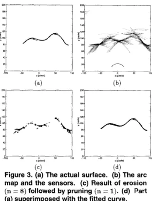
The method has been tested with real sonar data, experimentally obtained from a Nomad 200 mobile robot, initially using smooth cardboard surfaces. An example is shown in Fig. 3 for which additional results are provided in Table 2. Even though the method

-lw -M 0 Y) 1w -100 -M 0 yi I W

x l 9 l X ~ I S l x (psslal

( c )

(4

Figure 3. (a) The actual surface. (b) The arc

map and the sensors. (c) Result of erosion

(n = 8) followed by pruning (:n = 1). (d) IPart (a) superimposed with the fitted curve.

was initially developed and demclnstrated for specu- larly reflecting surfaces, subsequent, tests with Lamber- tian surfaces of varying roughness have indicated that the method also works for rough surfaces, with errors slightly increasing with roughness.

3.

Performance

of

the method

Although the method is applica,ble to arbitrary sur-

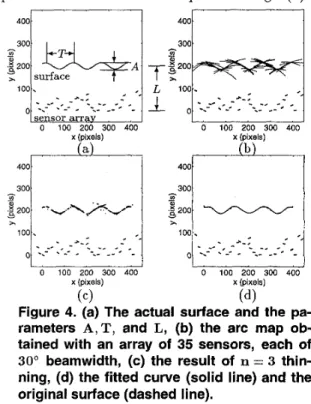
faces [3], to investigate the performance of the method, sinusoidal surfaces have been considered whose parameters can be systematically varied. Simulations have been undertaken on sinusoidal surfaces of varying amplitude and periodicity, located at varying distances from the sensor array. These pararneters are illustrated in Fig. 4(a). The elements of the sensor array are di;+ tributed in the box [-35,4401 x

[O,

901, with t;heir av- erage distance from y = 0 being 32.7 pixels.

We investigate the dependence of the error on a m p l i tude, period, surface distance, sensor beamwidth, and measurement uncertainty. For this purpose, the sinusoid shown in Fig. 4(a), with A = 30, T = 125, arid

L = 200 pixels, is taken as a reference and these parameters are individually varied around the reference values. The arc map generated is shown in part (b) of the same figure. The result of n = 3 thinning, which gives the minimum error for this example, is given in

(4)

part (c). The resulting error when various morphological operators are applied to the same arc map are summarized in Table 3. Finally, the result of curve fitting, and the comparison with the actual surface are given in part (d).

First, the period is varied by keeping the amplitude and the surface distance constant at the reference values given above. € increases with decreasing period as expected (Fig. 5(a)). For periods shorter than 100 pixels, the error increases significantly. The minimum radius of curvature Rmin is a useful indicator of the difficulty of extracting the profile: features with smaller radii of curvature are more difficult t o accurately determine. For this reason, the relation between Rmin and the period of the sinusoid is also plotted in Fig. 5(b).

In the next step, the amplitude is varied while keeping the period and the distance constant at the reference values. € increases with increasing amplitude (Fig. 5(c)), since increasing A reduces Rmin. Rmin is plotted as a function of the amplitude in Fig. 5(d).

400/1 1-1004 300 300

. -. -

. ~-

- 0 100 200 300 400 0 100 200 300 400 x bixels) x (Dixels) _.. _. I ' (a) I , (b) 1

400t

300 400

1

1001 ,

.,

->-:

:;I

I O I t - ,

_-

.,

-*-:

-

-I ,

-

:;*I

-.-

.

--

- -.-

__

e

-

- _-

. - _ -

~ 0

..-

.

--

- -.-

_-

'

-

0 100 200 300 400 0 100 200 300 400 x (pixels) x (pixels) (c) ( 4

Figure 4. (a) The actual surface and the pa-

rameters A , T , and L, (b) the arc map ob-

tained with an array of 35 sensors, each of

30' beamwidth, (c) the result of n = 3 thin- ning, (d) the fitted curve (solid line) and the original surface (dashed line).

To get a better understanding of the relation between the error and curvature, the results in Fig. 5 are rearranged to generate a plot of € versus Rmin (Fig. 6).

As expected, decreasing the curvature (or increasing Rmin) results in lower E . The fact that the solid and dashed lines (which represent varying T and A respec-

tively) follow each other closely, suggests that what really matters is not the individual values of T and A, but the value of Rmin.

I

€(pixels)

I

thinning ( n = 1 : pruning)

I

2.41

I

thinning ( n = 2)

thinning ( n = 3)

thinning ( n = 4) 2.09

thinning ( n = 5) 2.46

I closine: & Drunina ( n = 11

I

2.61 I closing & thinning ( n = 3)

I

3.02 closing & erosion ( n = 8)

I

3.63

Table 3. Results of various morphological op- erations.

Ok

125 175 225 52; T (pixels) W 10 10 20 30 40 50 A (pixels) A (pixels) ( c )

(4

Figure5 (a)E VS. T, (b) R m i n VS. T, (c)Evs. A,

(d) R,,, vs. A.

Figure 6. E vs. R m i n . Solid dots connected by solid lines are produced by eliminating T from Fig. 5(a) and (b). Triangles connected by

dashed lines are produced by eliminating A

(5)

40i----

4

0 r

1

beamwidth 5O

c *

- .

L O 150 260 250 3C!O ‘0 ₃₀ ₆₀ ₉₀

L (pixels) beamwidth (deg)

none 3.411

(a) (b)

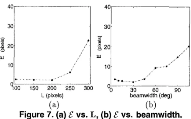
Figure 7. (a) E vs. L, (b) E vs. beamwidth.

Next, the distance to the surface is varied while A

and T are kept constant at their reference values. E increases as L increases beyond 250 pixels (Fig. 7(a)). Because the surface shape does not change, the curvature remains constant. Details about the processing involved to generate Fig. 7(a) are presented in Table 4. Since the number of arc points obtained strongly depends on L , and the most suitable morphological operation depends strongly on the density of arc points, the morphological procedure best suited to each value of L has been employed in constructing

Fig. 7(a). (In addition to the alternatives shown in Ta- ble 3, n = 6 , 7 , 8 thinning, and the application cif no morphological processing at all have been conside red.) For a given beamwidth, when the surface is located further, the arcs become larger and uncertainty in the position of the reflection point(s) increases. In a way, the “effective” curvature of the surface increases with increasing L , resulting in larger errors. Geometrically, this is the same effect as perceiving a curved object to be flatter when we are very close to it, and more curved when further away. A distinct issue arises when the dis-

tances are very small: the arcs become very short in length and less in number, since now sensors can de- tect a smaller portion of the surface and there is less overlap between their sensitivity patterns. As a result, the arc map cannot cover the whole surface.

Another important parameter is the sensor beamwidth. To investigate the effect of the sensor beamwidth, the surface parameters are kept constant while the beamwidth is varied. Increasing the beamwidth results in arcs longer in length, causing a larger portion of each arc to be redundant. In other words, there is more uncertainty in the position of the reflection point(s) as compared to the case of a

narrower beamwidth. As a result, the error increases as shown in Fig. 7(b). The arcs also increase in number, and these factors make it necessary to apply higher-n thinning to extract the useful information. On the other hand, when the beamwidth is very small, the arcs become very short and fewer in number,

(pixels) operation (pixels)

I

100

I

thinning ( n = 1‘)

I

2.43

I

2.03 200 thinning ( n = 3 )

thinning ( n = 4) 22.71

Table 4. Results corresponding to Fig. 7(a).

thinning ( n = 3) 2.03

t

105” thinning in

=--I

Table 5. Results corresponding to Fig. 7gb).

leading to a similar situation as when L was very small. Below a beamwidth of 15O, directly fitting a polynomial to whatever few points are available in the arc map, without applying morphological processing, becomes the best choice. This customization of the applied morphological rule enables a fair com parison of the results at all beamwidth values. Smaller beamwidths result in fewer arc points and thus l e s reliable curve fits, leading to a slight increase in the error for very small beamwidths. Best results are obtained for a particular beamwidth (about 30’ in our example). The different morphological operations applied and the resulting error values are tabulated in Table 5. Choosing beamwidths smaller than 30’ does not increase the error appreciably, however using sensors with smaller beamwidths rnay not be desirable anyhow, since these are usually more diffil:ult to manufacture, expensive, or enta.il a trade-off with some other quantity. For instance, in the case of

acoustic sensors, narrower beamwidth devices must have higher operating frequencies, which imply greater attenuation in air and shorter operating range.

Now, we discuss the issue of choice of sampling r e - olution or pixel size: There are a couple of factors that determine the accuracy of T O F readings in a rang;e measurement system. One of these factors is the operating wavelength of the ranging s,ystem: a TOF mea-

(6)

4 0

- 4.

Conclusions

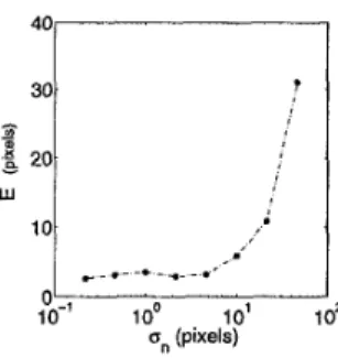
Figure 8. 8 vs. noise standard deviation.

surement with accuracy better than the wavelength cannot be normally achieved. Other sources of uncertainty in the range measurement could be effects such as the thermal noise in the receiving circuitry or the ambient noise. Given these, it is not meaningful to choose the pixel size much smaller than the resolving limit determined by these factors, since it would increase the computational burden without resulting in a more accurate profile determination. Thus, the pixel size should be chosen comparable to the T O F measurement accuracy. Nevertheless, since the T O F accuracy may not be known beforehand, we have examined the cases where the noise or uncertainty is both smaller and larger than one pixel.

To investigate the robustness of the method to noise, zero-mean white Gaussian noise has been added to the TOF readings. The noise standard deviation 6, is var-

ied logarithmically to cover a broad range of noise levels. As expected, for C T ~ smaller than one pixel, the per-

formance is approximately the same as for the noiseless case. This performance can be further improved by re- ducing the pixel size until it becomes comparable to the TOF measurement accuracy, at the cost of greater computation time.

The error increases significantly as the noise level increases beyond one pixel (Fig. 8). Since the method relies on the mutual reinforcement of several arcs to reveal the surface, larger amounts of noise are expected to have a destructive effect on this process by moving the various arc segments out of their reinforcing positions. Consequently, the arc segments which now lack each other’s mutual reinforcement tend to be eliminated by the morphological operations. A larger proportion of the arcs is eliminated, resulting in a loss of information characterizing the original curve. Nevertheless, the error growth rate is not as high as might be suggested by these arguments, and the method seems to be reasonably robust to measurement uncertainty. In Fig. 8, the performance is comparable to the noiseless case up to

U , = 10 pixels. This is partly because the least-squares

polynomial fit helps eliminate some of the noise.

A novel method is described for determining arbitrary surface profiles by applying morphological processing t o data acquired by simple range sensors. The method is extremely flexible, versatile, and robust, as well as being simple and straightforward. It can deal with arbitrary numbers and configurations of sensors, including synthetic arrays. Accuracy improves with the number of sensors used and can be as low as a few pixels except when the radius of the curvature is very small. The method is robust in many aspects: it has the inherent ability to eliminate undesired T O F readings arising from higher-order reflections, crosstalk, and noise, as well as processing multiple echoes informatively.

The CPU times for the morphological operations (when implemented in the C programming language and run on a 200 MHz Pentium Pro PC) are gener- ally about a quarter of a second [3], indicating that the method is viable for real-time applications. The method can be readily generalized t o 3-D environments with the arcs replaced by spherical or elliptical caps and the morphological rules extended to 3-D [6]. In certain problems, it may be preferable t o reformulate the method in polar or spherical coordinates. Some applications may involve an inhomogeneous and/or anisotropic medium of propagation. I t is envisioned that the method could be generalized in such cases by constructing broken or non-ellipsoidal arcs.

References

B. Barshan and R. Kuc. Differentiating sonar reflections from corners and planes by employing an intel- ligent sensor. I E E E Trans. o n Pattern Analysis and Machine InteZZigence, 12(6):560-569, June 1990. C. S. Chen, Y. P. Hung, and J. L. Wu. Extraction of corner-edge-surface structure from range images using mathematical morphology. I E I C E Trans. o n Informa- tion and Systems, E78D(12):1636-1641, 1995.

D. Bagkent and B. Barshan. Surface profile determination from multiple sonar data using morphological processing. Int. J. of Robotics Research, to appear in 2000.

E. R. Dougherty. An Introduction to Morphological Image Processing. SPIE Optical Engineering Press,

Bellingham, WA, U . S . A . , 1992.

L. Kleeman and R. Kuc. Mobile robot sonar for target localization and classification. Int. J. of Robotics Research, 14(4):295-318, August 1995.

K. Preston. 3-dimensional mathematical morphology. Image and Vision Computing, 9(5):285-295, 1991. J. G. Verly and R. L. Delanoy. Some principles and applications of adaptive mathematical morphology for range imagery. Opt. Eng., 32(12):3295-3306, 1993.