Nonlinear observer design with application to the synchronization of chaotic systems

: ■; | § | 1 | | f | | W íñ ». '»5^. U_{:f; г: :.' ·.." ·} Ч ;’!^. '■' *'■?.' ’· /, іГ · ν· >. _{^.1 Ц Ц. ■ t ІЦ I. ■}s·; ·7» . V, . · ·· ν -_{■ г’ · '} ^ “I Í’· Ѵ'·^ .f¿· ■ ■' '■% ΐΚίϊ'' W-ЧІ i» у . >·/ . « !..^< ñ T- 'fí *. í?V·· -s»’*/ Ş “И· 4it ■ >ί···^·..Λ//·;.··· T^·’ ií ^ V л с т я г о л і. 'm D ' ·""·-- λ*\ζ\'2·'j !Ρ,-ίΞW¿ ''3 < Í A β τ ν

SéS

NONLINEAR OBSERVER DESIGN WITH

APPLICATION TO THE SYNCHRONIZATION OF

CHAOTIC SYSTEMS

A THESIS

SUBMITTED TO THE DEPARTMENT OF ELECTRICAL AND

ELECTRONICS ENGINEERING

AND THE INSTITUTE OF ENGINEERING AND SCIENCES

OF BILKENT UNIVERSITY

IN PARTIAL FULFILLMENT OF THE REQUIREMENTS

FOR THE DEGREE OF

MASTER OF SCIENCE

By

Ercan Solak August 1996

Gl(\ • S 6 5 і з а б о f I ·{," f ’ 'S

I certify that I have recicl this thesis and that in my opinion it is fully ci' in scope ¿md in quality, as a thesis lor the degree of Master of Science.

U m i

----^

---A sso^Prof. Dr. Omfer Morgul(Supervi.sor)

te.

I certify that I have read this thesis and that in my opinion it is fully adequcite, in scope and in quality, as a thesis for the degree of Master of Science.

Prof. Dr. Erol Sezer

I certify that I have read this thesis and tluit in my opinion it is fully cidequate, in scope and in quality, as a thesis for the degree of Master of Science.

Prof. Dr. Bülent Özgüler

Approved for the Institute of Engineering and Sciences:

Prof. Dr. Mehmet fe ra y

Director of Institute of Engineering and Sciences

ABSTRACT

NONLINEAR OBSERVER DESIGN WITH APPLICATION

TO THE SYNCHRONIZATION OF CHAOTIC SYSTEMS

Ercan Solak

M.S. in Electrical and Electronics Engineering

Supervisor: Assoc. Prof. Dr. Omer Morgiil

August 1996

Observers cire used to estimate the states of dynamiccil systems whenever are not available through direct measurements. Although the design of lin­ ear observers is a well-developed branch of control theory, its counterpart for nonlinear systems is a relatively new field.

In this thesis, an observer construction methodology is proposed lor a chiss of nonlinear systems satisfying certain conditions. Then, the problem of syn­ chronizing chaotic systems, which has found recent appliccitions in the area of secure message transmission, is addressed from the observer design point of view. In the design, we exploited one of the essential properties of the chaotic systems that the trajectories remain in a bounded region of the state space. It is also shown that, for certciin well-known chaotic systems, the system structure enables one to nse linecir observer schemes in order to have global synchroniza­ tion.

Keywords : Nonlinear observers, chaotic systems, cluios synchronization.

ÖZET

DOĞRUSAL OLMAYAN GOZLEYICI TASARIMI VE

KAOTİK SİSTEMLERİN EŞZAMANLAMASINA

UYGULANMASI

Ercan Solak

Elektrik ve Elektronik Mühendisliği Bölümü Yüksek Lisans

Tez Yöneticisi: Doç. Dr. Ömer Morgül

Ağustos 1996

Gözleyiciler, dinamik sistemlerin durumları doğrudan ölçümlerle elde edilemediğinde, bu durumları tahmin etmekte kullanılırlar. Idoğrusal gözleyici tasarımı, kontrol kuramının gelişmiş bir dalı olmasına rağmen, bunun doğrusal olmayan sistemlerdeki karşılığı göreceli olarak yeni bir alandır.

Bu tezde, doğrusal olmayan sistemlerin belli şartları sağlayan bir sınıfı için bir gözleyici tasarım yöntemi önerilmiştir. Daha sonra, son zaman­ larda güvenli bilgi aktarımı konusunda uygulama alanı bulan, kaotik sistem­ lerin eşzamarılanması problemi, gözleyici tasarımı noktasından ele ahnmıştır. Tasarımda, kaotik sistemlerin yörüngelerinin, durum uzayının sınırlı bir bölgesinde kalması özelliği, vurgulanarak kullanılmıştır. Ayrıca, bazı çok bilinen kaotik sistemler için, sistem yapısının global eşzamanlama amacıyla doğrusal gözleyici kullanımına olanak verdiği gösterilmiştir.

Anahtar Kelimeler : Doğrusal olmayan gözleyiciler, kaotik sistemler, kaos eşzaın anlam ası.

ACKN OWLEDGEMENT

I would like to exi^ress my deep gratitude to my supervisor Assoc. Prof. Dr. Ömer Morgiil for his guidance, suggestions and invaluable encouragement throughout the development of this thesis.

I would like to thank to Prof. Dr. Erol Sezer and Prof. Dr. Bülent Özgüler lor reading and commenting on the thesis and for the honor they gave me by presiding the jury.

I would like to thank to my family for their patience and support.

1 would like to thcink to A. II. Gönüleren lor her inspiring discussions and encouragement that I needed so much.

humbly dedicated to Sherlock Holmes^ the most powerful observing machine ever imagined.

TABLE OF C O N T E N T S

1 IN T R O D U C T IO N 1

2 BASICS AND OVERVIEW OF LITERATURE 3

2.1 Observcibility and Observer N o tio n s... 3 2.1.1 Linear C a s e ... '... F) 2.1.2 Generalization to Nonlinear S y s te m s ... 6 2.2 Methods of Observer Construction lor Nonlinear Systems . . . . 8 2.2.1 Linecirizcdion M eth o d ... 9 2.2.2 Transformation to Observable Canonical F o rm ... 13

3 L IM IT A T IO N S A N D IM P R O V E M E N T S 18

3.1 A Bound on the Linearization Method 18

3.2 An Eigenvalue Assignment Procedure for Vandermonde Matrix . 23

4 A P P L IC A T IO N T O S Y N C H R O N IZ A T IO N O F C H A O T IC

SY ST E M S 30

4.1 Synchronization by Exploiting the System S tru ctu re... 31

4.2 Observer Based Synchronization... 33

4.2.1 Systems in Lur’e F o r m ... 34

4.2.2 Forced O scillators... 39

4.2.3 Rossler and Lorentz System s... 43

5 A N O B S E R V E R W IT H G R A D IE N T U P D A T E 52

6 C O N C L U S IO N 55

LIST OF F IG U R E S

3.1 C i X ,a ) ... 23

4.1 A communication system using chaotic moduhition

4.2 Convergence of y{t) of the response system to y{t) of the drive system for the initial conditions x{0) = 5 , i/(0) = 5 , ¿<(0) = —4, y(0) = —10, and i ( 0) = 15...

31

4.3 Lur’e Form

4.4 (a) The chciotic behavior of the system. (b)-(c)-(d) System and the observer stcites for .t(0) = [1, —1, —0.1]"^ and ;c(0) =

[ - 2, - 2, 1]'^' 33 34 4.5 Chua Oscillator 36 37 4.6 (a) The chaotic behavior of the Chua Oscillator. (b)-(c)-(d)

System and the observer states for ;c(0) = [0.1, 0.1, 0.1] ^ and £•(0) = [ - 2, - 2, 2]'^’

4.7 (a) The chaotic behavior of the Van der Pol forced Oscillator. (b) The limit cycle when the observer-state control is applied (c) -(d) System and the observer states for .t(0) = [0, 0]^ and

:H0) = [1, IF·

38

41

4.8 (a) The chaotic behavior of the Duffing system, (b)-(c) System and the observer states for ;c(0) = [2, 2]'^' and £-(0) = [—3, — 1]^. 43 4.9 (a) The chaotic behavior of the Rossler system (b)-(c)-(d) Sys­

tem and the observer states for .r(0) = [1, 1, 1]^ and .'c(O) = [1.1, 0.9, 0.99]^.

4.10 (a) The chaotic behavior of the Lorentz atti'cictor (b)-(c)-(d) System and the observer states for ;c(0) = [5, .5, —4]^ and ¿(0) = [-2 , - 3 , 4]'-'·...

46

48 4.11 (a) The chaotic behavior of the Chua oscillator (b)-(c)-(d) Sys­

tem and the observer states for ;c(0) = [0.1, 0.1, 0.1]^ ¿md £•(0) = [-1 , 1, -1]''·... 51

C hapter 1

IN T R O D U C T IO N

In all control strategies, the state feedback gives more degrees of freedom to the designer than that the output feedbiick does, which is clearly evidenced by the fact that output is an algebraic combination of the states. Therefore it is natural for a system designer to seek to have the system states or their estimates available. While in some cases this can be achieved by a direct measurement, in general either the additional complexity required to perform a reliable measurement or the very nature of the system becomes a hindrance to such an approach.

A common solution to this problem is to incorporate into the design a new system Ccilled “state observer” or “state estimator” which gives an estimate of the true states using only the directly measurable variables of the system, namely, the output and the input. Under some mild conditions, any state feed- l:>a.ck scheme performs as well even when the state variables in the fbrmulation are rephiced by those of the observer [1, page 251].

Other than a control objective, one can design an observer for the sole purpose of monitoring hard-to-measure variables of the system and using those estimation towards some other aim, such as system diagnostic [2].

field, its counterpart for nonlinear systems is a relatively new briinch of control science, see [3]. Almost all of the existing research in this field focuses on some restricted classes of nonlinear systems scitisfying certain conditions, see [4, 5, 6, 7, 8, 9, 10, 11].

Recently, independent of the ongoing research on nonlinecu· observer theory, there has been an increasing interest in the synchronization of chaotic systems through a set of common signals, see [12,13, 14,15]. The motivation underlying these attempts is the secure transmission by exploiting the non-periodicity of the chaotic sigiicils. We show that this task can also be formulated as an observer design problem, where the original system cind the observer are the two systems to be synchronized and the system output is the common signal.

The thesis is organized as follows; in the second chapter a survey on the existing nonlinecir observer theory is presented with a brief reminder lor the linear counterpart. Бог each method, the advantages and the drawbacks are liighlighted. The discussion in the third chapter begins with the exposition of the limitations of linearization method. Then cin exiDlicit eigenvalue assignment procedure is given to improve the method based on the transformation of the system to observer canonical form, see [16]. Fourth cluipter is an account of our application of the nonlinear observer design techniques to clmotic synchro­ nization. We also indicate some special cases where the design is simplified due to the special form of the system. We also furnish the above approach with several examples of well-known chaotic systems.

The thesis is concluded with the description of an observation technique inspired by the gradient descent dynamics and a summarizing view of our work.

C hapter 2

B A SIC S A N D OVERVIEW OF

LITER A TU R E

2.1

O bservability and O bserver N o tio n s

Observer design Ccui be defined as the construction of an auxiliary dyuainical system driven by the measurable varicdiles of the origirud system such as its input and the output. Assuming that the state variables of the observer can easily be measured, we require those states to be a good estimation of the true states. Genercdly a priori knowledge of the system model is assumed. Namely, given a, dynamical system described by.

X — /(.r, ,r(0^ '^'o? y = H x),

then the observer is a system described by, X = F (x ,y ,u ), (2.1) (2.2) (2.;i) which satisfies. lim(;r(f) — x(t)) = 0, >-oo ■ (2.4)

where, .t G R ” , G R" , 'U G R™ , j/ G R'' , / : R" x R™ —>■ R" , h : R" ^ R>" a.nd F : R " x R'^ x R^ ^ R".

When (2.4) is satisfied for every initicil conditions .t(0) G R '‘ cuid .4(0) G R" ,

(2.3) is a global observer for (2.f),(2.2). ff convergence is guarcuiteed for .4(0) in some neighborhood of x(0), then we have a local observer.

Since the observer (2.3) estimates the set of all the system sta.tes, it is also Ccilled a “full order observer”. When some of the states are cWciilable either through direct measurements or in the output, the set of stcxtes to be estimated Ccin be reduced, yielding a “reduced order observer” [17, page 461]. In our work, we deal with full order observers.

For the above approach to work, observabi that hcxs to be satisfied by the system.

is ¿m important condition

D efinition 2.1.1 [1] Consider the system (2.1),(2.2). Two states xq and .ri are said to be d istin g u ish ab le if there exists an input function u(·) such that //(·,.To,u) 7^ y{-,Xi,u), where y{-,Xi,u), i - 1,2 is the output function of the system (2.1), (2.2) corresponding to the input function u{·) and the initial condition t(0) = Xi. The system is said to he locally observable at tq G R"' if there exists a neighborhood N of xq such that every x G N other than xo is distinguishable from Xg. Finally, the sy.stem is said to be locally observable if it is locally observable at each Xg G R. If the neighborhood extends to all the state .space then we have global observability.

Note that two states may be indistinguishable for some set of inputs but existence of any one distinguishing input is enough to guarantee local observ­ ability. In the next section we will see that analysis is quite simplified when the system is linear. For linecir systems, notions of local and global observability are the same. Further, if a linear system is observcible for an input function , so it is lor any input function.

'I'he following theorem summarizes the a):>ove mentioned properties of a. linear time invaricuit system described by,

2.1.1

Linear C ase

T h e o re m 2. 1.1 For the system (2.5), (2.6) the following are equivalent,

1. The pair (C, A) is observable.

2. The following rank condition is satisfied;

< c

^

CA rank

j

= 77,. (2.7)

2. fo r any polynomial p(A) = A" + aiA“ ^ -f ... + a,,,_iA + a,(, a,; G R, i = f , 2 , ... ,n , there exists a constant matrix K G R”^”’· such that det(A/ — A + K C ) = p(X).

P ro o f : See [18]. □

One immediately realizes that the input has no effect on the observability of the linear system.

Hence lor an observable LTI system we can construct the observer as,

X = Ax + Bu + K{y - y), .7(0) = xo,

y 6hr,

(2.8)

(2.9)

where A, B and C are the same as in (2.5) , (2.6) and K G is the gain nicitrix. Let us define the state error as e = x — x. 'I’hen the error dynamics is given by,

e = X — X ,

= Aæ - Aæ - K C {x - £·),

= ( A - K C ) e . (2.10)

Thus, since (C, A) is observable, lor a conjugate set of complex numbers {A|, A2, ... A,i} on the open left hcdf plane, we can find a K G such tha.t the eigenvalues of A — K C correspond exactly to this set, i.e..

det(A/ - A + K C ) = 1[{X - A;), (2.11) ¿=1

yielding a globcilly exponentially stable error system.

2.1.2

G en eralization to N on lin ear S y stem s

There are some subtleties involved in the notion of observability for nonlinear systems. First, the distinguishability of any two states depends on the input function. There may exist some input function that yield the same output function lor two different initicd conditions although they are distinguishable. Another peculiarity is that in general, observability may only be satisfied lo­ cally. For excunples of such Ccises, soxi [1, pcvges 415-416].

To give a sulficient condition for the local observability of cui autonomous system, we successively differentiate the output and impose a rank condition to be able to extrcict the state information out of these quantities.

We consider a single input single output, (SISO), time-invariant nonlinear system,

X = f ix ) , .r(0) = .To, (2.12)

y = h{x). (2.14)

time,

y = à{x)

y = V/i(.x·) ■ .i· = V/i(.x) ·/(.«)

ÿ = Vi Vhi x) - f { x) ) - f ix) ,

where V li(x) = · · ■ ■, is the gradient vector of h{x). Reineni-beriiig the definition of the Lie derivative L^O of a function 0{x) with respect to a vector field <f{x),

L^Oix) = < Vd(.r),cp(.T)>, L^^O(x) = L M 4 ~'(Hx)), LlOix) = Oix),

we can express the time derivatives of the output as, y = H x),

y = L fh(x), ij = L'jhix),

= L'}-^h(x). Let us define the observability nicitrix Q{x) as,

=

i

h{x) L jH x )

U}-^h{x)

dx (2.14)

Note that when the system is LTI, Q{x) becomes the constant observability matrix introduced in (2.7).

T h e o re m 2.1.2 (Sufficient co n d itio n for local o b serv ab ility ) Consider the system (2.12), (2.13) and let xq G R " be given. If Q{xo) has rank n, then the

R e m a rk 2. 1.1 This condition is also sujficient for the existence of a nonlin­ ear diffeornorphic coordinate transformation z = T{x), such that, in the new coordinates the system is linear up to outpxit injection. Namely,

Proof : See [1, pages 418- 421]. □

z — A z ( j { y ) , z(0) — zq, y = Cz,

toith (C,y\) observable. Obviously, the auxiliary system, z = Az-I- g{y) + Ki;y - y), ^(O) = zo,

y Cz,

(2.15) (2.16)

(2.17) (2.18) is an exponential observer for (2.15), (Ê.16). For an in-depth discussion of the calculation of the nonlinear state transformation, see [19, page

244j-2.2

M eth o d s o f O bserver C on stru ction for

N on lin ear S ystem s

Determination of the nonlinear state transformation mentioned above is quite difficult and to our knowledge, no systematic procedure has been proposcid to explicitly solve this problem. Instead, nicuiy attempts luive been made to deal with specific classes of nonlinear systems. In [20], a sufficient condition in terms of the gradients of the system function and the output function is given. Another approach is to impose a Lipschitz condition on the system nonlinearity, which would enable the linear error dynamics to suppress nonlinear effects [8]. [16] uses a similar constraint together with a nonlinear trcuislbrmation.

Here, we first give a brief description of analysis method ol [8]. Then a detailed exposition of the last technique proposed in [16] follows, since! in our work we use this design strategy together with ¿in eigenvalue assignment procedure of ours.

As inentioned before this is an analysis approach rather than a constructive one. But the following discussion is useful in the sense that it exposes the limitations of the linearization approach. First, we state the following well- known lemma;

2.2.1

L inearization M eth o d

L em m a 2.2.1 (B ellm an-G ronw all) Let u{·) , and k(·) be real, valued ■pieceioist continuoxLS functions on R+. If u{·) satisfies

then , u(t) < ç{t) -(- / k{T)u{T)dT, Vt > 0, Jo «(¿) < f( l) + / 4>(T)k(T)e-lr^I^^'^'^dT, Vi > 0. J 0 (2.19) (2.20) P ro o f : See [21, page 476]. □

Consider the following cuitonornous system,

X = Ax + g(x), x{0) = xo, y = Cx,

(2.21) (2.22)

where the differentiable function g : R " ^ R" satisfies the following Lipschitz condition;

||.j(;ai) - </(«2)11 < L\\ui - -U2II, V'Ui,ti2 G R ’\ (2.23) where L > 0 is a Lipschitz constant. In the following discussion || · || denotes either the sttindard Euclidecin norm or the matrix norm induced by the 2-norm, unless otherwise stated. For a dehnition see [1, page 22].

Assume the pair (C, A) is observable. Hence we can choose a gain matrix K € such that Ac = A - K C is a stable matrix. Then for a symmetric and positive definite matrix Q € R'*^”, there exists a symmetric a.nd jiositive definite rmitrix P € R"^" such that the following Lyapunov matrix ecpiation is satisfied,

For the system (2.21) , (2.22) we construct the following observer, X = Ax + g(x) + K (y - y), ,'i;(0) = Xq,

y = Cx. (2.26)

Defining the error to be e = x — :r, its dynamics becomes,

e - A c e + yix) - g{x). (2.27)

To check the stability of (2.27) we use the Lyapunov function V = Pe. We note that for symmetric positive definite matrices P cincl the following holds for Vii e R ”,

Kmn{P)\\u\\^ < U'^'PU < A„„,(7")||n||^

><min(Q)\\uf < < Ama:t-(Q)||w|r

By taking the time derivative of V cdong the error trajectory,

V = Pe + e^Pe,

= e^'iA'fP + PA,)e + 2e^'P [(/(.x) - .(/(.7·)], < — Qe + 2||P||||i^(.'i;) — (y(7)||||£||, < - { K n in { Q )-2 L \„ U P ))\\e \\\

^rniniQ )

- L 2V. [2A,naJP)

I fence we Ccin have an exponentially decaying bound on the Lyapunov function. Namely,

1/(0

0

2

where 7 = 2aZ !(p)' ~ (2.28), we have,

IIW/dF < < ^'na.iP)

“ AminiP) ~ ^miniP) ~ Amin{P)

or

<

^mznly ) Thus, for a given Lipschitz constant L if

^rnin (Q)

^ 2A„,aAP) - L > 0

then the observer states converge to the actual states exponentially fast. Also note that the matrices P and Q are determined by the choice of the gain matrix K in the observer system.

An alternative way to see the same result, which could be related to our work in the sequel, is to use the solution of (2.27) as follows:

e{t) = e^'=''£(0) + / [g{x{T)) - (]{x{t))]cIt. (2.34) ./0

Since Ac is stcible, the following holds tor some M > 0 and cv > 0 ; .Acts < Me— a t

By taking norms a,nd using (2.35) in (2.34), we obtain

I|c(i)|| < M e-"'||£(0)|| + rM e-"('-^)||< 7(.r(r)) - ,9(.t(t) ) ||( /t. J 0

Using the Lipschitz condition (2.23), and multiplying by ||£(i)e"'|| < 7V/||£(0)|| + t ML\\€{r)P'‘^\\dT.

J 0

Finally, applying Lemma 2.2.1 and multiplying by , we obtain ||e(i)|| < 7V/e-("-^'")^||e(())||.

Hence if

r M ^ ’

then the estimation error decays to zero exponentially fast.

(2.35)

(2.36)

(2.37)

(2.38)

(2.39)

This method relies on the suppression of the nonlinearity by linear dynam­ ics. VVe will have more to say about the limits of this approach in the next chapter. For now, we stcite a lemma about the loccd performance of the above observer.

L em m a 2.2.2 For the system (2.21), (2.22) assume that the pair (C ,/1) is observable, y : R ” R “ differentiable and that the followiny is satisfied,

lim||D(/(α,■)|| = 0 , (2.40)

where D(j{·) denotes the Jacobian ofg{·). Then there exists a matrix K € R''^^'^ .such that (2.33) holds ?/||e(0)|| < r and ||a:(i)|| < r, V/ > 0 for a sufficiently small real number r > 0.

P ro o f : Observability of (0, A) implies the existence of a K G such that Ac = A — K C is a stable matrix. Then we can find two symmetric and positive matrices P and Q which satisfy (2.24). in a ball of radius R > 0, a Lipschitz constant L can be chosen to be [22, page 199],

T = sup{||79(/(.'c)|| I ||.'r||<77). (2.41) Now choose R > 0 such that L given by (2.41) satisfies (2.3.‘3). Such an R can always be found since (2.40) holds.

Note that (2.25) can be written as

¿ = (/I - K C )x + g(x) + K C x. (2.42) Since Ac = A — K C is a stable matrix, it ciin be shown that the solutions of (2.42) remain bounded pi'ovided that ||.'r(0)|| cuid ||a:(¿)|| are sufficiently small. To see this, we write the solution of (2.42) as

x(t) = e^^h'f(O) + t e^^^^-^\j{x{r))dT + f 6\r(h)dr. (2.4;3)

Jo Jo

Staljility of Ac implies the existence of the constants M] > 0 and ó > 0 such thcit

< Mie-*'. (2.44)

By tciking norms in (2.4.3) and using (2.44) we obtain.

i(i)|| < M ,e -“ \\x(0)11 + /'‘ M ,e -‘('-'l||i,(.T(T))||(/r

Jo

+ / ‘ Mie-^('-")||/iC'||||.T(T)||dr. (2.45) Jo

Now assume that ||.c(0)|| < n and ||.t(Z)|| < Vt > 0. By using (2.23) in (2.45) one has

||.iU)l! < M , e - “ n +

J ‘

+ f M ,L

Jo (2.47)

Вз^ routine integration and then multiplying by e , (2.47) cun be simplified as where Mi\\KC\ Ai = -, Л2 — M\. (2.48) (2.49) 6 - M i l

Now, the con.stant R > 0 in (2.41) could be chosen sufficiently small so tha.t L given by (2.41) satisfies 6 — M iL > 0. Then from (2.48) it Ibllows that ||;r|| is also bounded. Moreover, the existence of sufficiently small ri and V2 guarantees that the Lipschitz constant given in (2.41) rerriciins valid for Vt > 0. Hence we can se(. r = ?’2 so that, whenever ||£(0)|| < r and ||'a(/)|| < r, (2.25) is an observer for the system (2.21),(2.22).

R e m a rk 2.2.1 The condition of (2.4O) is always satisfied when the system description (2.21) is obtained by the linearization of a nonlinear system around an equilibrium, point in which case g necessarily contains at least second order terms.

2.2.2

T ransform ation to O bservable C anonical Form

This section is devoted to the exposition of an observer design method for nonlinear systems proposed by [16]. Since we used cui improved version of this method in our work, an elaborate treatment of this technique is given next. First we need to establish a. lemma.

L em m a 2.2.3 Let Ai,A2, given below,

l/(A) =

, A„ € R and consider the Vandermonde matrix

\n—1 \7i—2 Лп An \n—1 2 Ai 1 A2 1 An 1 (2.50) 13

Then for any cv > 0 and c > 0, there exist 0 > Ai > A2 ... > A„ such that the following is satisfied

Ai + ^(A)||c = —a. (-••^^1)

P ro o f : See [16]. □

Now we give the description of the observer cis a theorem in the lines of

T h e o re m 2.2.1 [16] Let Q{x) he the observability matrix defined in (2.14) f^^'' the system (2.12) , (2.13). Ij

H I has fidl rank [or all x 6 R ”,

H 2 L'[h(^~^(u)) is unifonnly Lipschit.z for all Ui,U2 ^ , i.e. the followiny holds for some 7 > 0 ;

U '« i)) - L[h{^ V ’ ''2))|| < 7ll'«i - U2W,

then there exists a finite gain vector K G R" such that the solution of the following system equation,

ic = fix) + Q-Hx)I<{y - h(x)), ;i-(0) = Xo

converges exponentially to the solution of (2.12) , (2.13).

(2.52)

P ro o f : Let us define the nonlinear state transformation;

= $(:r) = h{x) Lfh(x) X C R ” (2.53) U p iiix ) 14

which admits inverse because of the implicit function theorem and H i. In the new coordinates the system (2.12),(2.13) becomes;

i = Az + У - бЬ.,

(2.54) (2.55) where A G B 6 C G R^^" are given by the Brunowsky canonical form: /1 = 0 1 0 . .. 0 0 0 0 1 . .. 0 0 , B = 0 0 0 1 0 0 0 0 0 1 , C = [1 0 ... 0]. (2.56)

In the same way, defining z = $(;c) , the observer (2.52) assumes the form ¿ = Az + B r ; h ( ^ - ^ ( z ) ) + K (y - Cz), z = ^(xo). (2.57) Then the dynamics of the error in the transformed domain is given by

e = (Л - K C )e + В L ]h(φ -^(z)) - 1 ]/1(ф-^(.г)) (2.58) Since the pair (C, /1) is observable, by an appropriate choice of the ieedl)a.ck gain matrix K , the eigenvalues of Ac = A — K C Ccin be assigned arbitrarily.

Now, assume that the assigned eigenvalues, A = {Ai, A2, . . . , A,J are all real, negative and distinct such that 0 > Ai > ... > A„,. Then the matrix Ac can l)e diagonalized by the Vandermonde matrix. Namely, we have

/1, = 1/-HA)A1/(A), (2.59)

where Л = (Hag [Ai A2 . · · A„]· To see this, note that — hy 1 0 ... 0 - h 0 1 ... 0 ^’n—1 0 1 - K 0 ... 0 (2.60) 15

The clicuacteristic polynomial of cun eiisily be calculated to be p(s) = d et(a/ - Ac) = 5” + kıs'^~^ + + ·. · + K - \ s + K,. We know that for an eigenvalue \i of Ac , p(A,;) = 0 is satisfied. Namely,

ЛГ = - k y X r ^ - k2K~^ + . . . - kn-yK - k n , г = 1, 2, , n. Now rewrite (2.59) as

V(X)Ac - Л1/(Л). The RHS of the cibove equation is a matrix given as

AV(X) n—1 A? A” \n \n—l Л2 Л2 \n \n—l ^71 A? A, X‘ A, A). A,I

Also, the LHS of (2.63) can be calculated as ' '£\-A;„_,A J) a i = l £ ( - a-.,_,aA) а г‘ i = l l/(A)/le = n — 1 1 AI A[ X‘ h n—1 (2.6; (2.6 E ( - ^ T - , A 1) A r ‘ . . . A,^, A„ L j = i By using (2.62) in (2.65), we obtain (2.63). 'i'hen we liave =. l / - ‘ (A)e^‘ l/(A).

The solution of (2.58) can be written as К(Л)в(г) = e^4/(A)£(0)

+ e^^^-^W{X)B [Ь Щ Ф -'[z{t))) - и}11{ф-Ч,Цт)))] dr. (2.67)

Taking the 2-norm of both sides and using H 2 and the fact that ||l/(A )/i|| = /n, we have

\ \ У Ш т < ||V '( A ) e ( 0 ) ||e " ^ 4 Г е " ' ( ‘ - ^ ) \ А 7 | | ^ ^ “ '( А ) |||П /( Л ) е ( т ) ||г /т . (2 .6 8 ) к/ О

Now we multiply both sides by Lemma 2.2.f to write

||K(A)£(0|| < e(^^+ll'"“'(^)ll^-")p/(A)£(0)||. (2.69) Lemma 2.2.3, we can choose the eigenvalues of (A — К С ) such that the exponent

Ai + ||С " ‘(А)||\/п7 = - « (2.70) in (2.69) becomes negcitive. Hence we obtciin

||nA )£(t)|| < e - “‘||l/(A)£(0)||, a > 0 . (2.71)

Let <Ji > 0 and cr„ > 0 be the maximum cuid the minimum singular values of V^(A), respectively. Then we have

<T|||«|| < ||C(A)n|| <(7„||«||, V u e R'L Thus, from (2.71) we obtain

On

■¡howing the exponential decay of observation error. □

(2.72)

(2.73)

C h a p ter 3

LIM ITATIONS A N D

IM PR O V E M E N T S

3.1

A B ou n d on th e L inearization M eth o d

It would be useful if we could give an explicit bound on the a.chieva.ble peidbr- niance l)y the linearization method, l b do this we proceed, as in the |)revious sciction, by writing the solution oi the error ecpiation. First we state the tbllow- ing lemma, relating the maximum eigenvahu; of a sta.l)le matrix to the condition number of its dicigonalizing matrix.

L em m a 3.1.1 For a matrix A G with real, distinct and negative eigen­ values 0 > AI > A‘2 > . · · > A„, let T G denote the rnatrix of eigenvectors of A, i.e., A = TAT~^, where A = diug[ Ax A-2 ·.. A„ ]. Then the following inequality is satisfied,

where (Jn{A) denotes the mrnirii'urn siiigidar value of A and || · || is the niatrix norm induced by the 2-norin.

P ro o f : Let v G R ” be a vector of unity norm and fx a real number that is different than any eigenvalue of A. Also let r = Av — fiv. d'hen we have,

V — T A.T^'^v — fxv, = (TA T-^ - fil)v, = T i A - n i y i '- ^ v ,

or

'l aking the norm,

where

V = T(A - ^d)-^T ~ 'r.

ı < l | Γ | | | | ( ^ - , . í ) ■ ‘IIW IIï'■‘ll.

||( A - ^ / ) ^11 = m|ix(|Ai - ') = (min |A,· - /(|) Thus, we have m i n | A , - H < l | r | | | | T - ^ | | | | r | | . (;L2) m (3.4) (3.5) Now, let (v, ¡.i) be an eigenvector-eigenvalue pair of the perturbed matrix A-\-8A with 11^11 = 1. Expressing this as

{A + 8A)v = /iu. (3.6)

or

8Av = A'v — /iu.

a.jid using (3.5), one ha.s

,n m |A .- M |< ||M ||||r ||||'/'1 - 1 1

(3.7)

(3.8) Clioose the perturbation matrix 6A such that A + 8A. becomes singulcir and choose yU = 0. Then

min I A,: I

p ^ < l | M | | . ( « )

Since the minimum norm perturbcition to make a matrix singular is the oiui whose norm is equal to the minimum singuhu· Vcilue of the perturbed matrix[23, page 330], we finally get.

min I A,· I

ITIIIlT-ni - '^«(^)· □ (3.10)

Note that this rcitio can be readily identified with the ratio introduced in (•2.39).

A shorter proof of the same result can be given as follows; we first write tlic SVD of A as

/1 = and equcii

= T’AT'-h Taking the inverse of both sides, one has

= T h - ^ T - \ or

2-1 ^

v^'^TA-^T-^U.

By taking norm and using the unitarity of U and V, we obtain '' — 111 ^ 11 '7'' 11 11 A — U111 ^ ' — 111

l|S -‘ l| < or

1 < И 1Ы [ □

(3.15)

L em m a 3.1.2 For the system

X = Ax + (j(x\ •'i’(O) = .'t'o, y = C\r,

let the eigenvalues of Ac = A - K C be all real, negative and distinct. Then the observer (2.25), (2.26) is not guaranteed to work if L > cr„(Ac), where L is the Lipschitz constant of g{·) and cr„(Ac) is the smallest singular value of Ac.

P ro o f: Here we repeat the error equation;

e = Ac6 + g{x) - g(x), e(0) = eo, and write the solution of (3.19) as,

Assuming the eigenvalues of Ac are all real, negative and distinct, we Imve the Jordan form of Ac as Ac = TAT~^ where T is the matrix of eigenvectors of /Ic. J'hen (3.20) becomes,

eit) = T e ^ ^ r - h o + f [g(x(T)) - (/(a-(r))] dr. (3.21) Jo

Taking 2-norm of both sides cind using the Lipschitz property of g{x), one has \ m \ \ < l | r | | | | r - ‘ ||||£ol|e"‘ ‘ + l | r | | p - ‘ || / ‘ e^-(‘ -'> i||e (r)||< iT , (3.22)

J 0

where Ai is the eigenvalue closest to the iniciginary axis. Ap23lication of Lemma 2.2.1 to (3.22) yields,

cond(T)(L+^^)t

(3.23) where cond(T) =

||e(i)|| < co?id(r)||eo||e"

r “ ‘|| denotes the condition number of T. For the

(3.2^ exponent in (3.23) to be negative, we require that

cond{T) > L.

By Lemma 3.1.1, the quantity on the LHS of (3.24) cannot be larger than ij(/b;), the minimum singular value of Ac- □

Note that the LHS of the inequality (3.24) can be adjusted by varying the feedback gain matrix K cind this point rritiy be exploited in the observer design. The inequality (3.24) gives a bound on the Lipschitz constant of the nonlinearity g(·) so that the observer given by (2.25), (2.26) is guaranteed to provide cui estimate of the states of the system (2.21), (2.22). Hence in this approcich, in order to toleriite a larger class of nonlinearities, the LHS of (3.24) may be maximized with an appropriate choice of the feedback gain K. Below such a maximization is given cis cui exanq^le.

E x am p le 3.1.1 Suppose Ac G is stable and in companion form. - k i 1

- k 2 0

(3.25)

which can be diagonalized by the Vandermonde matrix,

V = A 1 aA 1

(:l.26)

wliere a > 1 and A < 0 and A , a A are the eigenvalues of A^. 'I'lien, using 1-norm [1, page 22] we can write,

1 — aX 1 = rnax{2, | A a A | ) , ||I/ ^||i =

A — aX (3.27)

The case where |A + aA| < 2 is easily ruled out by considering the ordering of the eigenvalues in the Vandermonde matrix. Thus for |A + aA| > 2, the quantity to be maximized is

6’(A,a) = -A A — aA

||V||i||V-M|r ( l - a A ) ( l + a ) · Taking the partial derivatives of C'(A,a) with respect to A,

dC{X,a) 1 ______

(3.28)

dX (1 - a A ) 2(l -ha)'-^’ (3.29)

we see that C(A, a) increases in the direction of decreasing A. Also the solution of dCiX,a) da =

0

ki - 2A + V2A2 - A, ^·2 = A^ -f- AV2A2 - A.

We can calculate the m axim um value of 6'(A ,a) as

C '( - o o ,l + v'J) = ---« 0.17 ' ’ ’ (1 + ^ 2 ) ( 2 + V 2 ) This is illu strated below by a 3-D plot of C'(A,a).

(3.32)

(3.33)

lambda 0 0

Figure 3.1: C(X,a)

Hence for ci suitable design we choose a = v ^ + 1 and then choose A as large as possible. This, of course, is restricted by the inaxirnurn obtainable gain in the impleinentation.

3.2

A n E igenvalue A ssign m en t P ro ced u re for

V anderm onde M atrix

In the previous chapter, we intentioiicilly skipped the discussion of the eigen­ value assignment scheme that is required to make the exponent of (2.69) neg­ ative. In [16] it is claimed that it would be enough if the maximum eigenvalue in the Vandermonde matrix is chosen to be larger in magnitude than the Lips- chitz constant. This can ecisily be contradicted by an example. Instead we give an explicit eigenvcdue iissignment procedure for the error in (2.73) to converge exponentially to zero.

Lemma 3.2.1 The determinant of the Vandermonde matrix is given by Jet(V(A)) = clet \n—l \n—2 /A 9 /A 9 A, 1 A2 1 \n—l \n—2 \ 1 An An ... Ay^ 1 n(A¿ - A,,). (3.34) i>j

Proof : See [24, page 3]. □

Now we a.re ready to describe our eigenvalue cissignment procedure by a theo- rern. Note that in [16] 2-norm was used. However, in the following discussion we will use oo-norm, which is defined for A € as , = rn^ax^ [a,·,·I,

i=i [1, page 22]. Since cdl the p-norrns are topologically equivalent in R”· [2.5, page 258], this will make no major difference cipart from changing the Lipschitz constant in Theorem 1 of [16]. Also the exponent given in (2.73) will be

— cv — A i -p q j j H (A )| | oo. (3.35)

Theorem 3.2.1 Let F(A) denote the Vandermonde matrix constructed with

the set S\ — {Aj, A2, . . . , An}, and let Ai = a ‘“ ^A for some A < 0 and a > 1. Then, ?[/ ]A| and a are sufficiently large, we have ||l^~’(^)||oo independent of A and

ln n | | l/-'(A )| U = l. ( : « 6 )

Proof : We know that the inverse of a nonsinguhir rncitrix is found by dividing

its adjoint matrix to its determinant. Let M(A) denote the inverse of the Va.ndennonde matrix. Then to find the element in the last row of M{A) we delete the last column and row of 14(A) and calculate the corresponding

CO factor. Namely, rnn,i - ( -1) ¿+n <let,(l/(A )) clet( A r^ _{A r ‘^ A?} Ai \ 7 1 — 1 " ^ ¿ - 1 \ 7 1 — 2 AL, A,-, \ 7 1 — 1 " ^ ¿ + 1 \ n— 2 ' ^t + l A^+i \ 7 1 — 1 \ n - 2 ^ 7 1 A^ Xri

It is easy to see that, the matrix on the RHS of (3.37) can be scaled to get another Vandermonde structure. Then using Lemma 3.2.1, one has

Aj ... A^_iA^.|_i... (Ap A(;) rnn,i = ( - 1)i-{-n

P>(]

n ( A , - A , )

P>'l

(Canceling the common terms in the products we get,

n

m,,,· = ( - 1)·+” ---

---n

p>(] (p=i)v(q=i)

Now we assign Xj = where a > 1 and A < 0,

(3.39) i-\-n _ n « > '- ‘A pizi J ] -a " -^ )A ' P><] (p=i)v((i={)

Obviously the numbers of the factors in both of the products are n — 1, thus cancelling A’s. n <·’'■' _ / _j yt+n_________P^'^_____________ m „ , - i i) P>1 (p=i)v(q=i) 25

or by calculating the product in the numerator, we obtciin n~ —7?. + 2 —2r r n n , i = ( - 1)¿+n n («”- ■ - a ·-·)' p>(] ( p z = i ) v ( q = i ) (3.42)

4’he degree of the denominator can be calculated cis the .sum of the degrees of ecich product term. To see the calculation, let us write out the denominator cis

Y [ ( a ' ^ - 1 = ( a " - ‘ p > n { p = i ) v ( q = i ) (n-O times + (a*-^ - ... (a‘- ‘ - 1) . (i-i) times 'L'hen we obtain, deg n ( P>(] ( p = i ) v ( q = i ) a'‘- ‘ - a''-' ¿+1 n{n - 1) + {i - f)('i - 2)

For i > 1, the degree of the denominator is greater than that of the numerator, but lor i = 1 they are equal. Thus one can conclude that, lor the above assignment procedure, the last row of will uniformly converge to

lirri rrin = ( - 1)"+^ 0 0 ... 0 (3.43) Note that the last row of V is independent of A.

Now, we will prove the dornincinceof this last row when calculating the oo-norm of F “ ^(A). To do this, let us consider an arbitrary cofactor ( — 1 of F, where j ^ 0. By deleting the row and ( n —jY''' column of F, one obtains

Дп-1 aa-\-xn-i ^^(п-1)(п-1)дг1-1 Ai+i _{A·'-^ A} а^-Ид./+1 _{a A} ^(¿-1)0 + 1)д.7-|-1 _{а(‘"|)('-^)Д^-1} „¿(.7 + i)Ai + l (РЬ-1)д./-1 _a‘X ^(п-1)(.7- 1)д^-1 _a'^-\

(Jonsiclering the definition of the determinant of a matrix, to calcuhite the determinant of we pick n entries no two of which lie in the same column or row and multiply those to get cin element in the summation that we carry out over all possible permutations. A Ccireful inspection reveals that the degree in A of the determinant of K(7i-j) is least one less than the degree in A of the determinant of V^(A) beca.use a row and ci column are- missing in the multiplications. Hence,

deg^(det(K(n-i))) < tlegA(det(l/{A))), which implies tluit,

lin, = 0.

(;i.44)

(3 4-')')

Л-.-0О d e t(l/(A )) ' ^

Hence, as |A| gets larger, all the rows of H “ ^(A) other than the last row uni-

I'ormly converge to n zero-row vector. Then for |A| and a sufficiently large,

the absolute sum of the hist row of H~^(A) will be clornincint. In this case II H “ '(A)Ilex, is given by

l|r-‘

)IU = E

Although it is cumbersome to determine the exact relation between A cuid a tor (3.46) to be Vcilid in the general Ccise, here we give the results tbr n = 2,3.

For n = 2 and F -^A ) V{\) = 1 aX — \ A 1 a A 1 1 - 1 -aA A For 11=3 ||F ^||oo = for a > ~Y - 1. CL — 1 A V{X) = A2 A 1 a‘^X'^ aX 1 a'^A^ a?X 1 (3.47) and

A'^(a^ — l)(a^ — a){a — 1)

(a — d^)X (d^ — 1)A (1 — a)A

(id* — a^)A^ (1 — (d')A^ («^ — 1)A'·^ (a* — cd)X'^ (cd — d^)X'^ (a — «^)A*

liv^- 1|

cd + 1 , 2

(T T T F > “

A-Now we give a step by step outline of the observer design procedure; 1. Given a nonlinear single-input single-output T1 system

X = f i x ) , y = Hx)·, find Q{x) by using (2.1 (3.49) (3.50) 28

2. Determine if Q(x) has rank ?r for all x G R ”.

3. If so, this means that the nonlinear state transformation ,2 = $ ( .7;) is

invertible, where $(·) is defined in (2.14). Then, using oo-norm, find a global Lipschitz bound 7 on the function Lyh(^~^(z)).

4. Choose a > 1 cind by using (3.46), calculate

» = 7 l | r - ‘(A)|U. (3.61)

!'). Assign the first eigenvalue A such that ||C nA)||oo depends only on a and

A < -10. (3.52)

The nLimber cv = A + re determines the lower l)ound on the exponential decay rate of observation error.

6. Assign the remaining eigenvalues as

\i = a'~^A, i = 1, . . . , n. (3.53) 7. Determine the gain vector K by using

■s"' + ^ + ... + kn-is + kn = (s — A| )(s — A2) ... (-S — A,,,). (3.54) and K = [A)] k‘2 ... kn]^.

8. Construct the observer as

= fix) + [Q{x)r' l<{y - h{x))· (3.55)

VVe conclude this chcipter by mentioning a disadvantage of the above eigenvalue assignment procedure. Usually the observer gciins are so high that the transient oscillations in the convergence may be quite damaging in practiced cipplications, apart from the fact that such high gains are not so easy to implement.

C hapter 4

A P P L IC A T IO N TO

SY N C H R O N IZ A T IO N OF

C H A O TIC SY STEM S

Kxicciiitly there luis been ci great deal of interest toward the synchronization of nonlinear systems operating in a chaotic regime, its major applica.tion area is the secure transmission of inibrmation imposed on chaotic signals, 'rite non- periodicity of tlie chaotic signal makes it almost impossible to tap into the clmnnel by classical methods. On the other hand, the intented receiver of the information has to possess means, which, assnmedly no ea.vesdropper has, of (t.xtracting the inibrmation out of the chaotically moduhited signal. Apart from a robust synchronizing scheme, the receiver end of the communication has the ('.xtra. knowledge of the system model that has produced the chaotic signals.

In this chapter we show that synchronization of chaotic systems can be a.chieved by using state observers in the receiver end. For some clmotic systems the results of the linecU' ol)server theory can easily be applied while for some otlier cases one needs to employ the obseiwer construction methods described in the previous chapter.

The fact that the system operates in chaotic regime Ccui be exploited to facilitate the observer design. Loosely speaking, the trajectories of a, cliaotic system pcisses through almost all points in a bounded region of the sta.te space, d'his peculiarity enables one to dehne globciJ Lipschitz bounds on the nonlin- earities involved.

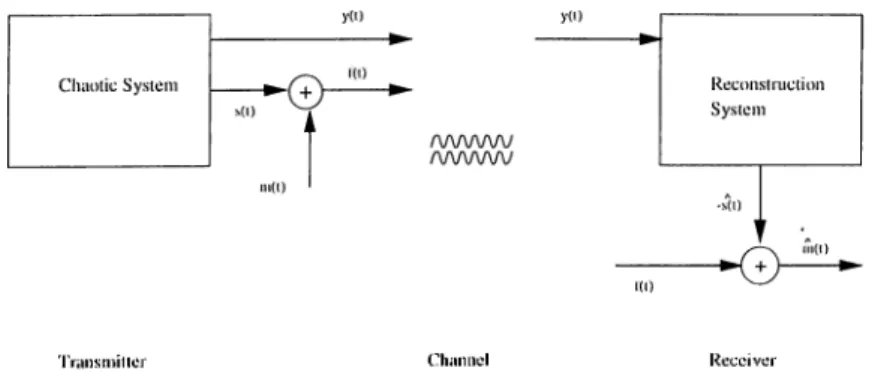
In Figure 4.1, a cornmuniccition system using chaotic signals in modulation is depicted. Here, s(t) and y{t) can be viewed as two states of a chaotic system. We modulate s{t) additively by the message signal m{t) and send the resulting signal f{t) to the receiver end. Also another state y{t) of the chaotic system is directly sent to the receiver end through a different channel. This sigiml is used to reconstruct s{t) which, in turn, is subtracted from f{t) to get ci copy of the original message.

'rrnnsmitter

Figure 4.1; A communication system using chaotic modulation

4.1

S yn ch ron ization by E x p lo itin g th e S ys­

te m S tru ctu re

A common approcich to the synchronization problem is the one that has been proposed in [12, 13]. In this section we will briefly outline their method with an excunple. This method is based on the separation of the system into two subsystems, i.e.. u = ./'(«, io), w = <jiu,to). (4 . 1) (4.2) 31

(4.3) where u G R ” , to G R ’" , / : R ” x R™ ^ R" and ^ : R " x R™ R ”\ At the receiver end, we replicate the second subsystem cind call it the “response system” .

w = g{u,w). (4.4)

VVe assume that the state u of the first subsystem is known and is directly sent to the receiver end. Thus this scheme can be viewed as some of the original state vcU'iables driving the response system, for that rccison our origiiici.1 sj^stem is called the “drive system”. The two systems synchronize if the error = lu — w goes cisymptotically to zero.

lim ew{t) = 0.

¿—>■00 (4.5)

Although the scheme may seem simple at first ghirice, there does not exist an explicit procedure to choose response subsystem to guarcuitee the stability of error system. Moreover there may not exist any plausible choice at all, see

Example 4.1.1 [13] Consider the Lorentz chaotic cittractor system

i = - z), (4.6)

ij = - x z + rx - y, (4.7)

z = xy — bz. (''l-S)

We choose the parameters a - 16 , b - 4, and r = 45.92 so that the system operates in chaotic regime. Then dubbing y and 5; as the response variables, we replicate the response system at the receiver end. Note that the first state variable x{t) is sent as the synchronizing signal.

y = - X Z + rx - y,

z = xy — bz.

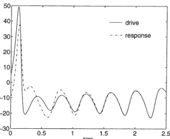
(4.9) (4.10) Below is shown the convergence of the response variable y to the true state of the system for a typical initiiil condition cind for the above choice of parameters.

Figure 4.2: Convergence of y{t) of the response system to y{t) of the drive system for the initial conditions .TfO) = 5 , ;i/(0) = 5 , z(0) = —4, ?/(()) = — fO, and .'¿(0) = 15.

4.2

O bserver B ased S yn ch ron ization

'L'lie synchronization problem described so far can also be addressed from the ol)servation point of view, see [26, 27]. We can take the common synchronizing signal to be the system output of the drive system and the response system can be chosen as a full order observer. Then it becomes possible to use existing observer design strategies for the purpose of synchronization. Besides, tlie system output is not a priori defined for chaotic systems. Hence one can t.ailor an output such that the observer design is facilitated.

Another peculiarity of the chaotic systems is that, since the trajectories always remain in a compact region, we can alwciys find a global Lipschitz bound on the nonlinecvrities involved. Thus the observer proposed in the previous chapter works globally whenever a diffeomorphic transformation to Brunowsky canonical form can be found.

In the following discussion, we first expose the simplification of the observer design for two classes of nonlinear systems, then the nonlinear state transforma­ tion method is applied to Rossler and Lorentz systems and the Chua oscillator.

4.2.1

S y ste m s in L ur’e Form

We consider the class of systems having the structure shown in Figure 4.3. Here L(.s) represents the transfer function of a single-input single-output LTI system cincl ?i(·) : R ^ R is a rnernoryless nonlinearity. This is the well-known Lur’e form which have been heavily investigated [1] and is known to exhibit chaotic behavior for certain cases. Such a system can always be synchronized using a global observer. We assume that L(ii) is a strictly proper transfer function, then we can find an observable realization (A, B, C) of L(s) such that L(s') = C{sl — A)~'^B. Rewriting the system description in state space,

X = Ax — Bn{y), y = Cx,

(4.11) (4.12) we choose the observer as

X — Ax — y = Cx.

i.{y) + l\{y - y ) , (4.13)

(4.14) lence the error dynamics is given by

e = /R.£, (4.15)

where, by the observability of {C,A) , Ac = A - K C can be chosen to be a stable matrix with an appropriate choice of K. The idea is just the design of observer for a system that is linear up to output injection.

Example 4.2.1 Let L(ii) and ?г(·) be L(.s) = - 1 •S'* + ¿¡2 + 1.25s’ ■n(rj) = - k y \y\ < 1 2ky - 2k sgn(?/) 1 < |j/| < 3 3k ssniy) l?/l > 3 (4.16)

with A; = 1.8 . This s.ystem is known to exhibit chaotic behavior for this set of parameters [28]. Realization is given by

0 1 0 0

A = 0 0 1 , B = 0

0 -1.25 - 1 1

, 6' = [ 1 0 0 ]. (4.17)

Below is shown the system’s chaotic behavior cirid the exponential convergence of the observer states to the system stcites when the observer is as described above. The feedbcick gain is chosen as K =

Figure 4.4; (a) The chciotic behavior of the system. (b)-(c)-(d) System and the observer states for :c(0) = [1, —1, —0.1] ^ and :i'(0) = [—2, —2, f]^

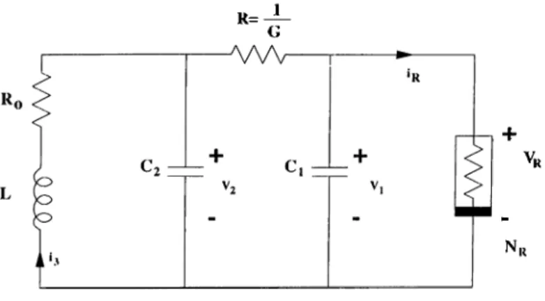
Example 4.2.2 The well-known Chua’s Oscillator circuit [29] can also be rep­

resented in Lur’e form. The state equations are,

Ro 1 Xi 1 G G •^’2 - -T T ^ l “ 7 T®2 + 0 2 ^2 ^2 G G X3 — ^2 •2'’3

J_ '·

where xq = %l , ‘x-2 — '^2 , X3 = > and G = The nonlinear resistor is

described by ir = / (vr), where / : R ^ R is a three segment piecewise linear

R=-Figure 4.5: Cima Oscillator

N„

function given as

= G2X3 + 0.5 (Gri — G2){\x3 -\- E \ — I.T3 — i?|),

and Gy < 0 , G'2 < 0 , jF > 0 are some constants.

If the output is chosen as ij = X3, the system is already a reiilization of Lur’e form with

A = L - 1 X2 0 0 1 G g_ _{, E = 0} C'2 C2 C2 0 _C'lG _ClG _{J - c , .}1 , C = [0 0 1], (4.22) and

n(i/) - Giy + 0.5(G'i — G'2)(|î/ + E\ — \y — E\). (4.2·])

For the simulations, to facilitate the numericcd integration, we define a new independent variable r = and scale Xy by After these changes the system is rewritten as {Ro = 0)

Xy = - /3x2,

X2 = ;ci — X2 + X3,

X3 - ax 2 - a x s - t t/X-'î-'s),

where cv = 9r and 8 = ^ . The linear part of this system is observable if a / 0. We choose the parcuneters as Gy — 0.8 , G 2 = 0.5 , cv = 8 , ¡3 — 11, E = 1, and G - 0.7. When we give excirnples of observer design

(4.25)

by nonlinear state transformation, we will see tlicit the Chua’s oscilhitor also satisfies the necessary conditions for such a diffeornorphic transformation to exist, see Example 4.2.7. Now, we give the simulation results for the above design with K = [ - f , | , -1 ]^.

(b)

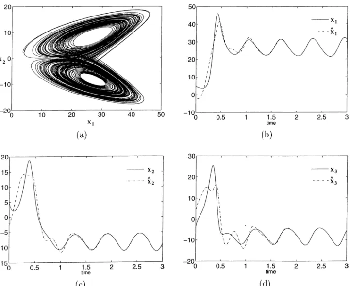
Figure 4.6: (ci) The chaotic behavior of the Chua Oscillator. (b)-(c)-(d) System and the observer states for .t(0) = [0.1, 0.1, 0.1]^ and ¿ (0) = [—2, —2, 2]^

4 .2 .2

Forced O scilla to rs

( 'onsicler an n*'’’ order differential equation

(4.27) where F is a differentiable function of its arguments. Van der Pol and Duff­ ing s,ystems are two examples of the above type displaying chaotic behavior. (Jhoosing ;ri lo and Xi = , i = 1, 2, , we write the state space representation of (4.27) as X = Ax -h Bg{x) -\- Buy (4.28) where A = 0 1 0 0 0 1 0 0 . . . 0 . . . 0 0 1 0 B = 0 1 , ,</(-c) = - F { x ) , u = h{t).

With the choice of output y — x’x, the above representation is in the Brunowsky canonical form of previous chapter. Hence the eigenvalue assign­ ment procedure described therein can directly be applied to design the observer a.s

X — Ax 4- Bg{x) + B u + K{x\ — ;ci). (4.29) 'rtns observer has been used in [30] to design controllers for the purpose of driving following two systems to stable limit cycles.

E x a m p le 4.2.3 As a first example of this type, consider the following forced Van der Pol oscillator;

X 4- d(x^ — 1)7; X = a cos wt + r(f). (4.30) It was shown in [31] that lor various values of d , a and ro, this oscillator exhibits a large variety of nonlinear phenomena, including chaos. This system is in the form given by (4.27) with

Fix , i ) = d{x^ - 1)4’ + ;r. (4.31)

Transforming to stcite space coordinates cind choosing y = rct, we obtain

¿1 = x-z, (4.32)

¿2 = —d{x^ — l ) x 2 — X i + a c o s w t + r(t). (4.33) VVe note that, although the nonlinearity is not globally Lipschitz, the solutions vvliich are of interest to us remain in a bounded convex region ii, of the stcite s|race. Thus a Lipschitz constant can be found by

wliere

7. = sup||V/(,T)||co, xeii

ere, /(.'!’) = —d{x\ — l)xz — Xi- Proceeding this way.

(4.34) l| V /( x )| U = II —2clxiX2 — 1 - d { x j - 1) ind L = supmax{|2da:i.T2 + 1|, \d{xl — 1)|}. (4.35) (4.36) For a pcirticulcir trajectory with d = 6 , a = 2.5 , w = 3, we inspect the plmse portrait of (4.32),(4.33) to set L = 241, then we arbitrarily pick a rcitio r > 1. The first eigenvalue is chosen such that

A ] — A ---~L

V — (4.37)

and the second eigenvalue is given by A2 = rA. Finally the gains are found by ec] iiating

+ k\s + kz = (.s — Aj)(s — A2). (4.38) So, choosing '/’ — 4 and A = —403, we find A2 —16f2 , AT = 2015 , k l — 649636.

One can use this observer to design a state feedback for the purpose of eliminating chaos. Using the bifurcation diagram given in [31], it can be seen that for certain different ranges of the parameter d , the system exhibits chaos or limit cycle. Hence effectively changing the vcilue of this pai'cimeter with state feedback of the form rit) = d f ix j - l)rc2, the system belmvior can be changed from chaos to limit cycle, with the new parameter being d„, = d — dj. For the present example, the bifurcation diagram reveals that when d = 6 , the

system oi^erates in chaotic regime, and for d — 0.5 , we have a limit cycle. Tims, choosing dj = 5.5 we achieve the desired change. When the feedback states are taken from the observer, a nordinear feedback of the form r{t) = 5.5(x'f — l)x2, still drives the system to a stable limit cycle, see [30]. In the simulations both the chaotic regime and the limit cycle are shown. Note that the convergence of the observer stcites to the system states is quite fast while we luive a hrrge overshoot in £2·

( h )

0 .0 4 0 .06

time (d)

Figure 4.7: (a) The chciotic behavior of the Van der Pol forced Oscillator, (b) The limit cycle when the observer-state control is cipplied (c)-(d) System and the observer states for .'c(O) = [0, 0]'^' and ¿(0) = [1, 1]'^.

E x a m p le 4.2.4 Our second example for forced oscillators is Duffing Equation which is used to model different natural phenomena, see [32]. It is described b.y the differential equation

X + üqX + ciix + a,2X^ = <7 cos ivt + r{t). (4.39) The bifurcation structure of this system with respect to pcirameters ciq , rq ,

0,2 can be found in [32].

The state space description of Duffing equation iIS

Xl — X2,

X2 = —aoXi — aiX2 — ci2xi + qcostot + r(t).

(4.40) (4.4f)

Although the observer design scheme of the previous example is quite applicable here, we note that the system becomes a realizcition of Lur’e form when ;ri is chosen as output. Then the observer given by

= X2 + k i ( y - x i ) , (4.42)

£-2 = -cioxi - CI1X2 + k2(y - Xl) - «22/'^ + q cos wt + r(t) (4.43) works globally and converges exponentially to the true states. With appropri­ ate choice of ki and A.2, we can place all the eigenvalues of A — K C on the open left half plane. This is always possible since the pair (C, A) with

A = 0 1

-ao - a i

, C = [ 1 0 (4.44)

is ol)servable whenever ciq ^ 0. The pcirameters cire chosen such tha,t the system operates in chaotic regime, ao = 0.25 , ai = 0.2 , íí2 — 1 , q = 7.5 and w = 1. Then by choosing the gain vector K such that A — K C is stable, we construct the observer (4.42),(4.43). Here we give the simulation results for

i< = [ f · t í)·'· “ ‘<1 ’·(') =

(a)

Figure 4.8; (a) The chaotic behavior of the Duffing system, (b)-(c) System and the observer states for ;c(0) -- [2, 2]'-^ and ;c(0) = [—3, — 1]^·

4 .2 .3

R o ssler and L orentz S y ste m s

E x a m p le 4 .2.5 A common test system for the performance of synchronization schemes is the Rossler system,

;ci = - X2 - X3-, (4.45)

.'C2 = Xi + ax2, (4.46)

= -CX3 + X1X3 + 6. (4.47)

This sз^steın exhibits chciotic motion tor certain range of parameters a > 0 , /> > 0 , c > 0, [13].

We first try y = Xi. Using (2.14),

d Q(x) = -¡ - = - r ax dx Xi -X-2 — X3 —xi — ax2 + CX3 — X1X3 — b 0 0 1 0 -1 -1 — 1 — X3 —a c — xi

which is singular lor a;i = a + c. Thus, the sufficiency conclition of global observability is not met for this choice of output since x = ^ ( x ) is not a globally invertible transformation.

This time, we choose y = X2· Then $(.t) becomes (the constant input b can be

ignored) .T = Tx , (4.48) X2 0 1 0 4>(.t) = xi + ax2 z= 1 a 0 — X2 — X3 T CIX\T oi^X‘2, a — 1 + - 1 and d ^ Qix) = — = T, ax (4.49)

which is always nonsingular, enabling us to define a global diireomorphic state transformation by x = $(a·). In the new domain the state eqiuitions become

¿1 — -'¿2, (4.50)

¿2 = 23, (4.51)

^3 = / ( '0 ^ (4.52)

where

f { z ) = - c z i + (ca - 1)Z2 + { a - c)z3 - az\ - az^ + (a^ + l)ziZ2 + 2:22:3 - «.^1-2-3.