Bernstein series approximation for dirichlet problem

(1)

*Corresponding author, e-mail:nurcan.savasaneril@deu.edu.tr

http://dergipark.gov.tr/gujs

Bernstein Series Approximation for Dirichlet Problem

Nurcan BAYKUŞ SAVAŞANERİL1,*

, Zeynep HACIOĞLU2

1 _{Izmir Vocational School, Dokuz Eylül University, Izmir, Turkey} 2 _{Department of Mathematics, University of Selcuk, Konya, Turkey}

Article Info Abstract

The basic aim of this paper is to present a novel efficient matrix approach for solving the Dirichlet problem. The method converts the Dirichlet problem to a matrix equation, which corresponds to a system of linear algebraic equations. Error analysis is included to demonstrate the validity and applicability of the technique.

Received: 30/06/2016 Accepted: 28/11/2017 Keywords Dirchlet problem Collocation method Bernstein series solution Error analysis

1. INTRODUCTION

The Dirichlet problem is to find a function U z that is harmonic in a bounded domain ( )  2

D R , is

continuous up to the boundary D of D, assumes the specified values U z on the boundary ₀( ) D, where U z is a continuous function on 0( ) D.

Laplace’s equation is one of the most significant equations in physics. It is the solution to problems in a wide variety of fields including thermodynamics and electrodynamics. Today, the theory of complex variables is used to solve problems of heat flow, fluid mechanics, aerodynamics, electromagnetic theory and practically every other field of science and engineering. A broad class of steady-state physical problems can be reduced to find the harmonic functions that satisfy certain boundary conditions. The Dirichlet problem for the Laplace equation is one of the above mentioned problems.

The Chebyshev Tau technique was studied for the solution of Laplace’s equation by Ahmadi and Adibi [1]. The Dirichlet problem was solved for some regions by Kurt et al. [9-11]. Also, Chebyshev polynomial approximation was employed for Dirichlet problem in [12]. The analytic solution for two-dimensional heat equation in some regions was expressed by Baykus Savasaneril et al. [2-4,6]. Chebyshev tau matrix method for Poisson-type equations in irregular domain and error analysis of the Chebyshev collocation method for linear second-order partial differential equations were given by Kong et al. [7] and by Yuksel et al. [13,14]. Gas Dynamics equation arising in shock fronts and solution of conformable fractional partial differential equations by using the reduced differential transform method were studied in [8].

In this paper, we have employed a matrix method, which is based on Bernstein polynomials and collocation points. Let us consider the Dirichlet problem on D

   

0,a  0,b ,

(2)

2 0 0, , _ ( )     z D U z D U U z . (1)

Here, for a point ( , )x y in the plane R , one takes the complex notation 2 z x yi ,U z( )U x y and ( , )

0( ) 0( , )

U z U x y are real functions and

2 2 2 2 2        U

x y is the Laplace operator. Similarly the Dirichlet

problem for the Poisson equation can be formulated as

2

( , )

U G x y (2)

with the conditions defined at the points x_k, y_k for ( _k, _k)D, a_{i j}k_, ,k1,...,t and



_t are constants, 1 1 ( , ) , 1 0 0 ( , )     

 

t k i j i j k k t k i j a U .

Here, G x y are functions defined on ( , ) D. We will find an approximated solution, namely Bernstein series solution of (2) such that

, 0 0 ( , )   

 

n n n n ij i j U x y a B_{i n}_, ( )x B_{j n}_,

 

y (3)

where B_{k n}_, , 0



 k n



are Bernstein polynomials. 2. FUNDAMENTAL RELATION

Let P_{n n}_, be Bernstein series solution of (2). Let us find the matrix form of p_{n n}_, and ( , )_, ,

i j n n i j n n _i _j p p x y      . , n n p can be written as , ( , ) n n p x y B_n( )x Q_n( )y A (4) where 0, 1, , ( ) ( ) ( ) ... ( ) n x  B n x B n x Bn n x  B , ( ) 0 ... 0 0 ( ) ... 0 ( ) 0 0 ... ( ) n n n n B y B y y B y              Q , and A



a₀₀ a₀₁ a₀_n a₁₀ a₁₁ a₁_n a_n₀ a_n₁ a_nn



. Hence, P_{n n}( , )_,i j can be written as

(3)

, ( , )

n n

P x y B_n( )x Q_n( )y A.

On the other hand, B_ni( )x can be written as [5]

( ) i n x  B X( )i ( )x DT (5) where D 00 01 0 10 11 1 0 1              n n n n nn d d d d d d d d d ( 1) , 0 , j i j ij n n i i j d _R j j i i j        _  _{ } _       _  X ( )x  1 x xn_, for X ( )i ( )x , the relation

( )k _ X X ( )x Bk (6) is obtained where B 0 1 0 0 0 0 0 2 0 0 0 0 0 3 0 0 0 0 0 0 0 0 0 0 0 0                      n .

By substituting (6) into (5), we get

B ( )_ni ( )x  X ( )x B i D T . (7) If a similar prodecude is carried out, the relation Q _n( )y Y ( )y D will be obtained as

( ) 0 0 0 ( ) 0 ( ) , 0 0 ( ) Y y Y y y Y y              Y Y ( )y  1 y yn_, D 0 0 0 0 0 0                T T T D D D .

Thus, Y ( )j ( )y can be written as

Y ( )j ( )y Y ( )y B j, (8) where

(4)

B 0 0 0 0 0 0              B B B .

By putting (7) and (8) into (4), we obtain the matrix form of P_{n n}( , )_,i j ( , )x y as

( , ) ,i j ( , )

n n

P x y X ( )x B i D T Y ( )y B j D A. (9)

By substituting (4) and (9) to (2), we obtain fundamental matrix equation as

[ ( , )P x y X ( )x B 2 D T Y ( )y D A R x y( , ) X ( )x B D T Y ( )y B D

( , )

S x y X ( )x D T Y ( )y B 2 D T x y( , ) B D T Y D

( , )

U x y X ( )x D T Y ( )y B D V x y( , ) X ( )x D T Y ( )y D A] G x y( , ). (10) Bu using the collocation points





x y_i, _j



: 0i j, n



in (9), one obtains a matrix ₂ ₂

(n1)  (n 1)

W whose

m-th row, 1 m (n1)2, comes from



,



, , ( 1) 1 1 k l m x y k l m k n n   _ _        . Similarly, G is column matrix such as

 



,



, , ( 1) 1 1 1 m x y_t _l t l m t n m G _n   _ _        

G . Thus, a linear system is obtained as



WA G. (11) We investigate the matrix forms for the conditions in three parts. By using (4) and (9), matrix relations are obtained for the conditions

C A 1 1 , 0 0 0       t _k a_{i j} k i j X (_t) B i D T Y (_t) B j D A _t (12) respectively. Let us write (11) as

C A=G₁

where [G₁_{] 1}_t _t. By combining



W G and ,



_C G, ₁_, it follows a new system _W G; _:

, ; , ₁    _{  } _     W G W G C G . (13)

By using the Gauss elimination method and removing zero rows of augmented matrix _W G; _, if

W

is a square matrix, then the unknown matrix A is obtained as

1 



A W

G

. (14)

The collocation points should be changed such that dim(W) (n1)2. Also, if the columns of W are linearly independent, then the matrix A can be calculated by the pseudoinverse method; that is,

(5)

 

 _  

W W W W (15)

where W is the transpose of W . 

3. ACCURACY OF THE SOLUTION AND ERROR ANALYSIS

We can easily check the accuracy of the solution. When the function P x y and its derivatives are ( , ) substituted in Eq. (1), the obtained equation satisfy approximately;

for ( , )x y (x_q,y_q)



0x_qa, 0y_qb





q0,1, 2,...



,

( _q, _q) ( _q, _q) ( _q, _q) 0

E x y D x y I x y and (E x_q,y_q) 10 kq (k_qpositive integer).

If max10kq 10k ( k positive integer) is prescribed, then the truncation limit N is increased, ( _q, _q)

E x y becomes smaller than the prescribed 10k. The obtained error can be estimated by the function

 

, , 0 0 , ( , ), ( , ) ( , ) N N N r s r s r s E x y a T x y g x y I x y   

 

  .

As E_N( , )x y 0 and N is sufficiently large enough, then the error decreases. Hence, we can determine the accuracy of the solution.

4. NUMERICAL EXAMPLE

In this section, a numerical example has been given to illustrate the efficiency of the method.

Also, we have performed a computer program written on Maple, in order to solve this example.

4.1. Example

Let us consider the following Laplace equation with Dirichlet boundary conditions

2 2 2 2 0 ( ,0) 0 , ( , ) 1 0 (0, ) ( , ) 0 0  _ _           u u x y u x u x K y K u y u K y x K (16)

the fundamental matrix equation for (16) is obtained as

[X ( )x B 2 D T Y ( )y D  X ( )x D TY ( )y B 2 D]A 0. Let the collocation points be the Chebyshev interpolation nodes





1 1 2 1 1 1 2 1 , : 0 , , cos , cos 2 2 2  2 2 2   _ _ _{ }    _{ }                i j i i  i i x y i j n x y n n

(6)

X B 2 D TY (y_j) D  X ( )x_i D TY (y_j) B 2 D

and G is a zero matrix. The condition matrices for ( ,0)u x 0, ( , ) 1u x K  , (0, )u y 0, and ( , )u K y 0 are obtained as , ( ,0) n n i p x X ( )x_i D T Y (0) D A 0 i0,1,...,n , ( , ) n n i p x K X ( )x_i D TY ( )K D A 1 i0,1,...,n , (0, ) n n i p y X (0) D T Y ( )y_i D A 0 i0,1,...,n , ( , ) n n i p K y X ( )K D T Y ( )y_i D A 0 i0,1,...,n

Combining these matrices gives the augmented matrix _W G; _. By calculating the coefficient matrix [ ]A , Bernstein series solutions are obtained for different n values. For N=5, we obtain

X 2 3 4 5 1 6 ( ) 1 _ x x x x x x x , B 6 6 0 1 0 0 0 0 0 0 2 0 0 0 0 0 0 3 0 0 0 0 0 0 4 0 0 0 0 0 0 5 0 0 0 0 0 0                      x , B 36 36 0 0 0 0 0 0 0 0 0 0 0 0 0 0 0 0 0 0 0 0 0 0 0 0 0 0 0 0 0 0                      x B B B B B B , D

 

1 2 3 4 5 1 2 3 4 5 0 1 2 3 4 1 2 3 4 5 1 5 5 1 5 5 1 5 5 1 5 5 1 5 5 1 0 1 0 2 0 3 0 4 0 5 1 5 4 1 5 4 1 5 4 1 5 4 1 5 0 1 0 1 1 1 2 1 3 1                                                                                              K K K K K K K K K K

 

0 1 2 3 2 3 4 5 0 1 1 3 4 1 0 1 4 5 4 4 1 5 3 1 5 3 1 5 3 1 5 3 0 0 2 0 2 1 2 2 2 3 1 5 2 1 5 2 1 5 2 0 0 0 3 0 3 1 4 2 1 5 1 1 5 0 0 0 0 4 0 4                                                                                             K K K K K K K K K

 

0 5 6 6 1 1 1 5 0 0 0 0 0 0 5 0                                  _{ }  _{ }       _ _{  }  _{  }      K  _x D 36 36 0 0 0 0 0 0 0 0 0 0 0 0 0 0 0 0 0 0 0 0 0 0 0 0 0 0 0 0 0 0                        T T T T T T x D D D D D D ,Y 6 36 ( ) 0 0 0 0 0 0 ( ) 0 0 0 0 0 0 ( ) 0 0 0 ( ) 0 0 0 ( ) 0 0 0 0 0 0 ( ) 0 0 0 0 0 0 ( )                      x Y y Y y Y y y Y y Y y Y y

(7)

Y 2 3 4 5 1 6

( ) 1 _

x

y y y y y y

and then, as a result, we get the following error analysis illustrated in figures and tables.

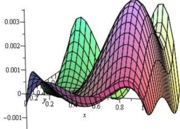
Figure 1. Error analysis for N=5

(8)

Figure 3. Error analysis for N=12

Table 1. Comparison of the error analysis on D that is the boundary of D for different values of N for example D: 0



 x K, 0 y K



x y N=5 N=7 N=9 N=10 N=12 0 1 __{2.4403 10}3

_{1.5690 10}4

_2.161105 _{8.9 10}8 _{1.05 10}7 0 0.9 __{2.0438 10}2

_{1.6914 10}4 __{2.3880 10}5 _{-3.98 10}7 _{-3.90 10}7 0 0.8 __{1.6157 10}3 __{1.1162 10}4 __{1.9550 10}5 _{3.7436 10}8 _{3.7436 10}8 0 0.7 __{7.4720 10}3 __{6.1234 10}4

_{2.195 10}6 _{1.584 10}7 _{1.60 10}7 0 0.6 __{1.6648 10}3 __{1.1537 10}3

_{5.6349 10}6 _{-1.40 10}9 _{9 10}10 0 0.5 __6.4541104 __{8.5508 10}4 __{1.2969 10}4 _{-2.62 10}9 _{-2.6 10}9 0 0.4 __{2.2257 10}3 __{1.9680 10}4 __{1.8373 10}4 _{-1.0338 10}7 _{-1.0362 10}7 0 0.3 __{2.9730 10}3

_{6.9763 10}5 __{4.1595 10}5 _{-9.3988 10}8 _{-9.387 10}8 0 0.2 __{8.0039 10}4 __{1.3218 10}4

_{4.7309 10}5 _{1.6025 10}7 _{1.6031 10}7 0 0.1

_{2.4436 10}3 __{1.0054 10}4 __{1.7810 10}5 _{1.1802 10}8 _{1.1826 10}8 0 0 __{1.6157 10}3 __{1.1162 10}4 __{1.9550 10}5 _{3.7436 10}8

_{3.7436 10}8 It is obvious from Table 1 and Figures 1-3 that the error results get better, as N is increased.

Table 2. Comparison of the error analysis in domain D: 0



 x K, 0 y K



for N=5,7,9,10,12

x y N=5 N=7 N=9 N=10 N=12 1 1 _{2.9900 10}4

1.2359 104 -6.9849 104 7.5900 107 -1.1100 105 0.5 0.5 _{3.9486 10}3 _{-6.7268 10}4

1.5599 105 6.1000 109 -5.2350 108 0.2 0.8 _{1.1137 10}3 _{-1.4905 10}4 _{-6.6864 10}6 _{5.8962 10}6 _{4.2800 10}10 0.1 0.7 _{5.1846 10}3 _-6.6201105 _{-6.5836 10}5 _{-5.7451 10}6 _{1.3544 10}7 0.6 0.6 _{1.0404 10}2 _{-1.2613 10}4

1.1713 106 -3.3402 106 -1.4990 107 0.3 0.2 _{-3.8989 10}3

5.0266 104

6.1778 106 2.5621 105 -9.5388 108 1 0.4 _{-2.0282 10}4

1.9284 104

1.8854 104 3.1996 106 -4.8500 107

(9)

0.8 0.3 _{-6.5765 10} _{-3.0576 10}

_{4.9226 10} _{-1.9480 10} _{4.5170 10}

0.2 0.9 _{6.3258 10}3

1.6659 105 -2.6873 105 -9.7539 107 4.4977 108 0.5 0.7 _{6.1834 10}4 _{-3.5100 10}4 _{-2.7896 10}5 _{-3.7444 10}6 _{2.7140 10}7

The some calculated values of the error analysis are given in Table 2. It is clearly seen that when the values of N increase, error function values rapidly decrease for N=5,7,9,10 and 12.

5. CONCLUSION

In this study, a technique has been developed for solving Laplace’s equation with Dirichlet boundary condition. We introduce a new matrix method depending on Bernstein polynomials and collocation points. Present method provides two main advantes: it is very simple to construct the main matrix equations and it is very easy for computer programming.

CONFLICTS OF INTEREST

No conflict of interest was declared by the authors.

REFERENCES

[1] Ahmadi, M.R., Adibi, H., “The Chebyshev tau technique for the solution of Laplace’s equation”, Appl. Math. Comput. 184(2): 895–900, (2007).

[2] Baykus Savasaneril, N., Delibas, H., “Analytic solution for two-dimensional heat equation for an ellipse region”, New Trends in Mathematical Sciences, 4(1): 65–70, (2016).

[3] Baykus Savasaneril, N., Delibas, H., “Analytic Solution for The Dirichlet Problem in 2-D”, J. Comput. Theor. Nanosci. 15(2): 611–615, (2018).

[4] Hacioglu, Z., Baykus Savasaneril N., Kose, H., “Solution of Dirichlet problem for a square region in terms of elliptic functions”, New Trends in Mathematical Sciences, 3(4): 98–103, (2015).

[5] Isik O.R., Sezer, M., Güney, Z., “Bernstein series solution of linear second-order partial differential equations with mixed conditions”, Math. Methods Appl. Sci. 37: 609–619, (2014).

[6] Kurul, E., Baykus Savasaneril, N., “Solution of the two-dimensional heat equation for a rectangular plate”, New Trends in Mathematical Sciences, 3(4): 76–82, (2015).

[7] Kong, W., Wu, X., “Chebyshev tau matrix method for Poisson-type equations in irregular domain”, J. Comput. Appl. Math. 228(1): 158–167, (2009).

[8] Tamsir, M., Acan, O., Kumar, J., Singh, A.K., “Numerical Study of Gas Dynamics Equation arising in shock fronts”, Asia Pacific J. Eng. Sci. Technol. 2: 17–25, (2016).

[9] Kurt, N., Sezer, M., Çelik, A., “Solution of Dirichlet problem for a rectangular region in terms of elliptic functions”, Int. J. Comput. Math. 81(11): 1417–1426, (2004).

[10] Kurt, N., Sezer, M., “Solution of Dirichlet problem for a triangle region in terms of elliptic functions”, Appl. Math. Comput. 182(1): 73–78, (2006).

[11] Kurt, N., “Solution of the two-dimensional heat equation for a square in terms of elliptic functions”, J. Franklin Inst. 345(3): 303–317, (2007).

(10)

[12] Sezer, M., “Chebyshev polynomial approximation for Dirichlet problem. Journal of Faculty of Science Ege University Series A, 12(2): 69–77, (1989).

[13] Yuksel, G., Isik, O.R., Sezer, M., “Error analysis of the Chebyshev collocation method for linear second-order partial differential equations”, Int. J. Comput. Math. 92(10): 2121–2138, (2014).

[14] Yüksel, G., “Chebyshev polynomials solutions of second order linear partial differential equations”, Phd. Thesis, Muğla University Institute of Science, Muğla, 1-106 (2011).