VERİMLİLİK YANLILIĞI HİPOTEZİNİN GELECEK 11
ÜLKESİ İÇİN İNCELENMESİ
EXAMINING THE PRODUCTIVITY BIAS HYPOTHESIS FOR NEXT 11 COUNTRIES
Gülfer VURALa a Dr. Öğretim Üyesi, İstanbul
Medeniyet Üniversitesi, İktisat Bölümü, İstanbul. ORCID: 0000-0002-7297-7545 E-posta: [email protected] Makale Türü Araştırma Makalesi
Makale Geliş Tarihi
22.12.2019
Makale Kabul Tarihi
18.10.2020
ÖZ
Amaç - Bu çalışmanın amacı Verimlilik Yanlılığı Hipotezinin geçerliliğini Gelecek 11 ülkesi
(Bangladeş, Mısır, Endonezya, İran, Güney Kore, Meksika, Nijerya, Pakistan, Filipinler, Türkiye ve Vietnam) için zaman serileri kullanarak incelemektir.
Yöntem - Ampirik analiz otoregresif dağıtılmış gecikme methodu (ARDL) kullanılarak
yapılmıştır.
Bulgular – Elde edilen sonuçlara gore incelenen zaman diliminde, Verimlilik Yanlılığı Hipotezi
Endonezya, Türkiye ve Vietnam için desteklenmiştir.
Sonuç – Hükümetler, imalat, tarım ve hizmet sektörlerinde verimliliği artıran kapsayıcı ve
sürdürülebilir büyüme politikaları üretmelidir. Verimliliği artırmak için insan sermayesi verimli kullanılmalı ve nitelikli işgücü artırıcı politikalar uygulanmalıdır.
Anahtar Kelimeler: Verimlilik Yanlılığı Hipotezi, Gelecek 11 ülkeleri, Zaman Serileri JEL Kodları: C22, E31, F30
ABSTRACT
Purpose - The purpose of this study is to examine the validity of the Productivity Bias
Hypothesis for the next 11 countries (Bangladesh, Egypt, Indonesia, Iran, South Korea, Mexico, Nigeria, Pakistan, Philippines, Turkey and Vietnam) by using time series.
Methodology – Empirical analysis was performed using the autoregressive distributed lag
method (ARDL).
Findings – The results obtained in the time period analyzed according Productivity Bias
Hypothesis is valid for Indonesia, Turkey and Vietnam.
Conclusions – Governments should consider inclusive and sustainable growth policies that
boost productivity in manufacturing, agriculture and service sectors. In order to increase the productivity, human capital should be employed efficiently and policies to increase skilled labor should be implemented.
Keywords: Productivity Bias Hypothesis, Next 11 Countries, Time Series JEL Codes: C22, E31, F30
1. INTRODUCTION
Exchange rates play an important role for macroeconomic stability and economic growth. Therefore, it is very essential to determine the behavior of real exchange rates and the reasons behind the deviation from equilibrium level. Purchasing Power Parity (PPP) is one of the well-known theories. The theory states that the exchange rate between currencies of two countries is determined as the ratio of the general price level (Halıcıoglu & Ketenci; 2018). Basically, PPP determines equilibrium exchange rates by assuming perfect competition, homogeneity of goods and no trade barriers. Many empirical studies have tested the validity of PPP theory but most of the studies suggest that the theory is not valid.
Several reasons arise for the deviations of exchange rates from the equilibrium level. Productivity differences across countries appear as one of the major factors. Balassa-Samuelson hypothesis that is based
ISSN:
2148-3043
CİLT
VOLUME
20
SAYI
on Balassa (1964) and Samuelson (1964) is also known as Productivity Bias Hypothesis (PBH). The hypothesis suggests that, real exchange rate appreciates when the country is more productive.
Emerging countries are good candidates to test the PBH since these countries experience higher growth rates and relatively faster productivity increases. In this study, the PBH is tested for eleven developing countries that are described as Next 11 or N11. Goldman Sachs defined next generation emerging economies as Bangladesh, Egypt, Indonesia, Iran, South Korea, Mexico, Nigeria, Pakistan, Philippines, Turkey and Vietnam. Main aspect of these countries is the rapid growth rates in recent years. Although PBH is tested for many countries, Next 11 countries are not studied before as an emerging country group. The rest of the paper is organized as follows. Section 1 explains the Productivity Bias Hypothesis. Section 2 has a brief literature review. Section 3 presents methodology and Section 4 has empirical analysis.
2. PRODUCTIVITY BIAS HYPOTHESIS (BALASSA-SAMUELSON HYPOTHESIS)
Balassa (1964) and Samuelson (1964) were independently developed the same hypothesis that is also known as Productivity Bias Hypothesis (PBH). According to the hypothesis, productivity differences across sectors are the only determinants of real exchange rates. Under the assumptions of free labor mobility across sectors, free capital mobility in both across sectors and countries and law of one price in tradable goods sector, productivity increase in tradable goods sector is faster than the non-tradable goods sector. The increase in productivity in the tradable goods sector affects the wages. Therefore the increase in wages in the tradable goods sector is faster than the increases in wages in non-tradable goods sector. In the end, by the free labor mobility assumption the wages in both sectors will be equal. This results in decreases in the profits of firms in the non-tradable sector and then, prices increase and deviations from PPP arise and currency appreciates. The key issue is that productivity changes differently across sectors and across countries. Productivity in the non-tradable sector is smaller and slower than the tradable sector.
Balassa (1964)’s study tested the hypothesis as a first time. Balassa (1964) carried out Ordinary Least Squares (OLS) for nine countries by employing the ratio of the purchasing power parity and nominal exchange rates as the dependent variable and per capita income as the independent variable: PPP/ER=f(Ypc)
Rogoff (1992)’s study was the first paper that investigates the hypothesis in a general equilibrium framework. In the model capital, labor and technolgy are employed as the production factors. Two goods are produced in two sectors; tradable and non-tradable goods sectors. T denotes tradable goods and N denotes non-tradable goods sectors.
YT =AT KTα LT1-α and YN =AN KNβ LN1-β
The demand side is formulated as well. By assuming perfect competition, perfect international capital mobility, perfect mobility of factors across the sectors in the country and law of one price, the study shows that a change in relative price in the non-tradable sector is expressed as the function of a change in the relative productivity of the sectors:
pT/pN =(β/α)aT - aN
Asea and Mendoza (1994)’s study is another important contribution to the theory. They investigate the theory in the long run balanced growth path framework. They developed a model by including utility functions beside demand side of the economy. They found the ratio of sectoral output per capita as the determinant of the relative price of the tradable goods. After their study many researches have focused on relative productivities across sectors. But due to the lack of the sectoral time series data for many countries, the researchers use Gross Domestic Product (GDP) per capita as a proxy for the sectoral productivity.
3. A BRIEF LITERATURE REVIEW
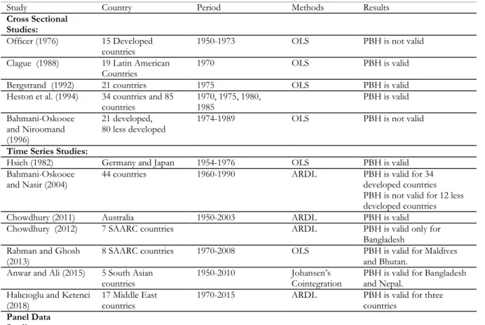
The literature on testing the validity of the PBH is rich but the results are inconclusive. Bahmani-Oskooee and Nasir (2005) present a very detailed literature survey about the PBH. They examine the studies in three parts; cross sectional studies, time series studies and panel studies.
Balassa (1964) conducts the first cross sectional study; Clague (1988), Bergstrand (1992), Rogoff (1992), and Heston et al. (1994) obtained evidence in favor of the hypothesis. However, Officer (1976), Bahmani-Oskooee and Niroomand (1996) rejected the hypothesis.
Hsieh (1982) tested PBH by employing time series data for the first time, for Germany and Japan over the period 1954-1976. The results support PBH. Bahmani-Oskooee and Nasir (2004) examine the hypothesis for 44 countries by employing data from 1960 to 1990. ARDL results suggest that for 32 developed and developing countries the hypothesis is supported, however for mostly less developed 12 countries the hypothesis is not supported. Chowdhury (2011) obtained positive relationship between real exchange rates and productivity differences across sectors over the period of 1950-2003 for Australia. Productivity bias hypothesis is tested for seven South Asian countries by Chowdhury (2012). Support for the hypothesis is obtained only for Bangladesh. Rahman and Ghosh (2013) investigate PBH for eight South Asian countries between the years 1970-2008. PBH gets support for only Maldives and Bhutan. Anwar and Ali (2015) explore productivity bias hypothesis for five South Asian countries over the 1950-2010 period. Findings suggest the validity of the hypothesis for Bangladesh and Nepal. Halıcıoglu and Ketenci (2018) investigate to find support towards the hypothesis in 17 Middle East countries. Empirical findings indicate support for the hypothesis for only three countries.
Asea and Mendoza’s (1994) study is the first study examining PBH in a panel data framework. They developed a general equilibrium model with two countries and two sectors. By using the data of 14 OECD countries covering the period from 1970 to 1985, they found that labor productivity differentials demonstrate international differences in prices. Rogoff (1996) developed a general equilibrium model of Balassa Samuelson hypothesis for the first time. DeLoach (2001) investigated the PBH by examing the relationship between non-tradable goods and output. According to the empirical results of the study there is a long run relationship between non-tradable goods and real output. Egert (2002) investigates the PBH for Czech Republic, Hungary, Poland, Slovakia and Slovenia over the period 1991:Q1-2001:Q2 by time series and panel techniques. But no relationship between productivity growth and price increase is obtained due to the construction of the price indexes. Wang et al. (2016) examine the PBH for 20 developed and 20 developing countries by employing panel cointegration techniques. The results suggest that the PBH holds for developed countries but not for developing countries. Irandoust (2017) explores the validity of the productivity bias hypothesis for New Zealand and its eight major trading partners over the 1995-2011 period. Results suggest support for the hypothesis. Table 1 presents the summary of the selected literature.
Table 1. Selected Literature
Study Country Period Methods Results
Cross Sectional Studies:
Officer (1976) 15 Developed
countries 1950-1973 OLS PBH is not valid
Clague (1988) 19 Latin American
Countries 1970 OLS PBH is valid
Bergstrand (1992) 21 countries 1975 OLS PBH is valid
Heston et al. (1994) 34 countries and 85
countries 1970, 1975, 1980, 1985 PBH is valid
Bahmani-Oskooee and Niroomand (1996)
21 developed,
80 less developed 1974-1989 OLS PBH is not valid
Time Series Studies:
Hsieh (1982) Germany and Japan 1954-1976 OLS PBH is valid
Bahmani-Oskooee
and Nasir (2004) 44 countries 1960-1990 ARDL PBH is valid for 34 developed countries
PBH is not valid for 12 less developed countries
Chowdhury (2011) Australia 1950-2003 ARDL PBH is valid
Chowdhury (2012) 7 SAARC countries ARDL PBH is valid only for
Bangladesh Rahman and Ghosh
(2013) 8 SAARC countries 1970-2008 OLS PBH is valid for Maldives and Bhutan.
Anwar and Ali (2015) 5 South Asian
countries 1950-2010 Johansen’s Cointegration PBH is valid for Bangladesh and Nepal.
Halıcıoglu and Ketenci
(2018) 17 Middle East countries 1970-2015 ARDL PBH is valid for three countries
Panel Data Studies:
Asea and Mendoza
(1994) 14 OECD countries 1970-1985 Seemingly Unrelated
Regression
PBH is valid
Egert (2002) 5 Eastern European
countries 1991:Q1-2001:Q2 FMOLS PBH is not valid
Wang et al. (2016) 20 developed and 20
less developed countries
1980-2014 and
1985-2014 Panel Cointegration PBH is valid for developed countries
Irandoust (2017) New Zealand and its 8
major trading partners 1995-2011 Panel VAR PBH is valid
Source: Author’s own elaboration 4. METHODOLOGY
In this study, empirical analysis is carried out by employing Pesaran et al. (2001) autoregressive distributed lag model (ARDL). The method can be employed when the variables are I(0) and/or I(1) but it is invalid when the variables are I(2). Augmented Dickey Fuller (1979) ADF test is used to determine whether the
variables are I (2) or not. This section briefly explains ADF test and ARDL methodology.
Dickey and Fuller (1979) develops a method to test whether a variable has a unit root or not by employing the model:
𝑦𝑦𝑡𝑡= 𝛼𝛼 + 𝜌𝜌𝑦𝑦 𝑡𝑡−1+ 𝛿𝛿𝛿𝛿 + ∈𝑡𝑡 (1)
In order to avoid serial correlation problem, the Augmented Dickey Fuller test is developed and the test employs the model in Equation 2. Where 𝛼𝛼 is a constant, δ is the coefficient on the time trend, k is the number of lags that has to be determined before applying the test. The null hypothesis of the Augmented Dickey Fuller Test is that the variable has a unit root and the alternative hypothesis is that the variable is generated by a stationary process. The unit root test is conducted under the null hypothesis of β=0 versus the alternative hypothesis of β<0.
∆𝑦𝑦𝑡𝑡= 𝛼𝛼 + 𝛿𝛿𝛿𝛿 + 𝛽𝛽𝑦𝑦 𝑡𝑡−1+ +𝛾𝛾1∆𝑦𝑦𝑡𝑡−1 + 𝛾𝛾2∆𝑦𝑦𝑡𝑡−2 + ⋯ + 𝛾𝛾𝑘𝑘∆𝑦𝑦𝑡𝑡−𝑘𝑘+ ∈𝑡𝑡 (2)
The ARDL methodology is characterized in three steps. In the first step, the existence of the long run relationship between the variables are investigated by F bounds test. Bound testing equation is given in the Equation 3. The appropriate lag lengths are selected according to order selection criteria such as, Akaike Information Criterion (AIC), Schwarz Bayesian Criterion (SBC). After determining the appropriate lag length, the model is estimated by ordinary least square (OLS). In order to determine the existence of cointegration the hypothesis which is given below is tested by Wald test by computing an F statistic. Pesaran et al. (2001) provide two sets of critical values, lower critical values assume that all the variables are I(0) and this implies no cointegration relationship between the variables. Upper critical values assume that all the variables are I(1), and implies cointegration relationship between the analyzed variables. If the computed F statistics is above the upper bound critical values, then the null hypothesis is rejected. If the F statistics is below the lower bound critical value, then the null hypothesis cannot be rejected. If the F statistics is between lower and upper critical values, then no conclusion can be drawn. The null hypothesis and the alternative hypothesis are provided below:
∆Y
t= 𝛼𝛼
0+ ∑
𝑚𝑚1𝑖𝑖=1 1𝑖𝑖𝛼𝛼
∆𝑌𝑌
t-i+∑
𝑚𝑚2𝑖𝑖=0 2𝑖𝑖𝛼𝛼
∆𝑋𝑋
1,t-i+…+∑
𝑖𝑖=0 𝑘𝑘𝑖𝑖𝑚𝑚𝑘𝑘𝛼𝛼
∆𝑋𝑋
𝑘𝑘,𝑡𝑡−𝑖𝑖+ 𝛾𝛾
1Y
t-1+ 𝛾𝛾
2X
1,t-1+…+𝛾𝛾
kX
k,t-1+v
t(3)
H0: 𝛾𝛾
1= 𝛾𝛾
2=…=𝛾𝛾
k= 0 implies no cointegration.
H1: 𝛾𝛾
1≠ 𝛾𝛾
2≠…≠ 𝛾𝛾
k≠ 0 implies cointegration.
In the second step, if the test statistics implies cointegration among the variables, then in the first place, the diagnostic tests of the model that is used for bound testing are performed. ARDL model examining the long run relationship is given in Equation 4.
Y
t= 𝛼𝛼
0+ ∑
𝑛𝑛1𝑖𝑖=1 1𝑖𝑖𝛼𝛼
∆𝑌𝑌
t-i+∑
𝑖𝑖=0 2𝑖𝑖𝑛𝑛2𝛼𝛼
∆𝑋𝑋
1,t-i+…+∑
𝑛𝑛𝑘𝑘𝑖𝑖=0 𝑘𝑘𝑖𝑖𝛼𝛼
∆𝑋𝑋
𝑘𝑘,𝑡𝑡−𝑖𝑖+v
t(4)
In the third step, after obtaining long run relationship among the variables to obtain short run relationship, the model in Equation 5 is employed. ECt-1 is the error correction term and λ is the speed of adjustment
parameter. The error correction term is the lagged value of the residuals of the model in Equation 4. The coefficient of this variable indicates how much of a disequilibrium that occurs in the short run will be corrected in the long run. Positive estimated coefficient of the error correction term means divergence and negative term implies convergence. Therefore, the estimated coefficient has to be negative and significant. When the estimated coefficient is -1 this means that 100% of the adjustment occurs within a period. If the estimated coefficient is 0 this means no adjustment.
∆Y
t= 𝛼𝛼
0+ ∑
𝑛𝑛1𝑖𝑖=1 1𝑖𝑖𝛼𝛼
∆𝑌𝑌
t-i+∑
𝑖𝑖=0 2𝑖𝑖𝑛𝑛2𝛼𝛼
∆𝑋𝑋
1,t-i+…+∑
𝑛𝑛𝑘𝑘𝑖𝑖=0 𝑘𝑘𝑖𝑖𝛼𝛼
∆𝑋𝑋
𝑘𝑘,𝑡𝑡−𝑖𝑖+
λECt-1 +v
t(5)
5. EMPIRICAL ANALYSIS
Following Officer (1976), the link between real exchange rates and productivity differentials is given in Equation 6 by employing the same notation in Vural (2019).
RERt =c0 +c1PRODt + εt (6)
RERt denotes real exchange rate that is obtained by (Pi/Pus) EX. Pi is price level in country i and Pus is price level in US and EX is the exchange rate. PRODt denotes productivity differential. All variables are in natural logarithm.
PRODt=(PRODi/PRODus) PRODi is productivity in country i and PRODus denotes productivity in US. εt is the error term. In order to support the hypothesis, expected sign of the slope parameter c1 is positive. The data counterpart of Pi is the consumer price index in country i. Productivity is measured by real GDP per capita. Equation 6 is estimated for eleven countries; Bangladesh (1986-2017), Egypt, Indonesia, Iran, Korea, Mexico, Nigeria, Pakistan, Philippines, Turkey (1970-2017) and Vietnam (1995-2017). All data come from World Bank, World Development Indicators Database.
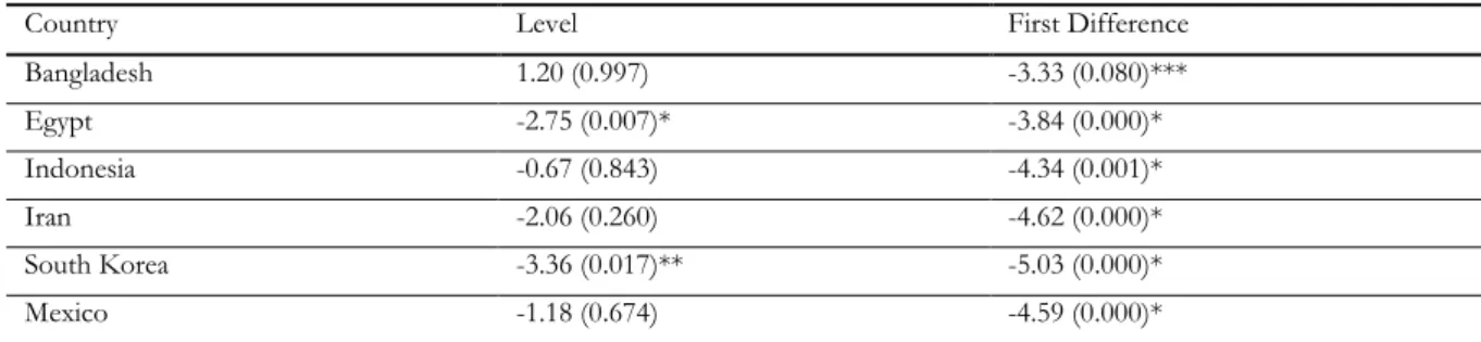
ADF unit root test is conducted to determine whether the variables are I(2) or not. Table 2 and Table 3 present the unit root test results. ADF test results show that the variables are either stationary in level or become stationary in their first difference.
Table 2. Unit Root Test for RER
Country Level First Difference
Bangladesh 1.31 (0.998) -3.93 (0.005)* Egypt 0.54 (0.986) -2.81 (0.068)*** Indonesia -0.82 (0.804) -6.79 (0.000)* Iran 0.59 (0.988) -5.81 (0.000)* South Korea -2.90 (0.053)*** -5.20 (0.000)* Mexico -1.72 (0.284) -6.83 (0.000)* Nigeria -0.15 (0.936) -4.90 (0.000)* Pakistan -1.14 (0.691) -4.73 (0.000)* Philippines -1.48 (0.533) -4.31 (0.001)* Turkey -2.15 (0.031)** -5.45 (0.000)* Vietnam -0.54 (0.863) -2.78 (0.078)***
Notes: *, **, *** Denote the rejection of the null hypothesis (existence of unit root) at the %1, %5 and %10 respectively. The values in parenthesis are the probability values.
Table 3. Unit Root Test for PROD
Country Level First Difference
Bangladesh 1.20 (0.997) -3.33 (0.080)*** Egypt -2.75 (0.007)* -3.84 (0.000)* Indonesia -0.67 (0.843) -4.34 (0.001)* Iran -2.06 (0.260) -4.62 (0.000)* South Korea -3.36 (0.017)** -5.03 (0.000)* Mexico -1.18 (0.674) -4.59 (0.000)*
Nigeria -2.52 (0.117) -4.96 (0.000)*
Pakistan -2.12 (0.239) -4.82 (0.000)*
Phillipines -1.11 (0.704) -3.80 (0.005)*
Turkey 0.57 (0.987) -6.10 (0.000)*
Vietnam 0.63 (0.986) -4.66 (0.001)*
Notes: *, **, *** Denote the rejection of the null hypothesis (existence of unit root) at the %1, %5 and %10 respectively. The values in parenthesis are the probability values.
ARDL representation of the model in Equation 6 is given in Equation 7.
∆RER
t,j= 𝛼𝛼
0+ ∑
𝑚𝑚1𝑖𝑖=1 1𝑖𝑖𝛼𝛼
∆𝑅𝑅𝑅𝑅𝑅𝑅
t-i+∑
𝑖𝑖=0 2𝑖𝑖𝑚𝑚2𝛼𝛼
∆𝑃𝑃𝑅𝑅𝑃𝑃𝑃𝑃
t-i+𝛼𝛼
3RER
t-1+ 𝛼𝛼
4PROD
t-1+v
t(7)
Optimal lag lengths are chosen according to Akaike information criterion. The first stage of the method is the bounds testing that is a Wald statistic (F statistics) and investigates the cointegration relationship between the variables. The null hypothesis is no cointegration among the variables:
H0:𝛼𝛼3=𝛼𝛼4=0
H1:at least one of 𝛼𝛼3, 𝛼𝛼4 ≠0
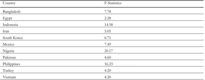
Table 4 shows that only for Egypt the F statistics is smaller than the lower bound and there is no support for the cointegration relationship. Since F Bounds test does not imply cointegration for Egypt, Egypt is eliminated from further analysis.
Table 4. F Bounds Test
Country F-Statistics Bangladesh 7.78 Egypt 2.28 Indonesia 14.58 Iran 5.05 South Korea 6.71 Mexico 7.49 Nigeria 20.17 Pakistan 4.60 Philippines 16.23 Turkey 4.20 Vietnam 4.20
Notes: Null hypothesis of the bound test is no long run relationship exists. LB (low bound), UB (upper bound). 99% LB 4.94, 99 % UB 5.58, 95%LB 3.62, 95%UB 4.16, 90% LB 3.02, 90% UB 3.51
After determining that there is a long run cointegration relationship between the variables Error correction model (ECM) is estimated. Short run parameters are estimated by error correction model (ECM). Equation (8) is the ECM representation of the model.
ECt-1 is the error correction term and λ is the speed of adjustment parameter. Kremers et al. (1992) and Banerjee et al. (1998) demonstrated that a negative and significant ECt-1 can be used as an alternative evidence for cointegration.
∆RERt,j= 𝛽𝛽0+ ∑𝑛𝑛1𝑖𝑖=1 1𝑖𝑖𝛽𝛽 ∆𝑅𝑅𝑅𝑅𝑅𝑅t-i +∑𝑛𝑛2𝑖𝑖=0 2𝑖𝑖𝛽𝛽 ∆𝑃𝑃𝑅𝑅𝑃𝑃𝑃𝑃t-i + λECt-1+wt (8)
Table 5 shows short run results. Table 5 also provides diagnostic tests that indicate reliability of the results. The estimated error correction terms are negative and significant for Indonesia, Iran, South Korea, Nigeria, Pakistan, Turkey and Vietnam. The estimated ECM coefficients are 0.04, 0.01, 0.11, 0.03, 0.01, 0.01, -0.31 respectively. These results imply that about 4%, 1%, 11%, 3%, 1%, 1% and 31% of the disequilibrium in the short run is corrected annually in these countries respectively.
Diagnostic tests show the good fit of the models by R2. Durbin Watson statistics show uncorrelated error terms. Breusch–Godfrey tests show no autocorrelation in the error terms. The CUSUM and CUSUMS2 tests confirm the stability of the model in the countries.
Table 5. ARDL short run results
ECt-1 t-ratio R2 DW RSS χ2N χ2SC χ2H CUSUM CUSUM2
Bangladesh 0.03 5.03 0.29 1.99 0.02 1.01 2.24 1.08 S S Indonesia -0.04 -6.79 0.74 2.01 0.77 5.47 0.06 2.25 S S Iran -0.01 -3.98 0.06 1.82 10.54 1215.76 0.20 0.20 S NS South Korea -0.11 -4.61 0.62 2.00 0.25 0.99 0.92 0.61 S S Mexico 0.00 4.87 0.79 1.94 1.77 9.75 1.06 1.96 S NS Nigeria -0.03 -7.95 0.29 1.83 3.09 33.73 0.25 3.65 S S Pakistan -0.01 -3.80 0.15 1.13 0.47 398.74 10.18 2.08 NS S Philippines 0.00 -7.15 0.63 2.08 0.34 0.52 0.07 4.07 S S Turkey -0.01 -3.64 0.78 1.98 1.91 1.49 0.16 2.46 NS S Vietnam -0.31 -3.89 0.82 2.25 0.01 1.15 0.58 0.98 S S
Notes: RSS means residual sums of squares, DW: Durbin Watson Statistics, χ2N ,χ2SC , χ2H: Lagrange multiplier statistics for normality, residual correlation, heteroscedasticity respectively. These statistics are distributed as chi squared χ2N , χ2SC, χ2H denote Jarque–Bera normality test, Breusch-Godfrey Serial Correlation LM Test, Breusch-Pagan-Godfrey Heteroscedasticity Test respectively. CUSUM: cumulative sum of recursive residuals, CUSUM2: cumulative sum of squares of recursive residuals. S shows
stability, NS shows instability.
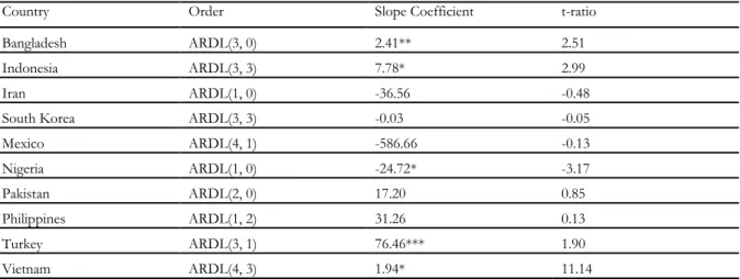
Table 6 shows ARDL long run results. The results indicate that for Indonesia, Turkey and Vietnam the estimated slope parameters are positive and significant supporting PBH. A 1% increase in productivity results in 7.78%, 76.46%, 1.94% appreciation in real exchange rates in Indonesia, Turkey and Vietnam respectively. Although empirical results of the studies of Chowdhury (2012) and Anwar and Ali (2015) support the hypothesis for Bangladesh, in this study the empirical results do not support the hypothesis for Bangladesh. The empirical results depend on the methodology and the selected period of time.
Table 6. ARDL long run results
Country Order Slope Coefficient t-ratio
Bangladesh ARDL(3, 0) 2.41** 2.51
Indonesia ARDL(3, 3) 7.78* 2.99
Iran ARDL(1, 0) -36.56 -0.48
South Korea ARDL(3, 3) -0.03 -0.05
Mexico ARDL(4, 1) -586.66 -0.13 Nigeria ARDL(1, 0) -24.72* -3.17 Pakistan ARDL(2, 0) 17.20 0.85 Philippines ARDL(1, 2) 31.26 0.13 Turkey ARDL(3, 1) 76.46*** 1.90 Vietnam ARDL(4, 3) 1.94* 11.14
Note: *, **, *** Denote the rejection of the null hypothesis at the %1, %5 and %10 respectively. 6. CONCLUSION
Balassa (1964) and Samuelson (1964) investigate the effects of productivity change in sectors on real exchange rate. According to the Productivity Bias Hypothesis (Balassa-Samuelson Hypothesis) the productivity differentials between the countries cause a currency appreciation in a more productive country. Namely, the productivity differences between tradable and non-tradable sectors cause deviations from PPP. In the model, there are two sectors; tradable goods and non-tradable goods. They assume that prices of tradable goods are determined internationally, therefore law of one price is valid. Labor is assumed to be mobile across sectors within the country. If productivity rises in the tradable sector, then wages in this sector increases. Due to labor mobility across sectors, the wages in the non-tradable sector increase as well. At the
end, due to the increases in wages and costs of firms, prices increase and deviations from PPP arise and currency appreciates.
In this study, the Productivity Bias Hypothesis is tested for Next 11 emerging countries. The ADF unit root test confirmed that the analyzed variables are either stationary at level or first difference. The autoregressive distributed lag (ARDL) method of cointegration is used. Empirical findings suggest that the hypothesis is supported for Indonesia, Turkey and Vietnam. The estimated slope coefficient is biggest for Turkey, namely a 1% increase in productivity causes 76.46% appreciation in real exchange rates in Turkey. Therefore, policy makers in Turkey should pay particular attention to increase productivity in the sectors. Rising the competitive power in the high technology and high value added goods export can be a good target to reach this aim. The effects of productivity on real exchange are estimated as 7.78% and 1.94% increase for Indonesia and Vietnam respectively. The failure of the hypothesis in other countries can be due to other macroeconomic variables that the study does not take into account for example governments’ exchange rate policies. In addition, the productivity differentials in tradable goods and non-tradable goods should be considered as well.
Governments should consider inclusive and sustainable growth policies that boost productivity in manufacturing, agriculture and service sectors. In order to increase the productivity, human capital should be employed efficiently and policies to increase skilled labor should be implemented. To increase skilled labor, governments should implement educational reforms beginning with preschool period. Policy makers should increase the budget on research and development. In order for the latest technologies to be used in production, university-industry cooperation should be increased and should be made widespread. Universities, research centers and firms should cooperate to increase research and development investments. Firms should be encouraged to produce and export high value added products to increase the competition power in trade. In order to increase competitive power in the export sector, companies that are concentrated in high technology product export should be provided credits at low interest rates, should be given some subsidies and tax incentives.
REFERENCES
Anwar, S., & Ali, S. Z. (2015). Productivity bias hypothesis: evidence from South Asia. Applied Economics
Letters, 22(17), 1389-1394. DOI: 10.1080/13504851.2015.1034832.
Asea, P. & Mendoza, E. (1994). The Balassa-Samuelson model: a general equilibrium appraisal. Review of International Economics, 2(3), 244-267.
Bahmani-Oskooee, M., & Nasir, A.B.M. (2004). ARDL approach to test the productivity bias hypothesis. Review of Development Economics, 8( 3), 483-488.
Bahmani-Oskooee, M. & Nasir, A.B.M. (2005). Productivity bias hypothesis and the purchasing power parity: a review article. Journal of Economic Surveys, 19(4), 671-696.
Bahmani-Oskooee, M. & Niroomand, F. (1996). A reexamination of Balassa’s productivity bias hypothesis. Economic Development and Cultural Change, 45(4), 195–204.
Balassa, B. (1964). The purchasing-power-parity doctrine: are appraisal. Journal of Political Economy, 72(6), 584-596.
Banerjee, A., Dolado, J.J. & Mestre, R. (1998). Error-correction mechanism tests for cointegration in a single equation framework. Journal of Time Series Analysis, 19 (3), 267-283.
Bergstrand, J.H. (1992). Real exchange rates, national price levels, and the peach dividend. American Economic Review, 82, 56–61.
Chowdhury, K. (2011). Modelling the Balassa-Samuelson Effect in Australia. Australasian Accounting Business and Finance Journal, 5(1), 78-91.
Chowdhury, K. (2012). The real exchange rate and the Balassa–Samuelson hypothesis in SAARC countries: an appraisal. Journal of the Asia Pacific Economy, 17(1), 52-73.
Clague, C. K. (1988). Purchasing power parities and exchange rates in Latin America. Economic Development and Cultural Change, 36, 529–541.
Dickey, D. A., & Fuller, W. A. (1979). Distribution of the estimators for autoregressive time series with a unit root. Journal of the American Statistical Association, 74, 427–431.
DeLoach, S.B. (2001). More evidence in favor of the Balassa-Samuelson hypothesis. Review of International Economics, 9(2), 336-342.
Egert, B. (2002). Investigating the Balassa-Samuelson Hypothesis in Transition: Do We Understand What We See? The Economics of Transition, 10, 273-309
Halıcıoglu, F., & Ketenci N. (2018). Testing the productivity bias hypothesis in Middle East countries. Journal of Economic Studies, 45(5), .922-931.
Heston, A., Nuxoll, D. A. & Summers, R. (1994). The differential-productivity hypothesis and purchasing-power parities: some new evidence. Review of International Economics, 2(3), 227–243.
Hsieh, D.A. (1982). The determination of the real exchange rate: the productivity approach. Journal of International Economics, 12, 355-362.
Irandoust, M. (2017). Symmetry, proportionality and productivity bias hypothesis: evidence from panel-VAR models, Economic Change and Restructuring, 50 (1), 79-93.
Kremers, J.M., Ericsson, N.R. & Dolado, J.J. (1992). The power of cointegration tests. Oxford Bulletin of Economic Statistics, Vol. 54(2), 325-348.
Lawson, S., Heacock, D., & Stupnytska, A. (2007). Beyond the BRICs: A look at the Next11. Goldman Sachs. Retrieved 04.03.2020, from https://www.goldmansachs.com/insights/archive/archive-pdfs/brics-book/brics-chap-13.pdf
Officer, L. H. (1976). The productivity bias in purchasing power parity: An econometric investigation. International Monetary Fund Staff Papers, 23, 545–579.
Pesaran, M. H., Shin, Y., & Smith, R. J. (2001). Bounds testing approaches to the analysis of level relationships. Journal of Applied Econometrics, 16(3), 289–326.
Rahman, M. & Ghosh, S. K. (2013). Productivity bias hypothesis: the case of South Asia. Economics Bulletin, 33(3), 1771-1779
Rogoff, K. (1992). Traded goods consumption smoothing and the random walk behavior of the real exchange rate. Bank of Japan Monetary and Economic Studies,10(2), 1–29.
Rogoff, K. (1996). The Purchasing Power Parity Puzzle. Journal of Economic Literature,34(2), 647-668. Samuelson, P. (1964). Theoretical notes on trade problems. Review of Economics and Statistics, 46, 145−154. Vural, G. (2019). Testing the productivity bias hypothesis for Brazil. Press Academia Procedia (PAP), 10, 68-71.
Wang, W., Xue, J., & Du, C. (2016). The Balassa-Samuelson hypothesis in the developed and developing countries revisited. Economics Letters, 146, 33-38.
World Bank (2019). Retrieved 03.08.2019, from https://databank.worldbank.org/source/world-development-indicators