AN INVENTORY MODEL FOR RANDOMLY
PERISHING GOODS
A THESIS
SUBMITTED TO THE DEPARTMENT OF INDUSTRIAL ENGINEERING AND THE INSTITUTE OF ENGINEERING AND SCIENCE
OF BILKENT UNIVERSITY
IN PARTIAL FULFILLMENT OF THE REQUIREMENTS FOR THE DEGREE OF
MASTER OF SCIENCE
By
Banu Yiiksel September 2000
Ні-> ц о
2 о о <
I certify that I have read this thesis and that in my opinion it is fully adequate, in scope and in quality, as a dissertation for the degree of Master of Science.
Asso tjurler (Supervisor)
I certify that I have read this thesis and that in my opinion it is fully adequate, in scope and in quality, as a dissertation for the degree of Master of Science.
d , C . „ L
Assoc. Prof. İhsan Sabuncuoglu I certify that I have read this thesis and that in my opinion it is fully adequate, in scope and in quality, as a dissertation for the degree of Master of Science.
Assist. Prof. Emre Berk
Approved for the Institute of Engineering and Science:
Prof. Mehmet B ^ay,
Abstract
A N IN V E N T O R Y M O D E L F O R R A N D O M L Y P E R IS H IN G G O O D S
Banu Yüksel
M . S. in Industrial Engineering Supervisor: Assoc. Prof. Ülkü Gürler
September 2000
In this study, we consider an (s, S) ordering policy with backordering for a continuous review inventory system, where the items have a random shelflife. Assuming zero lead time and no decay until the shelflife, we derive the exact expressions for both unit and random batch demand cases with renewal demand arrivals. We present some analytical results on the cost rate function for unit demand case. A detailed numerical analysis is also provided to investigate the performance of the model which incorporates the random shelflife and comparisons with flxed shelflife are given.
özet
R A S S A L R A F O M R U O L A N Ü R Ü N L E R İÇ İN B İR E N V A N T E R P O L İT İK A S I
Banu Yüksel
Endüstri Mühenlisliği Yüksek Lisans Tez Yöneticisi: Doç. Ülkü Gürler
Eylül 2000
Bu çalışmada stoktaki malların raf ömrünün tesadüfi bir değişken olduğu, geri ısmarlamalı ve sürekli gözden geçirilen envanter sistemleri için (s, S) ısmarlama politikası incelenmiştir. Taleplerin yenilenen bir sürece göre geldiği varsayılarak birim talep ve talep miktarının genel bir dağılıma sahip tesadüfi bir değişken olduğu durumlar için uzun vadede ortalama maliyet ifade edilmiştir. Ayrıca, birim talep için maliyet fonksiyonunun analitik özellikleri incelenmiştir. Bu modelin performansını değerlendirmek için sabit raf ömürlü modelle sayısal analiz karşılaştırmaları verilmiştir.
A n a h ta r sözcü k ler: Bozulabilir envanter, tesadüfi talep miktarı, yenilenen sürece göre gelen talep
my parents, grandmother and Mehtap
Acknowledgement
I would like to express my deepest gratitude to Assoc. Prof. Ülkü Gürler for all the encouragement and trust during my graduate study. She has been supervising me with patience and everlasting interest for this research and also for my future career.
I am grateful to Assist. Prof. Emre Berk for his invaluable guidance, remarks and recommendations not only for this thesis but also for my future works.
I am also indebted to Assoc. Prof. Ihsan Sabuncuoglu for accepting to read and review this thesis and for his suggestions.
I would like to express my deepest thanks to Ayten Türkcan for all encouragement and academic support. Without her continuous morale support during my desperate times, I would not be able to bear all.
I would like to extend my sincere thanks to Hande Yaman, Evrim Didem Güneş, ÇağnGürbüz and Rabia Köylü for their keen friendship and helps.
I would also like to thank my home mate Selma Ayşe Özel, my office mates Gonca Yıldırım, Pelin Arun for their understanding.
Finally, I would like to express my gratitude to Ongun Özkaya for his love, understanding and kindness. I owe so much to him in my life for the happiness he brought to me.
Contents
Abstract i
Özet Ü
Acknowledgement iv
Contents V
List of Figures vii
List of Tables viii
1 Introduction and Literature Review 1
2 Inventory Process with Unit Demands and Renewal Arrivals 10
2.1 Notation and Characteristics of the m o d e l ... 13
2.2
Derivation of the Operating Characteristics... 16 2.3 Analytical Properties of ACs,a ... 213 Inventory Process with Batch Demands and Renewal Arrivals 32
3.1 Additional Notation and Basic C h aracteristics...
34
3.2
Derivation of the Operating Characteristics...39
3.3 More Properties on Operating Characteristics
43
4 Numerical Analysis 56
4.2 Numerical Analysis - Batch dem an d... 67 5 Conclusion 72 A P P E N D IX 79 A .l Appendix A ... 79 A .2 Appendix B ...
86
A.3 Appendix C ...88
A .4 Appendix D ... 99 VIList of Figures
Typical cases of the inventory level p r o c e s s ... 15
Possible realizations for fc’th demand a r r i v a l ... 17
Different realizations for 5*(A ) and A *(s) 2.1
2.2
2.3 2.4 Typical Realizations for ACs,a · 2.5 3.1 3.2 30 30 Different Realizations for ACs»(a),Ai^ ^s,a*{s) ... 31Possible cycle realizations with random demand s iz e ... 36
Positive Inventory level process at a demand a r r iv a l... 38
3.3 Negative inventory level process at a demand arrival...
39
3.4 Different Realizations for cost components at 5 = 10 for r = 10,3
44
3.5
Different Realizations for cycle length at S — 10 for r = 10,3 . . .45
3.6 Realizations for
E[r
2]
—5
at 5 = 10 andE[
t]
= 3,10 48 3.7 ylC (5
,5
) with S '= 1 0 ...49
3.8 Different Realizations for cost items at s = - 3 0 for t = 10,3 . . . 50
3.9 Different Realizations for cycle length at s = - 3 0 for T = 10,3 . . 51
3.10 F [ri] for/Xt = 3 , 1 0 ... 52
3.11
Realizations for ACs,s at s = —30 andE[
t]
= 3,10
...53
3.12 Realizations for E[r2] — s at s = —10, —20, —30 and
E[
t]
= 3,10 .53
3.13 Realizations for AC{s,S) atE[
t]
= 1 0 , 3 ...55
4.1 %C vs UjI¡J..T
64
4.2 h{x) vs E[BS] for different batch d istribu tion s... 67A .l Fixed Shelflife vs Random S h e lf lif e ... 103
A .2 Fixed Shelflife vs Random Shelflife-Cont’ d ... 104
List of Tables
1.1
Summary of studies on perishable in v e n t o r y ...9
3.1 E[DAi] values for different batch distributions and order-up levels 46 3.2 l5[ri] value for different batch distributions and order-up levels . . 47
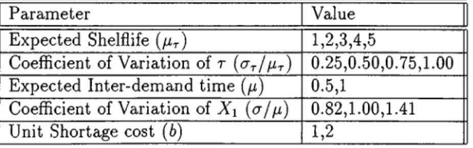
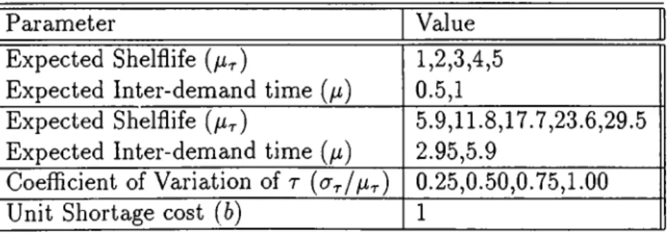
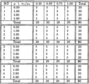
4.1 Experimental Set-up ^ I ...
57
4.2 Sensitivity Analysis f o r / f ,
7
T,6
, /¿T-... 584.3 Summary of sensitivity a n a ly s is ... 59
4.4 Experimental Set-up
# 2
... 604.5 Frequency of experiment settings for unit demand with gamma distributed r ... 60
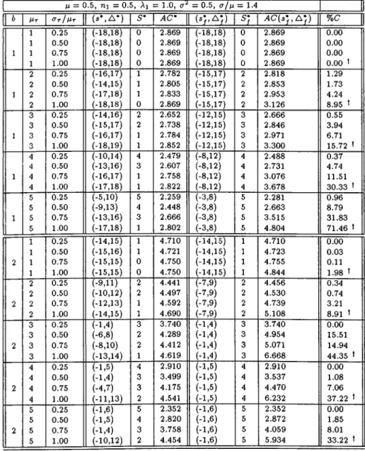
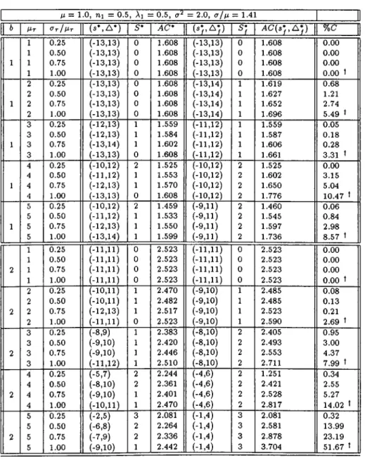
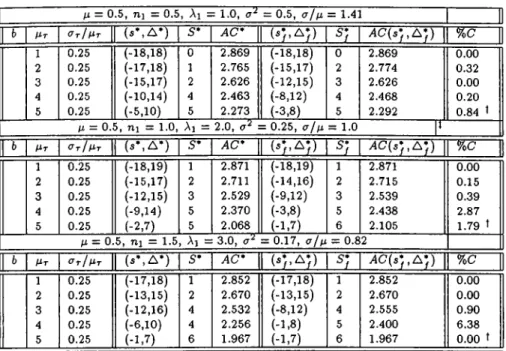
4.6 AC{s*j, Ay) vs AC{s*, A*) for fx = 0.5 61 4.7 AC{s}, A } ) vs AC{s\ A ’ ) for yii = 1.0 62 4.8 y4C(sy, A y) vs v4C'(s*, A*) for/li = 0.5 - Normal Distribution . . . 65
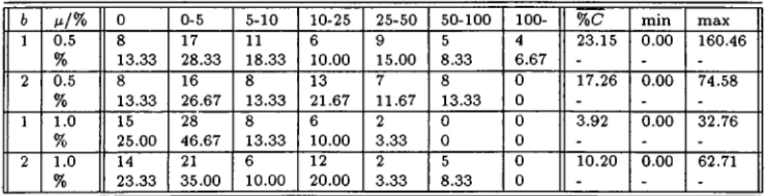
4.9 Frequency distribution for %C with unit demand
66
4.10 Experimental Set-up # 3 ... gg 4.11 Frequency of experiment settings for batch dem ands... 694.12 Frequency Distribution of %C with batch demands
71
A .l ^ ^ (s y , A y) vs A(7(s*, A *) for ^ = 0 .5 -Cont’d ...99
A
.2
A C (5
y, A y) vs ^4(7(5*, A *) for ^ = 0 .5 -Cont’d ... lOO A.3 A C (5
y, A y) vs ACis*, A *) for yu = 1 .0 -Cont’d ...iQl A .4 A C (5
y, A y) vs A C(s*, A ‘ ) for yu = 1.0 - Cont’d ...102
A .5 ^(^(s*,^*) vs ^(^(sy,^^) with = 0 .5 ,1 .0 ...
105
A
.6
AC(s*, S'*) vs A C (sy,5y) with Z)#l,jU = 2 . 9 5 , 5 . 9 ... 106A .7 AC(s*, ,?*) vs A C(sy, 5y) with B D #2,/x = 0 .5 ,1 .0 ... 107
A
.8
AC(s*, 5*) vs ЛС'(б}, 5 ;) with = 2 . 9 5 , 5 . 9 ... 108 A.9 AC(s*, 5*) vs A C (s },5 ^ ) with B Z ) # 3 , / i = 0 .5 ,1 .0 ...109A
.10
AC{s\ 5*) vs AC{s}, S*j) with = 2 . 9 5 , 5 . 9 ...110A .l l A C (s*,5 *) vs A C (s;^,5;) with = 0 .5 ,1 .0 ... I l l
A
.12
AC{s\ S*) vs AC{s}, S}) with = 2 . 9 5 , 5 . 9 ...112
Chapter 1
Introduction and Literature
Review
Inventory analysis is one of the most important areas of application of quantita tive methods. It has been long before recognized that inventory management is a major problem for all companies, whether they are in manufacturing or service fields. The two major objectives of inventory management are maximizing the level of customer service and minimizing the cost of providing such customer service, which are in conflict. The achievement of high service level, ie fewer backorders or fewer lost sales, is accomplished with larger amounts of inventory. Thus, there are two basic inventory decisions to make regarding the two objectives stated above. These are how much to order and when to order.
Starting with the basic EOQ model [
12
], many extensions have been made in the inventory literature to answer the two questions stated above under different circumstances. The uncertainty of demand which is, in fact, one of the major motives for holding inventory is an important and widely focused extension in inventory literature. Some other extensions regarding the physical structures of the inventory systems are positive (random or deterministic) replenishment lead time, the review period (continuous review or periodic review with single period or infinite horizon), backorder or lost sales, continuous replenishment (finite production rate), multiple items or multi-stage.Chapter 1. Introduction and Literature Review
In this study, we consuder a single-item, single-location inventory system. For inventories with single location, single location, unit demand and infinite lifetime, it has been shown that (s,S) type policies are optimal when full backorders are allow ed [37],[13]. With this optimality result, there are many studies which analyze the analysis of (s,S) (or policy for continuous review) type policies and provide algorithms to compute the optimal policy parameters
I«l.|7],i5).i6].|3i|.
However, when the assumption of full backordering is replaced by lost sales assumption, the optimality of (s,S) type policies is not valid anymore. Then, The analysis of the inventory model becomes very complex since the inventory position does not change with a demand arrival when the inventory on hand is zero [
11
]. When more than one order is allowed to be outstanding, even the exact expressions have not been derived yet except (S — 1, S) ordering policy. Also, the optimal policy has not been identified for reasonably general assumptions.Most of the existing models in inventory literature assume that the items have an infinite shelflife and they can be stored indefinitely. However, this assumption assumption may not be applicable in many situations. There are many types of inventories , namely perishable inventories which either deteriorate or become useless after some finite time. When the rate of deterioration is very low or the finite shelflife is relatively long, its effect can be ignored. However, for many practical situations perishability is an important phenomena which should be considered explicitly. Blood products, fresh food, drugs and electronic components are some examples that should be used within their useful lifetime. Volatile chemical substances, radioactive materials and photographic films are examples for continuous decay.
According to these different applications in industry, perishability has mainly three different structures. One of them is the continuous deterioration, in which the items decay with a rate determined by the amount or age of the items. The second one is the fixed shelflife, during which a negligible loss in quality or value is seen, but when the shelflife is reached the items can not be used anymore and should be taken off the shelf. The third structure is similar to the second one
Chapter 1. Introduction and Literature Review
except that the finite shelflife is random.
Nahmias [28] provides a review of inventory models with fixed, random and continuously decaying inventories. Raafat [33] gives a good survey of literature on the models including a continuous deterioration. More specifically, Prastacos
[32] gives an overview on blood inventory management.
The analysis of the models considering the continuous deterioration start with generalizing the conventional EOQ models to include constant or non-constant decay functions. These include the exponential (constant) decay model of Ghare and Schrader [9], Weibull (non-constant) decays of Covert and Philip [4] and gamma (non-constant) decay of Tadikamalla [40].
For this type of inventories, Shah and Jaiswal [39] consider a model deteriorating at a constant rate for a random external demand process with a zero lead time. When a positive lead time is introduced, this problem becomes extremely diff icult since the decay only applies to the inventory on hand but not the inventory position which also includes the inventory on order (Nahmias [28]). Nahmias and Wang [29] consider an exponential decay and develop a heuristic (Q,
7
’ ) policy and show that the cost of heuristic policy is very close to the optimal simulated cost of (Q,r) policy.The studies of fixed shelftime begin with Van Zyl [42] who considers both finite and infinite horizon dynamic programming model with a common shelflife of exactly
2
periods. This study is generalized to ?Ti-period by Nahmias [24] and Fries [8
] independently. However, when m becomes large the computation becomes a severe problem since the analysis is based on a multidimensional dynamic programming. Nahmias [25],[27] provides several approximations for computations.Weiss [44] considers a continuous review model with a fixed shelflife, a Poisson demand process and a zero lead time. In this study, he considers the optimal policies for both lost sales and full backlogging. For the backlogging case, he shows that the optimal policy orders up to S when the marginal shortage cost of not ordering is greater than the optimal expected average cost. So, the optimal policy is a continuous review (s,S) policy with linear shortage cost. For the lost
Chapter 1. Introduction and Literature Review
sales case, he proves the existence of the optimal policy that is of type “never order” or of type “order up to S” when the inventory is depleted. He derives the average cost rate for the lost sales and proves the unimodality of it.
Schmidt and Nahmias [38] discuss a special case of (s, S) policy, namely
(S — 1,5') policy under the existence of a positive lead time and a fixed shelflife perishability for a Poisson demand process. They use the analysis of the 5 dimensional stochastic process corresponding to the time elapsed since the last 5 orders are placed and obtain an explicit expression for the average cost function. Their study is a starting point of the analysis of the perishable items with a positive lead time. But they also comment that it is not possible for anyone to find an optimal policy for perishable inventory model with a positive leadtime.
Chiu [3] proposes an approximation for the continuous review (Q ,r ) model for fixed shelflife inventory with full backordering. With an arbitrary demand distribution and a positive constant leadtime which is assumed to be less than the shelflife of the items, he develops an approximation for the expected number of perishing units per order. He proposes an approximate solution assuming that there is no overshoot at the reorder point r. An iterative procedure for finding only the local optimal (Q ,r ) pair for the proposed approximation is presented since the unimodality can not be proven. The comparison of the proposed approximation with the conventional (Q ,r ) policy and the optimal lost sales policy developed by Weiss [44] is also provided.
Ravichandran [34] consider the stochastic analysis of a continuous review (s, 5) model with a fixed shelflife, a Poisson demand and a random lead time assuming the unmet demand are lost. He derives the explicit expressions for the station ary distribution of the inventory level. This distribution is used to obtain the expected cost rate and to find the optimal reorder level. To avoid the difficulty of keeping track of the inventory level process when the aging of the items begin when they arrive in stock he assumes that the aging of a new batch does not begin until all the units from the previous batch are sold or perish and so he uses a FIFO issuing policy.
Chapter 1. Introduction and Literature Review
shelflife, constant lead time, Poisson demand process and a partial backordering. They assume that the waiting time of customers have a general distribution and customers whose demands are unmet can see how much time is left for the arrival of the next available item. They obtain the marginal density for the one dimensional stochastic process corresponding to the minimal virtual outdating times in the stecuJy state. They also provide the steady state probabilities of the on hand inventory.
Another recent study is by Liu and Lian [19] who consider an (s, S) continuous I’eview model with a fixed shelflife, a general demand process and a zero lead time. They identify a Markov renewal process embedded at two regenerative points of the inventory level process to obtain the average cost rate. They give a mathematical analysis of the average cost rate with respect to s for a fixed S and show that the average cost rate is monotone or convex in s. They also provide a numerical analysis and conclude that min_s C { —s,S) is unimodal with respect to S. By using these analyses they provide an algorithm to find the optimal pair
{s,S) for the decision makers.
Tekin, Gürler and Berk [41] study a time based control policy for continuous review inventory systems with constant shelflife, Poisson demand and lost sales. Assuming a specific aging pattern similar to Ravichandran [34], they analyze the problem under a service level criterion.
Regarding the third type of perishability, the items in a single batch may have a common random shelflife which means that they perish at the same age or a non-common shelflife which means that the items of the same age only have a common remaining shelflife distribution but perish independently of each other.
The first study with random shelflife and random demand process is by Nahmias [26] who considers the periodic review problem. Under the assumption that the order of entering the inventory is preserved for perishing also, he shows that the structure of the optimal policy is the same as that of fixed shelflife for a periodic review. By using a dynamic programming model, he derives the explicit expression of the expected number of perishing items of an order.
Chapter 1. Introduction and Literature Review
exponential shelflife, full backordering and a. zero lead time. Modeling the inventory level as a Markov Process, he explicitly derives the long run expected cost rate function and provides some analytical properties of the cost function.
When an exponential lead time is introduced to (s,S) continuous review policy with Poisson demands and exponential shelflife, Kalpakam and Sapna
[14], assuming one outstanding order, derives the steady state distribution of the inventory level, shortage rate, failure rate, and reorder rate to obtain the average cost rate function by constructing a finite state Markov Process.
Kalpakam and Sapna [15] discuss the (5 — 1 ,5 ) continuous review policy for exponential shelflife and lead times but the demand arrivals form a renewal process. They identify the inventory level as a semi-regenerative process and obtain the steady-state operating characteristics of the model.
Liu and Yang [22] relax the assumption on the number of outstanding orders for the model considered by Kalpakam and Sapna [14] where backorders are allowed. They obtain a steady state distribution for the inventory level and provide an explicit expression for the cost function.
Recently Liu and Shi [17] analyze a continuous review (s ,5 ) model with exponential shelflife and renewal demands. They assume that when a demand occurs, they pick a unit to find a non-perished one until they meet the demand or the inventory is depleted. They provide a simple relation between the the reorder cycle length and expected positive inventory level for the steady state. Then, they use this relation to find the cost rate function in terms of the reorder cycle length. They show that the cost rate function is monotone, concave or convex in the reorder level and either monotone increasing or unimodal in the order up level.
The literature on perishable inventory we reviewed up to this point is based on the assumption of unit demands. But many types of inventories face demands in batches of random size. In perishable inventory literature, there is not much done about batch demands. One of the few studies is by Goh et al. [
10
] who study a perishable inventory system with both demand and supply are Poisson processes with geometrically sized batches, motivated by blood bank inventory.Chapter 1. Introduction and Literature Review
Using a Martingale approach, they obtain the first two moments of the times between the outdates and shortages.
Another study about batch demands is a discrete time model by Liu and Lian [20]. With a zero lead time and full backlogging assumption, they study a discrete time (s,S) perishable inventory model with geometric inter-demand times and batch demand sizes. They construct a multi-dimensional Markov Chain to model the inventory level process. Fi'om the numerical studies they conclude that discrete-time models can be used to approximate the continuous time models.
A recent study again by Liu and Lian [
21
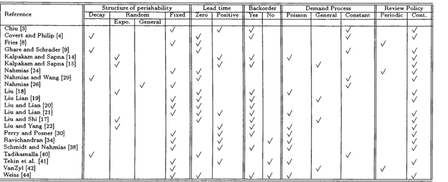
] considers a continuous review perishable inventory system with batch demands. Although they state that they assume renewal demand arrivals, the expressions they provide for the sojourn time at each state of inventory level are valid only for Poisson demand process.Typical classifications of the literature reviewed above may also be seen in Table
1
.1
.As explained above, Weiss [44] has shown the optimality of (s, S) type policy for Poisson demand process, a fixed shelflife and a zero replenishment lead time with backordering. Liu and Lian [19] has also shown that (s, S) type policy is optimal if the time dependent backorder cost is zero with zero replenishment lead time, renewal demand process and fixed shelflife. When the lead time is zero, they also state that (s, S) type policies perform well even if the time dependent shortage cost is not zero since the items on hand always have a common shelflife distribution. With the good performance stated in Liu and Lian [19], we consider an (s, 5 ) ordering policy for items which have a random shelflife and face demands arriving according to a renewal process and zero lead time. We both study the unit and batch demands and derive the operating characteristics. We prove that the cost rate function is pointwise strictly quasi-convex when the shelflife is a continuous random variable and quasi-convex when it is a mixed random variable for the unit demand case. Using the properties of these functions, we give some results on the unimodality of the cost rate function. For batch demand case, we give some key characteristics on the cost rate function. A detailed numerical
Chapter 1. Introduction and Literature Review
analysis is also provided to present how the uncertainty of shelflife affects the optimal policy parameters differently from fixed shelflife and to compare the performance of the model including the randomnes s with the performance of the model considering a fixed shelflife. From the numerical results, it is observed that there is a significant loss by replacing the distribution of shelflife with its mean for both unit and batch demands. To compare with the unit and batch demands, the performance of the model which replaces the distribution with its mean is very poor especially for batch demands with smaller variance of batch distributions.
The rest of this thesis work is organized as follows;
In Chapter 2, we study the (
5
,5
·) continuous review inventory policy and derive the operating characteristics for unit demand case. We give the theoretical and complementary numerical results on the unimodality of the cost function.In Chapter 3, we extend the unit demand case to general batch demands. We give the explicit expressions for the cost function and some key characteristics of the inventory system which helps to understand the behavior of the cost function.
In Chapter 4, we present the numerical results to explore how uncertainty of shelflife and different distributions handling the uncertainty affect the optimal policy and the performance of the inventory system including the uncertainty of shelflife.
This thesis ends with concluding remarks and comments on possible future work in Chapter 5.
Reference
Structure of perishability Lead time Backorder Demand Process Review Policy Decay Random Fixed Zero Positive Yes No Poisson General Constant Periodic Cont.
Expo. General
Chiu [3] x/
y
y
y
y
Covert and Philip [4] v/
y
y
y
y
Fries [8] x/
y
y
Chare and Schrader [9] v/
y
y
y
Kalpakam and Sapna [14]
y
y
y
y
y
Kalpakam and Sapna [15] %/
y
y
y
y
Nahmias [24] x/
y
y
y
Nahmiais and Wang [29] v/
y
y
y
Nahmias [26] x/ x/
y
Liu [18] x/
y
y
y
y
Liu Lian [19] x/
y
y
y
y
Liu and Lian [20] x/
y
y
Liu and Lian [21] x/
y
y
y
y
y
Liu and Shi [17]
y
y
y
y
Liu and Yang [22] v/
y
y
y
y
Perry and Posner [30] x/
y
y
y
y
Ravichandran [34] x/
y
y
y
y
Schmidt and Nahmias [38]
y
y
y
y
y
Tadikamalla [40] v/
y
y
Tekin et al. [41]y
y
y
y
y
VanZyl [42]y
y
y
Weiss [44]y
y
y
y
y
y
C~K CD b C-+-5 c o b Er;C-+-’ CD C-+-C CD CD < CD*Table 1,1: Summary of studies on perishable inventory
Chapter 2
Inventory Process with Unit
Demands and Renewal Arrivals
We consider a single item, single location continuous review inventory system with unit demands, negligible lead time, random inter-arrival times and random shelflife. We assume that the random lifetime of the items in a single batch are common and the perishing time of different batches are independent and identically distributed.
For many inventory systems where the shelflife of the items are assumed to be infinite, (s, S) type policies are optimal for a wide setting of system parameters. But, when the items are perishable the optimal policy has not been identified yet for a general distribution of demands and shelflives. When a Poisson demand process is assumed, Weiss [44] has shown that the optimal policy is of (s, S) type if the replenishment lead time is negligible, the shelflife is constant and linear shortage cost is incurred for backorders. Following this argument, Liu and Lian [19],[21] have pointed out that the optimal replenishment policy would be of (s, S) type for a renewal demand process with fixed shelflife if the replenishment leadtime and time dependent shortage cost are zero. Because of the negligible lead time assumption, at any point the items on hand have a common remaining shelflife distribution and when the the inventory is depleted either by demands or by perishing, it is important to find the order quantity. When a positive leadtime
is introduced, the structure of the optimal policy for a continuous review setting becomes very complex since there may be some old units on hand when a fresh batch arrives and at that point the items on hand do not have a common shelflife distribution. For this type of problem, Schmidt and Nahmias [38] have pointed out that it is unlikely that anyone would be able to find the optimal policy.
In this chapter, we consider the (5 ,5 ) type continuous review policy for the items with a random shelflife. The commonly made assumption of fixed shelflife may not be realistic under some circumstances as mentioned before. For instance, the shelflife of items like fresh food, drugs and chemicals depend on the external factors like heat, temperature, light and moisture. For such cases, it is more reasonable to assume a random shelflife to incorporate the environmental effects. We assume that the items which are subject to the same environmental conditions have the same shelflife, ie the items in a single batch have a common shelflife. From the point of decision maker, he/she usually assumes a fixed, pre-determined shelflife for the perishable inventory on hand and optimizes the system accordingly. However, assuming a fixed shelflife for an item under different circumstances may not be a realistic case as explained above and usually leads to suboptimal solutions for the systems under different conditions. Since a positive lead time adds great complication to the analysis and we do not aim to study the effect of leadtime on the operating characteristics of the policy, we assume that the replenishment lead time is zero. Instead, we aim to find the effect of uncertainty of shelflife on the optimal policy and how different types of distributions handling the uncertainty cause different effects.
We present below the assumptions of the inventory system we are considering:
• The inventory level is reviewed continuously.
• Inter-arrival time of unit demands are independent, identically distributed random variables belonging to a general class of distribution.
• The shelflife of the items in a single batch are identical.
• The shelflives of diffeient batches aie independent identically distributed
Chapter 2. Inventory Process with Unit Demands and Renewal Arrivals
12
random variables with a general distribution. • Back orders are allowed.
• The replenishment lead time is negligible.
• Costs involved in the system are the fixed ordering cost, unit holding cost per time, unit perishing cost, unit backorder cost and unit backorder cost per time.
With the above assumptions of the system, we consider an (s,S) type policy stated as below:
P o lic y : A replenishment order is placed when the inventory level drops to the threshold level, s or below to bring it to S immediately.
The assumption of a negligible replenishment lead time induces an upper bound on s as s < —1 because a policy that orders when the inventory level is non-negative becomes a suboptimal one since the fresh items which arrive instantenously have the risk of perishing while waiting until the next demand arrival, incurring a holding cost at the same time. We should also point out that the inventory level drops to s only by the backordered demands with the induced upper bound on s. So, the policy reduces to a fixed reorder level (s)-fixed order quantity (A ) = S - s policy with a unit demand inventory system. (Sahin [36]).
This study is a generalization of the work by Liu and Lian [19] who consider the (s, S) type continuous review policy for the fixed shelflife case with renewal demand arrivals. They construct a Markov Renewal Process embedded at two regeneration points. These regeneration points are the time that the inventory level is raised up to S units and the time that the inventory level hits -1. Since the demands come according to a renewal process and the shelflife is not Poisson, only the points from the set {5 , - 1 , - 2 , . . . , s + 1 } can be taken as the regenerative points. They obtain the steady state probability of the on-hand inventory. They optimize the system in terms of the reorder-level, s, and order-up level, S. We present a diflFerent probabilistic approach to derive the operating characteristics
of our model. Although we use the same inventory control policy as in Liu and Lian [19], throughout this study we will refer to this policy as (s, A ) rather than (s, S) policy since for unit demand case, the two policies are equivalent with the assumed negligible replenishment lead time [36]. The decision variables for this policy are the fixed reorder level, s and the fixed order quantity, A = S — s.
In the next section, we will introduce the necessary notation to derive the operating characteristics of the system. Since the inventory level process repeats itself at some regeneration points as it will be explained in the next section, the renewal reward theorem will be employed to obtain expected cost rate function.
2.1
Notation and Characteristics of the model
In this section, we introduce the necessary notation and basic characteristics of the inventory model that we consider to derive the operating characteristics of the (s, A ) policy.
Notation
Chapter 2. Inventory Process with Unit Demands and Renewal Arrivals
13
S = order-up level
5
= reorder levelA = S — s, order quantity.
T = Random lifetime of a batch
K = Fixed ordering cost per order
h — Holding cost per unit per time
7
T = Perishing cost per unitb = Shortage cost per unit back ordered
Shortage cost per unit back ordered per time Inventory level at time t
N{t) = Counting process of demands in [0,t)
Xn = Random variable representing the arrival time of ?r’th demand
Fn{t) = P { X n < t )
w
Chapter 2. Inventory Process with Unit Demands and Renewal Arrivals
14
G(t) = P(r < t)
p = Expected inter-demand time
C Ls,a — Cycle length under ( 3 , A ) policy
C Ls,a = Cycle length under ( 3 , A ) policy
CCs,A = Cycle cost under ( 3 , A ) policy
ACs,a — Expected cost rate under ( 3 , A ) policy
HCs,A = Holding cost per cycle under ( 3 , A ) policy
PCs,A — Perishing cost per cycle under ( 3 , A ) policy
BCs,A = Backorder cost per cycle under ( 3 , A ) policy
Cs,A{i) = Total cost accumulated by time t under ( 5 , A ) policy
With this inventory system, we define the points when the inventory level is raised up to 5 = 3 -|- A units as the regenerative points of the system. Therefore, based on our definition of the regenerative points, a regenerative cycle is defined as follows:
R e g e n e ra tiv e C y c le : A regenerative cycle is the time between the two consecutive points at which the inventory level is raised up to 5 =
3
-f A units. We will partition a regenerative cycle into two sub-cycles in order to distinguish the periods during which the inventory level process may behave differently. S u b -c y c le 1: It is the time between the arrival of a new batch of A = 5 - 3 units and the arrival of the first demand after the inventory level drops to 0. That is, it is the time from the beginning of a regenerative cycle until the inventory level drops to -1.S u b -c y c le 2: It is the time interval between the end of sub-cycle 1 and the demand arrival which drops the inventory level to 3 which also completes the regenerative cycle.
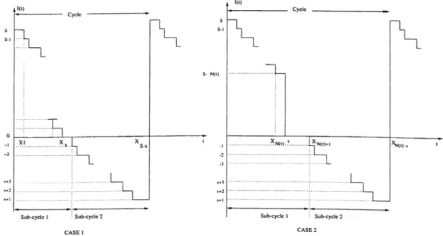
Two typical cases of the inventory process during these regenerative cycles and the sub-cycles are given in Figure 2.1.
In both cases illustrated in Figure 2.1, a regenerative cycle begins with the arrival of a fresh batch of A = 5 -
3
units. The inventory is decreased by one when a demand arrives according to a renewal process. Based on the relationsbetween r and Xs, there exist two possible cases.
In the first case, the inventory is depleted by demands only. This means the shelflife of the batch is greater than the arrival time of the 5” th demand after the regenerative cycle begins. Then, Sub-cycle 1 is then the 5 + 1 demand arrivals provided that S demands occur before the shelfiife of the batch. Sub-cycle 2 begins at the end of Sub-cycle 1 and ends when the inventory level drops to s by the backordered demands which is also the end of the regenerative cycle.
Chapter 2. Inventory Process with Unit Demands and Renewal Arrivals
15
Figure 2.1: Typical cases of the inventory level process
In the second case, some or all of the items on hand perish before being sold. Hence, the shelflife of the batch is smaller than the arrival time of the 5 ’th demand. Sub-cycle 1 is the time interval during which j'V(t) + 1 demands are observed, given that the shelflife is between the arrivals of 7V(T)’th and A^(T) + l ’th demand in a cycle. Similar to the first case explained above. Sub-cycle 2 begins at the end of Sub-cycle 1 and ends when the regenerative cycle ends with —s — 1 backordered demands.
Considering the stochastic processes associated with each possible case of the system, we derive the expressions of the operating characteristics of the system
Chapter 2. Inventory Process with Unit Demands and Renewal Arrivals
16
which will be explicitly explained in the next section.
2.2
Derivation of the Operating
Characteristics
In this section, we will derive the expressions for the operating characteristics, namely the holding cost, the perishing cost and the backorder cost as a function of the decision variables of the policy and the cost parameters given.
In view of the renewal reward theorem, the objective function of the model we are considering is the expected cost rate given as follows;
= l i .
i-oo t E[CL,^¿d
The optimization problem is then stated as
(
2
.
1
)
minACs A = K + + E[HCs a] + E[BCs,a] (
2
.2
) E[CL,,^]When a regenerative cycle and hence Sub-cycle 1 begins, there are two possible events. The first event corresponds to the case where Xi < t. That is, the first demand arrival is observed by which the inventory level decreases to S' — 1. The next event will be another demand arrival or perishing of the items on hand. The second possible event corresponds to the case, t < Xi where all the S items on
hand perish before any demand arrives. The next event will be the arrival of the first backordered demand which will terminate Sub-cycle 1. This argument is generalized to the k'th demand, k £ [ 2 ,3 ,. .., S] as below which is also illustrated in Figure 2.2.
R e a liza tio n 1: (Xk < t) The Eth demand which decreases the inventory level from S—k+1 to S—k arrives before r. Therefore, after the first k—l observed demand arrivals, one more demand arrival and hence a demand interarrival is observed. A holding cost is incurred between the arrivals of it - I ’th and yt’th demand for the 5 - A: +1 items on hand additional to whatever is incurred before.
Chapter 2. Inventory Process with Unit Demands and Renewal Arrivals
17
F igu re 2.2: Possible realizations for k\h. demand arrival
If this realization occurs, then the next event will be either perishing which will occur before k + I ’th demand or a demand arrival which means that Xk+i < r.
R ea liza tion 2: {Xk-i < r < Xk) Perishing occurs between the arrivals of
k - I ’ th and A:’th demand. Thus, at t - t all the S — k 1 items on hand perish, incurring a perishing cost and a holding cost for the period that is held in inventory between Xk-i and r, additional to what is incurred before. When perishing occurs, then the next event will surely be the fc’th demand arrival and this will end Sub-cycle 1.
The following lemma will be used to derive the operating characteristics of the model.
L e m m a 2.1 Let k be a non-negative integer with the convention that Xq = 0 ,/o(x ) = 0, X > 0 and Fo{x) = l , x > 0. Also let IT(·) be the distribution function of t — X·^, and x(·) be the indicator function of its argument. Then,
i) Wr-x,{x) = ft=of{t)G{x + t)dt
ii) E{Xk+\x{Xk < 'T < Xk+\)) = ¡^ o^G{x){fk+i(x) - fk{x))dx
- pf:toG{x)fkix)dx
Chapter 2. Inventory Process with Unit Demands and Renewal Arrivals
18
iv) E [ X k - i x ( X k < r ) ]
v) E[Xk-ix(Xk-i < r < X ,)]
vi) E[Tx(Xk-i < T < A\.)]
fZ o ^fk-i {x)Hr-x, {x)dx IZo xfk -i{x)Hr-x, {x)dx IZo^fk-i{x)G{x)dx Xr
=0
xgix)Fk-i{x)dx L=o x9{x)Fk{x)dx P r o o f: See Appendix A.□
C y c le L en gth :The cycle length under the (
5
, A ) policy is Aa if the items on hand are sold outbefore they perish, that is when X s < t. For this case, the length of Sub-cycle
1
is A5
+A+1
· Otherwise, the cycle length will be Xn(t) -s and the length of Sub cycle 1 will be A ;v(t)+i· For each case. Sub-cycle 2 will be the time needed for the arrival of —5 — 1 units, A _s_i.The following theorem gives the expected cycle length under the (
5
, A ) policy.T h e o r e m 2.1 Denote the expected lengths of Sub-cycle 1 and Sub-cycle 2
E{C Ls,a,i) (knd E {C Ls,a,2) respectively. Then,
as E{C Ls,a,i) = a _ , k=i E{C Ls,a,2) = M - 5 - 1 ) s+A E{C Ls,a) = a ' /*00 __ + X ] / G{x)fk{x)da , - Jxz=0 - S
+
VAT TOO _ Y i / 0{x)fk(x)d:i (2.3) (2.4) (2.5) P r o o f: See Appendix A. □At this point we note that, the expected length of Sub-cycle 1 and Sub-cycle 2 given in (2.3) and (2.4) respectively can be written as the expected number of observed demand arrivals during the sub-cycle multiplied by the expected inter demand time which is similar to the non-perishable case.
C y c le C o st: The cost items incurred during a regenerative cycle are holding, perishing costs which are both incurred during Sub-cycle 1 and backorder costs incurred during Sub-cycle 2 and a fixed ordering cost.
For the cost items incurred during Sub-cycle 1, the stochastic processes associated with the realizations explained above will be used. However, we first give the exact expression for the cycle cost in terms of the given cost parameters and decision variables.
5 N (t)
CCsA = I< + XiXi^s < t)] -b [(7t(F - N (r )) + h Y ^ X i) x { X s > r)]
1=1 2=1
S - s N (t) -s
+ b { - s - 1) + [U) XiX{Xs < r)] + [u; Y XiX{Xs > t)](2.6)
«■=5-1-1 «=yV(T)-|-l
The expression in (2.6) can be used to obtain the expected cycle cost by taking direct expectations. But, as we have explained earlier, for the fc’th demand arrival, there is an associated holding and perishing cost which are independent of what has been incuri’ed up to that demand arrival. So we define a cost function,
Ck which consists of perishing and holding cost associated with the fc’th demand that arrives when the inventory level is positive. Ck {k G [ 1 , 2 , . . . , ¿s -f A] ) is defined as follows with the convention that Xq = 0.
Chapter 2. Inventory Process with Unit Demands and Renewal Arrivals
19
Ck =
h { X k - X k - i ) { S - k + l )
i f T >
(2.7)
( 7
t(5 — A: -f 1) -b h{r — Xk-i){S — k + 1) Xk-i <
t< Xk
With these cost items for each demand arrival, the expected holding costs and perishing cost per cycle can be written as follows:
s + A
E[HC.,^] + E[PC.,^] = ^ E\Ct]
k=\
We next give the theorem which provides the expression for the expected cycle cost.
Chapter 2. Inventory Process with Unit Demands and Renewal Arrivals 20
T h eorem 2.2 The expected cycle cost under the (5, A ) policy is given by the following expression:
,-00
«+A ■’„Ur r<x> _ ^ roo _ E[ CCs,a] = E + h ^ ^ xG{x)fk{x)dx P h ' ^ xFk{x)g{x)da k=i E fOO + 7T ^ / G{x)fk{x)dx + b { - s - 1 ) + k-1 W/J, 5 ( 5 + 1) (2
.8
)P r o o f: According to (2.7) we can write
E [ H Cs,a] = E ^ ( ^ - ^ + l ) № f c - ^ V i x ( X f c < r ) ) ]
k=\ s
+ Y^h{S - k y i ) [E{
t-
AA_ix(AVi < r < AA))]
A;=l
Using the results of Lemma 2.1, we obtain
rcc* __ /*00 __
E [ H Cs a\ = xG{x) fk{x) dx + h J 2 xFk{x)g{x)dx (2.9)
fc=l k=l
For perishing costs incurred in a cycle, we have 5+ A E [ P Cs a] = Y , i ^ { S - k + 1)F;[x(A Vi < t < A ,)] k=l 5+A = X ] 7t(5 - A: + 1) [P{t < Xk) - P {t < A V i )] /c=l
/*00
= '1 2 '^ G{x)fk{x)dx I t''0
k=l (2
.10
)The shortage costs incurred in a cycle consist of the unit backorder costs for
5 - 1
backordered demands and the time dependent backorder costs which areincurred during the time that they are not satisfied.
Then E[CCs,r^] is simply the sum of (2.9),(2.10), (
2
.11
) and the fixed orderingcost, K. □
Theorem 2.1 and 2.2 are then used to construct the objective function given in Equation 2.1 by using the renewal reward theorem. In the next section, we will present the analytical properties of the cost rate function.
2.3
Analytical Properties of
a
In this section, we present the analytical properties of the cost rate function. Since the cost rate function is the ratio of two functions defined at discrete points, it is not so easy to study the analytical properties directly. Therefore, we consider the expected cycle cost and expected cycle length as a function of the decision variables separately.
Due to the discrete structure of the average cost rate function, we need to extend some classical convexity definitions to cover this case. These definitions are given in Appendix B.
We next give the following lemma which states the basic findings for the expected cycle cost and expected cycle length with respect to each decision variable.
L e m m a
2.2
¿) If the shelflife is a continuous random variable, then E is pointwise
strictly concave and E [ C Cs,a] is pointwise strictly convex.
ii) If the shelflife is a discrete or a mixed random variable, E is pointwise
concave and E
[CC'
s,
a]
is pointwise convex.P r o o f:
Let dxi{x,y) be the first order difference of function / with respect to x for a
fixed y and dx^fi^^y) be the first order difference of dxi f { x, y) with respect to x
for a fixed y.
Chapter 2. Inventory Process with Unit Demands and Renewal Arrivals 21
Chapter 2. Inventory Process with Unit Demands and Renewal Arrivals 22 = h S+A+I' ' fOO _ - S + J 2 G{x)fk{x)da roo _ - s + Y ^ G{x)fk{x)da k=i roo _
= /i /
G{X)fs+A+i{x)dx = pP{r >
Xs+A+l)
J X = 0 - hdr\2E{G Ls,a) — dAiE{G Ls,a+i) — dA\E{C Ls,a)
= p [P (r > A^,+a+
2
) - P (r > AA+a+i)]If T is a continuous random variable, then the second order difference is strictl}^ positive, so E{ GLs,a) is strictly concave with respect to A for a fixed s. If t is
a discrete or mixed random variable, then the second order difference is non negative and E{ CLs,a) is concave with respect to A for a fixed s .
ds^E(GLs,A) = E( GLs^i^a) ~~ E( CLs^a) i+A-H = h· - h '' roo _ - s -
1
+ ^ / G{x)fk{x)da roo _ - s + Y G{x)fk{x)da k=i roo _ = J^^^GiX)fs+A+i{x)dx^ = / ^ [ - l + -P (^ > A Va+:)]ds2E{CLs,A) = dsiE{ CLs+i A) - 9si E{ GLs, A)
= P [P{r > Xs+A+2) - P{
t> Xs+A+l)]
This second order difference is positive when r is continuous and nonnegative otherwise, so E{ CLs,a) is strictly concave for continuous r and concave for discrete or mixed random variable with respect to s for a fixed A .
Using these two results, the pointwise concavity of E[ CLsa is proven.
For the cycle cost, we will also consider the first and the second order differences.
Chapter 2. Inventory Process with Unit Demands and Renewal Arrivals 23 OaM C Cs^a) = E{ CCs a+i) - £ ^ { C Cs,a) s+ A + 1
poo
__ s-f-A+l __ = K + h / xG{x)fk{x)dx + h Y / xFk{x)g{x)dx k=l k=lpoo
/"cf q _|_ 1 + T ^ Y G{x)fk{x)dx + b { - s - 1) + wp^—— — — k=i2
^"¡2
^ POO _ _ — K — h Y j xG{x)fk{x)dx — h Y xFk{x)g{x)d. k=\ k=-i - T^Yj
G{x)fk{x)dx + b { - s - 1) + k=i2
POO _ poo _ = h xG{x)fs+A+i{x)dx + h xFs+A+i{x)g{x)dx v/0
»/0
POO -f 7T / G(x)/s-fA+1
{^}dxJo
To examine the second order difference,
5 + A
д/s2E{CCs,¿\) — dAiE{CCs^Ai-i) — dAiE{CCs,A)
POO _ = h xG{x){fs+A+2{x) - fs+A-^l{x))dx J 0 POO _ _
+ h
x{F
s+
a+2
{
x) - Fs+A+i{x))g{x)dx
J 0 POO + 7T / G { x ) { f s + A + 2 { x ) — f s + A + l { x ) ) d x JO — -£'(^s+2
X'’( ^s+A+1
< T < + g-Fix < ^i+ A + i) POO _ _ + / ^(■^s+A+2(a;) - Fs+A+i{x))g{x)dx J 0+ P ( r < AA+
a+ 2 ) - P (
t< A V
a+
i)
Clearly, all the terms are positive for a continuous r and non-negative for a discrete or mixed r. This implies the strict convexity of £^[CCj,a] for a continuous T and convexity for mixed or discrete t with respect to A for a fixed s.
Chapter 2. Inventory Process with Unit Demands and Renewal Arrivals 24 s + A + l dsyE{CCsA) = E{ CCs+i a) - E { C Cs a) roo ^ roo = K -\-h / xG{x)fk{x)dx -\-h YY / xFk{x)g{x)d. k=\
¿=1
+ r G{ x) h{ x) dx + b { - s - 2) + k=l ^ roo _ _ - I< - h Y 2 xG{x)fk{x)dx - h Y Y xFk{x)g{x)dx k=} k=l -7
T V / G{x)fk(x)dx - b { - s -1
) - + ^)) k=i-^0
2
roo _ roo _ - h i f ( ^ x ^ d x ~f· h I x F5
-j-^-j-i i^x^Qi^^x^dx Jo Jo roo + 7T G { x ) f s + A - l · l { ^ ) d ^ - + '^) Jods2E{CCsA) = dsi E{ CCs+i ) - dsi E{ CCsA)
roo _
= h
xG{x){fs+A+2
{x) - fs+A+i{x))dx
Jo roo _ _ p h i x { F syAy2{x) - F syA+i{x))g{x)dx Jo roo+
7T /
G{x){fs+A+2(x) - fs+A+l{x))dx+
Wp JoIf r is a mixed or a discrete random variable, E[ CCs,a] is proved to be conve with respect to s for a fixed A with non-negative second order difference. If r is a continuous random variable, E[CCs a] strictly convex in s for a fixed A .
For both dimensions, the convexity is proven and thus the pointwise convexity.
□
The following two lemmas present the results on the analytical properties of non-linear fractional functions defined at arbitrary non-empty sets. Later, these lemmas will be used with Lemma 2.2 to state stronger properties of the average cost rate function.
L e m m a 2.3 (Generalization of Avriel [1] (pp 156)). Let hi{x) and h2{x) be real valued functions defined on an arbitrary set, X. Let hi{x) be a non-negative
Chapter 2. Inventory Process with Unit Demands and Renewal Arrivals 25
and convex and h^ix) be a positive and concave function on X . Then 4>{x) —
Iii{x)/h2{x) is a quasi-convex function on X .
P r o o f: Since hi{x) is convex on X, we can write by Definition A .l
+
(1
— ^)hi(x2) ^ hi^Xxi “H(1
— X)^2)Vs] € X , y x2 € X ■, and VA G [0,1] s.t x = Axj +
(1
— X)x2 € XSimilarly, since h2{x) is a concave function on X, we can write
(
2
.12
)Xh2{xi) + (1 - X)h2{x2) < h2{Xx-i + (1 - A)a;
2
) (2.13)Vo,'!
6
X, ^X2 € X and VA € [0
,1
] s.t x = Aa;i +(1
- A)x2
^ XNow suppose that f { x) = hi{x)/h2{x) is not quasi-convex. That is, there exists a A
6
[0
,1
] V xi,X2
€ X s.t. x = Axj -)-(1
— A)x2
G X and4>{x) > max [</>(xi), f { x2)] (2.14)
holds which implies that following two inequalities must hold at the same time.
<j){x) > </>(xi)
(j){x) > f { x2)
Combining (2.12),(2.13) and (2.15),
(2.15) (2.16)
Xhi{xi) +
(1
— X)hi{x2) ^ hi{Xxi -j-(1
— A)x2
) /ii(x i)Xh2ixi) T (1 ~ X)h2{^2) /i
2
(Ax‘i -b (1 — A)x'2
) h2{xi)After some algebraic operations, (2.17) leads to the following: ^
1
(3
^2
) ^ hi{xi)h2{x2) h2{xi)
Similarly, combining (2.12),(2.13) and (2.16),
(2.17)
(2.18)
Xh\{xi) +
(1
~ X)h\{x2) ^ hi{Xxi +(1
— A)x2
) ^ /ii(x2
)Chapter 2. Inventory Process with Unit Demands and Renewal Arrivals 26
which results in
hi(x:) ^ hi(x2)
(2.20) /i
2
(x i) h,2{x2)which contradicts (2.18). Since (2.18) and (2.20) can not hold at the same time, there does not exist any A s.t. (2.14) holds, so ^(a;) = /ii(a:)//i
2
(a;) is quasi-convex. □L e m m a 2.4 Let h\{x) and h2{x) be real valued functions defined on an arbitrary
set, X . If hi (x) is a non-negative and strictly convex and h2{x) be a positive and
strictly concave function on X then <f{x) = /ii(x )//i
2
(x) is a strictly quasi-convexfunction on X .
P r o o f: The proof is very similar to the proof of Lemma 2.3 except that we assume that there exists a A G (
0
,1
) for every xi, X2 G X such that (f>{xi) ^ and X = Axi +(1
- A)x2
G X and the following holds:(f>{x) > m a x(^ (xi), (/>(x
2
)) (2
.21
)Then with the same arguments, we end up with a contradiction and conclude that there does not exist any A s.t. (
2
.21
) holds, so (j){x) = hi { x) ( h2{x) is strictlyquasi-convex on X . D
We next give the following theorem which states a strong analytical property of the cost rate function.
T h e o r e m 2.3
t) If the perishing time is a continuous random variable, then ACs,a, is pointwise
strictly quasi-convex.
ii) If the perishing time is a discrete or a mixed random variable, then AC¡a is
pointwise quasi-convex.
P r o o f: Proof of part (¿) follows directly from Lemma
2.2
and Lemma2
.4
. Similarly, proof of part (ii) follows directly from Lemma2.2
and Lemma 2.3.Chapter 2. Inventory Process with Unit Demands and Renewal Arrivals 27
Next, we give the following lemma which presents a generalized statement about the optimality conditions for quasi-convex and strictly quasi-convex functions which are customarily defined in convex sets as it is explained above.
L em m a
2.5
Let X be a non-empty set of discrete points.i) Let h be a real-valued strictly quasi-convex function on X and x* E X be a local minimum of h. Then x* is a global minimum of h on X .
a ) Let h be a real-valued quasi-convex function on X and x* E X be a strict local minimum of h on X . Then x* is a strict global minimum.
P r o o f:
(i) Suppose that x* is a local minimum of h on X.
By Definition A .9 that there exists a non-empty subset A = [x* — k,x* -f A:] C
X , k > 1 such that
h{x*) < h{x) (
2
.22
)Vx e A.
Now, assume that x* is not a global minimum of h on X. Then there exists
X ^ A but X E X such that
h{x) < h{x*)
By the strict quasi-convexity of h, we have VA E (0,1), /i(Ax-b (1 - A)x*) < m ax(/i(x),/i(x*)) = h{x*)
(2.23)
(2.24) Since there exists a A such that Ax -|-
(1
— A)x* E A, we have a contradiction for Inequality 2.22. Then we conclude that every local minimum of h, x* is a globalminimum. D
(ii) Suppose that x* is a strict local minimum of h on X . By definition A .
9
, there exists a subset A = [x* — k,x* -\- k] C X., k > 1 such that Vx € A we have Vx € AChapter 2. Inventory Process with Unit Demands and Renewal Arrivals 28
Suppose that x* is not a strict global minimum of h. Then there exists an
X ^ A but X E X such that
h{x) < h{x*)
For h is quasi-convex in x, we have VA E [0 ,
1
],(2.26)
h{Xx + (1 — A)x*) < m ax(h(x), h(x*)) (2.27) Because there exists a A G [0,1] such that Ax +
(1
— A)x* E A, we have a contradiction for (2.25) by (2.27). So, we conclude that a strict local minimum, X* of /i on X is also a strict global minimum. □We finally give the following theorem about the optimality conditions of the average cost rate function.
T h e o r e m 2.4
i) If the shelflife is a continuous random variable, a local minimum, s* for a
given
A
is a global minimum of the average cost rate function, ACs,a- Similarly,a local minimum
A*
for a given s is a global minimum.ii) The arguments for part (i) are valid for a strict local minimum to be a strict global minimum.
P r o o f: Proofs of part (f) and (u ) are direct results from Lemma 2.5 and
Theorem 2.3. □
With the statements presented in part (i) of Theorem 2.4, if the shelflife is a continuous random variable for a given s or A , the minimum of AC«,a can be
easily found by using any search method applicable to unimodal functions, since we have proven that the local minimum is also a global one. Considering it in two dimensions, an iterative method can be used to find the AC's*,a* hr which if at two consecutive iterations the algorithm finds the same