Experimental investigation of iterative simulation-based scheduling in a dynamic and stochastic job shop

(1)

0

Journal of Manufacturing Systems M Vol. 2a/No. 4

Q 2001

Experimental Investigation of Iterative

Simulation-Based Scheduling in a Dynamic and

Stochastic Job Shop

Erhan Kutanoglu, Dept. of Industrial Engineering, University of Arkansas, Fayetteville, Arkansas, USA lhsan Sabuncuoglu, Dept. of Industrial Engineering, Bilkent University, Ankara, Turkey

Abstract

A vital component of modern manufacturing systems is the scheduling and control system, which determines companies’ overall performance in their respective supply chains. This paper studies iterative simulation-based scheduling mechanisms for manufacturing systems that operate in dynamic and stochastic environments. Also assessed are the issues involved when these mechanisms are used to make higher-level scheduling decisions, such as dispatching rule selection, instead of generation of a full schedule. A typical simulation-based system is outlined and tested under various experimental conditions. Examined are the effects of stochastic events such as machine breakdowns and processing time variations on the system performance, and the effectiveness of the simulation-based approach from the control point of view is evaluated. Finally, different levels of two important factors (look-ahead window and scheduling period) are compared for the iterative approach. Computational results show that, although simulation-based scheduling proves effective when these parameters are properly set, the overall performance diminishes due to the dynamic and stochastic nature of the system, which degrades the multi-pass improvement capability of the simulation runs. Experimental results also support the initial expectation in that frequent updates to the higher-level schedule may not be necessary when these decisions are naturally “adaptive” to the unexpected system changes. Keywords: Scheduling and Control, Simulation Methods and Models

Introduction

Effective production scheduling is becoming an increasingly important component of the supply chain environment that most companies face in today’s competitive markets. Discrete-event simulation is a decision support tool that has been proposed to achieve effective scheduling. During the last decade, a significant body of literature has accumulated in this area, mainly either proposing simulation-based scheduling schemes or testing existing schemes in different settings. Most studies in this

area share two common characteristics: (1) They use static and deterministic environments where all jobs are available for scheduling and no uncertainty is considered. In these cases, simulation is used as a search heuristic for improved scheduling decisions. (2) Simulation is mostly used to assist with constructing a complete schedule of all jobs rather than other types of scheduling decisions; however, a simulation-based scheduling scheme might perform dif- ferently in a dynamic and stochastic environment and/or when the main scheduling decision is different from constructing an off-line static and complete schedule. The main goal in this paper is to investigate how simulation-based schemes perform under dynamic and stochastic conditions through a com- prehensive experimental study when simulation is used to identify scheduling policies rather than to generate a complete schedule.

Two questions are addressed: (1) Are simulation- based schemes still effective in a dynamic and sto- chastic environment? It is already known that the performance of “optimization-based algorithms” used to generate schedules fine-tuned (or even optimal) with respect to deterministic assumptions dete- riorates quickly with the introduction of uncertainty (see Lawrence and Sewell 1997 for processing time uncertainty). This study will show if this is a valid conclusion for simulation-based methods, which are believed to be more flexible, adaptable, and realistic. (2) Is there a difference in the performance when simulation is used to make higher-level decisions? This study evaluates two simulation-based methods: (a) to select the best priority rule among candidates (rule selection), and (b) to fine-tune parameters of a heuristic (parameter tuning). From this perspective, simulation results will not generate a static complete schedule. One can interpret this as a mechanism to separate the higher-level (or more critical) policies

(2)

Journal of Manufacturing Systems Vol. 2a/No. 4 2001 b Time t

T

T T T T

t SP * SP -H- SP +

T

Arrival of job release data SP: Scheduling period LW: Look-ahead window FH: Forecasting horizon

Schematic View of Relations Between Forecasting Horizon, Scheduling Period, and Look-ahead Window

rather than making detailed decisions such as sequencing all jobs and determining start times for operations.

A typical environment is explained where simulation-based schemes can be employed to address the above questions. In this environment, the scheduling and control activity is viewed as an intermediate component of a more global planning system in which decisions regarding production planning and master scheduling are made at a higher level. The scheduling and control level deals with the lower level, short-term decisions using the data provided by the higher levels. Specifically, it is assumed that a planning module provides a master schedule of upcoming jobs (called job release data). The time span of the job release data is called the forecast window. The scheduling module uses simulation runs to make (higher-level) scheduling decisions such as dynamic rule selection and parameter tuning. The length of the simulation runs is usually called the simulation window or look-ahead win- dow, which may or may not equal the forecast win- dow. The time interval between two successive points in time when the scheduling decisions are made is commonly called the schedzding period, which in turn determines the frequency of simulation activation. Simulation-based schemes are usual-

ly used in a rolling-horizon basis; that is, if new four-week job release data are available every week, for instance, and decisions are made for 2 weeks using simulation, then only the first-week decisions are implemented, and at the beginning of the next week new decisions are made for the following four weeks using the fresh job release data (see Figure I). The details of an (iterative) simulation-based mechanism that has been used in past studies are outlined, and the implementation of two specific algorithms for this mechanism is explained. The alternative to simulation-based scheduling will be a well-studied and widely used approach: priority dispatching. Only top-performing priority rules are considered for the problem, job shop scheduling with weighted tardiness objective, which is a surro- gate measure of customer service. These priority rules are dynamic and state-dependent and have inherent flexibility to utilize up-to-date information and accommodate changes. We expect to find somewhat different results from previous findings in which fine-tuned static schedules obtained through simulation were compared against these myopic rules under static and deterministic conditions. The contention is that these rules will work well under highly dynamic and stochastic conditions as compared to simulation-based schemes; however, deteri-

(3)

Journal of Manufacturing Systems Vol. 20Mo. 4

2001

oration of simulation-based schemes may not be so severe because they decide higher-level policies and leave the remaining decisions for later while the dynamics of the system take place.

Literature Review

First, the conceptual studies of simulation-based scheduling are summarized. An early study in this area is by Davis and Jones (1988) who decomposed scheduling problems into a hierarchical decision structure (planning, scheduling, and then control). They proposed a mechanism based on the simulation of each scheduling alternative (priority dispatching rules, routing alternatives, etc). Harmonosky (1990) discussed the implementation issues such as modeling, interface to the physical system, saving the system status for evaluating alternatives, and recovery at decision points. Harmonosky and Robohn (199 1) addressed issues such as the frequency of invoking the simulation mechanism, dealing with the simulation output, data acquisition, and interface problems. In her later work, Harmonosky (1993) analyzed two key issues: (1) the simulation run length and (2) the type of simulation (deterministic versus stochastic due to

machine breakdowns). In another study,

Harmonosky and Robohn (1995) investigated the effects of different manufacturing systems on the computational time of simulation runs. The purpose in this paper, though, is not to address these issues; it is assumed that simulation is a viable approach from these perspectives.

Because two decision types (rule selection and parameter tuning) are the focus, the review mainly concentrates on studies that investigated these areas. Most simulation-based methods use a simulation run for each priority rule in a set of candidate rules, and then select the best among them. An early study in this area is by Wu and Wysk (1988, 1989), whose experimental results showed that when simulation run length is accurately determined according to environmental conditions and objectives, then the approach is very effective. After observing the draw- backs of this study where the simulation window coincides with the constant scheduling period Ishii and Talavage (199 1) proposed variable-length, state- dependent scheduling intervals and simulation windows. The simulation experiments showed that using a scheduling interval defined based on the system

transient state improves the performance over using a constant scheduling interval, which has a very unstable performance as compared to single-pass rules. The results also showed that the performance becomes poorer than for the single-pass algorithms if the scheduling intervals are not accurately determined. After observing the advantages of switching rules in each time period Ishii and Talavage (1994) tested the idea of using a different rule on each machine in each period. Cho and Wysk (1993) developed a neural network model to generate alternative dispatching rules based on the current system status, which are then evaluated by multi-pass simulation. Aytug, Koehler, and Snowdon (1994) also considered a rule-selection algorithm strengthened with a genetic algorithm-based machine learning scheme in a parallel machine setting with flow-time objective. Aytug et al. (1994) reviewed the relevant machine learning literature. It should be noted that the current study fills some research needs (testing in dynamic and stochastic job shops) identified by Aytug, Koehler, and Snowdon and Aytug et al.

The second area where iterative simulation runs are used is what is called parameter tuning, where multiple simulation runs are conducted to tune parameter(s) of an algorithm. An early study by Vepsalainen and Morton (1988) proposed an iterative approach called lead time iteration (LTI) that makes repeated simulation runs to find more consistent queue (waiting) time estimates that are used in priority index calculation. Kiran, Alptekin, and Kaplan (199 1) proposed afeedback heuristic, where a series of schedules is generated using job-based priorities that are smoothed at every iteration using the respective job’s contribution to the performance measure and the job’s priority in the previous iteration. Experiments conducted in static and dynamic flexible manufacturing environments showed that the iterative simulation mechanism can be very useful as compared with single-pass rules.

Ovacik and Uzsoy (1994) presented several rolling horizon procedures to minimize maximum lateness on a single machine in the presence of sequence-dependent setup times. Although not simulation-based the study is reviewed here because it addresses the issues of interactions between plan-

ning horizon and forecast window. The study showed that when forecast window and planning horizon parameters are appropriately selected the proposed rolling horizon procedures outperform the

(4)

earliest due date rule. In a related study, Church and Uzsoy (1992) analyzed several rescheduling policies for dynamic single-machine and parallel-machine problems with the maximum lateness objective. Experimental results showed that periodic scheduling (that is, revising decisions every scheduling period) is very useful when the jobs arrive in batch- es periodically to the system and the scheduling period coincides with the batch interarrival time. In the case of dynamic and continuous arrivals, the benefit of extra scheduling diminishes rapidly.

All studies reviewed so far assume a deterministic (no stochastic events other than dynamic job arrivals) shop environment. Although there are numerous studies that investigate reactive scheduling, rescheduling, and robustness under uncertainty, there are only a few simulation-based studies that consider stochastic shop conditions. Kim and Kim (1994) proposed a simulation-based, real-time scheduling mechanism that evaluates various dispatching rules for a given job set and selects the best one for a given criterion. The best dispatching rule is used until the difference between the actual performance (under urgent job arrivals and machine breakdowns) and the estimated performance exceeds a given limit (called the performance limit); then, a new simulation is performed with the remaining operations, and a new rule is selected. Tayanithi, Manivannan, and Banks (1993a, 1993b) and Manivannan and Banks (1992) proposed an integrated scheduling and control system that com- bines simulation and knowledge-based concepts to perform an analysis of interruptions in the form of machine breakdowns and rush orders in a flexible manufacturing system. When a control decision can- not be obtained readily from the knowledge base, the alternative actions are evaluated using the simulation mechanism.

From the reviewed literature, it is known that static complete schedules (simulation-based or optimization-based) that do not leave any room for dynamic adaptability perform poorly in the face of disruptions. To the best of our knowledge, there is no single study that (1) uses simulation-based approach to decide high-level policies in a dynamic and stochastic job shop environment, and (2) analyzes them using an extensive experimental study under common conditions that test not only levels of stochastic disruptions (machine availability and processing time variation) but also investigate their interactions

Journal of Manufacturing Systems Vol. 2a/No. 4

2001

with method-specific parameters such as look-ahead and scheduling windows. This study fills this void and even addresses several issues that were raised in previous studies as future research directions: job shops instead of single machines or flow shops, processing time variation, and machine availability (together), and so on. Finally, the study shows whether the believed flexibility of simulation-based systems would hold under dynamic and stochastic conditions or not.

Iterative Simulation-Based Scheduling

A dynamic job shop scheduling problem is considered in which some information about future jobs is available for a certain period of time. The information on these soon-to-arrive jobs becomes available periodically; that is, certain characteristics of jobs that will be released to the shop floor are known, say, every week. The planning module, shown by the “plant controller” in Figure 2 creates the job release data (or master schedule). The job release data consists of

l job arrival times that will occur during the next forecast horizon;

l job characteristics such as due dates, job weights, routing information (that is, number of operations, best estimates of processing times, machines that each job visits).

A typical simulation-based decision support to handle this type of scheduling problem is shown in Figure 2. The plant controller lays out the job release data and the managerial objective(s) to the Parameter Selector (PS) and the Iterative Simulation Mechanism (EM). The current shop sta- tus is fed back to the ISM and Parameter Selector by the execution and control module, called the “shop controller” The parameter selector determines the look-ahead (or simulation) window, the scheduling period (SP) or planning horizon, and other parameter values that are used in the ISM algorithm. This is done by examining the current shop status, the job release data, and the objectives (the study in a way provides additional insights for the PS to determine what might work in different conditions). The ISM activates the iterative scheduling algorithm using the provided information. The ISM initializes each iteration (or simulation run)

(5)

Journal of Manufacturing Systems Vol. 2oINo. 4

2001

I --I--

Job release data, objectives, etc Job release

data, objectives

Look-ahead window,

Iterative simulation

Current shop status Scheduling decisions

Figure 2

Schematic View of Simulation-based Iterative Scheduling System

with the current system status, and same dynamic events are generated by using the job release data in each iteration. The objective(s) set by management serve as performance measure(s) in the simulation runs. The simulation run length (called the “simulation window”) is determined by the look-ahead window parameter provided by the PS. The scheduling period defines the frequency of normal ISM invokes (regular scheduling period). Although the ISM can also be activated in case of unexpected events such as machine breakdowns, this option is left for a future study.

It is implicitly assumed that the ISM consists of a somewhat detailed simulation model of the real system. The ISM uses this model to mimic the real-life system and evaluate the alternative scheduling policies by running the model. From this perspective, the ISM is flexible in terms of the variety of policies that it can test. More specifically, the ISM can be employed for many decision types such as:

l Best-rule selection

l Priority update (or parameter tuning) l Constructing a complete schedule

l Reactive scheduling and control policy determi- nation

In the current ISM implementation, the first two of these decisions will be considered. A specific algorithm is implemented for each decision:

l Multi-pass Rule Selection Algorithm l Lead Time Iteration Algorithm

These algorithms are described in detail in the following subsections.

Multi-pass Rule Selection Algorithm

Many researchers have studied priority dispatching rules for more than three decades. The major conclusion that can be drawn from these studies is that there is no single rule that yields the best performance in all conditions and that the performance of a rule is highly affected by the operating conditions and the managerial objective(s). Therefore, changing a dispatching rule over successive time periods based on the current system state, the performance measure, and the current information about the future events can improve overall performance over using a single rule for the entire planning horizon. One issue addressed in this study is to test the effectiveness of this vu/e switching approach as a high-level decision not only in dynamic but also in stochastic environments. Some existing studies that consider similar approaches are reviewed in the previous section (Wu and Wysk 1988, 1989; Ishii and Talavage 1991; Cho and Wysk 1993).

In this specific implementation of this approach, there is a set of candidate rules, each of which can be applied in the shop for the given performance measure (weighted tardiness in this case). The candidate rules can be determined by analyzing their past performances. At each decision point, a new series of simulation runs is performed using each of the candidate priority rules in each run. At the end of each iteration, the performance measure is recorded for that rule, and the rule is selected that produces the best performance for the current look-ahead window. This rule is applied in the system until the next decision point, which is defined by the new information arrival (job release data, see Figure 3).

Because the weighted tardiness job shop problem is examined, the following specialized rules in the candidate set are considered: Apparent Tardiness Cost (ATC), Bottleneck Dynamics (BD), Cost OVER Time (COVERT), Modified Operation Due Date (MOD), and Weighted Shortest Processing Time (WSPT). Notation and definitions of the rules are given in Table 1. WSPT is selected because it yields good performance for tardiness measures in highly

(6)

Journal of Manufacturing Systems Vol. 2a/No. 4 2001

Rule 1 Rule 2 Rule 3

*

Time

f t t t t t

Arrfval of job release data SP:Scheduling period

Figure 3

Schematic View of Candidate Rule Set and Implementation of Rule Selection Algorithm

loaded shop conditions. COVERT (Carrol 1965) and MOD (Baker and Kanet 1983) are two rules for min- imizing the unweighted tardiness. ATC is similar to COVERT, but it utilizes exponential cost function (urgency factor) instead of linear (Vepsalainen and Morton 1987). BD has been developed as an exten- sion of ATC, with the primary difference in the resource usage computation (Morton and Pentico

1993). The resource usage in the denominator of the formula is calculated by summing the terms (resource price times operation processing times) over the remaining operations for the job under con- sideration. The resource price of a machine k at time t (l&(t)) is based on both the current jobs in the queue and the overall utilization, as shown below:

Lx(f)

where Lk(t) is the current queue length, U,,(t) is the urgency factor, (wu),, is the average delay cost, and pk is the average utilization of the machine. (For a broad discussion of the rules, including BD, refer to Kutanoglu and Sabuncuoglu 1999.)

Lead Time Iteration

Some priority rules such as ATC and BD involve parameters that need to be estimated or tuned. It is well known that the performance of these scheduling rules depends on the right setting of these parameters. Specifically, ATC and BD indices use waiting

Table 1

Priority Dispatching Rules in Candidate Rule Set for Multi-pass Rule Selection Algorithm (priorities are calculated for job i waiting for

operationj at machine k at time t)

Prioritv Rule Descrintion WSPT (Weighted Shortest wspTj = $ Processing Time) rl MOD (Modified Operation Due Date) COVERT ATC g?tt leneck Dynamics)

I

4 -

,=t+iYq

+

P,U)

-

P, - t w,xexp -~ K~,vx %(t) = Nomenclature: Weight of job i

Processing time of operation j of job i

Arrival time of job i to the shop Due date of job i

Number of operations of job i

Estimated waiting time of job i for operation q

Average operation processing time

Resource price of machine k for operation q

Constant coefficients

time estimates. One traditional approach is to use a constant multiplier (lead time constant) times pro- cessing time as a waiting time estimate (Vepsalainen and Morton 1987). In general, single-pass versions of ATC and BD employ this approach. To further improve the performance, there are two alternatives: l Several alternative values for the lead time con-

stant are evaluated, and the one which produces the best performance measure is selected. l Lead time iteration (LTI) estimates the waiting

time of each individual operation iteratively using realized waiting times in simulation runs. Waiting time estimates that produce the best estimated performance are used in the implementation of the rule.

(7)

Journul of Manufacturing Systems Vol. 2a/No. 4

2001

In this study, the second approach is employed because it revises the individual waiting time estimates independently by using realized waiting times in previous iterations. Therefore, it is expected that it should perform at least as well as the first alternative for the same number of simulation iterations. LTI starts with initial waiting time estimates set as in traditional estimation method, and smoothes the estimated and the actual waiting time estimations at the end of each iteration for the next iteration. The steps of the algorithm are as follows (for the original version of LTI, see Morton and Pentico 1993):

Step 1. Set iteration number II at 1. Initialize esti- mates (used was three times the processing time, IVV( 1) = 3 X pu) for each job on hand and jobs that will arrive during the look-ahead window. Step 2. Perform a simulation using ATC (or BD). Step 3. Record the performance measure obtained and the actual waiting times (Qijcn)) for iteration n.

Step 4. If a termination condition is satisfied, go to Step 7.

Step 5. Compute the new estimates:

where CY is a smoothing parameter between 0 and 1 (0.5 is used in the experiments).

l Step 6. Increase the iteration number n by 1, and go to Step 2.

l Step 7. Report the best performance measure and corresponding waiting time estimates. Use the waiting time estimates in the actual implementation of the rule.

In the implementation of the algorithm, ATC is used because it requires less computation for priority calculation than BD. The smoothing process is used to prevent the estimates from changing drastically and to prevent possible oscillation. A typical termination rule is to set a limit on the number of iterations. An alternative is to terminate when there is no improvement in the performance for the last certain number of iterations. The procedure was set to stop either when the iteration number reaches 30 or when there is no improvement for 10 consecutive iterations.

In the experimental study, when scheduling decisions are made at these decision points either by the rule selection algorithm or LTI, these decisions are implemented in another simulation run representing the actual system operation. If a certain rule is selected during the iterative simulation, then this rule is applied as a priority dispatching rule to select the job next to be processed on an available machine. When the decisions are made by LTI, then ATC is used with the best waiting time estimates. During the iterative simulation process, the mechanism uses the best available information. But during the implementation of the decisions, the actual progress of the operations on the shop floor might be quite different. Two types of events are considered that will affect the actual progress: (1) machine failures and (2) processing time variations. Note that both events are tested simultaneously; that is, machines may unexpectedly fail and processing times may vary in the same experiment (except for the no-breakdown and no-variation cases). Hence in the study, also analyzed are the interactions between the parameters of the scheduling mechanism (that is, the scheduling period and look-ahead window) and these unexpected events that frequently occur in practice.

The extensive experimental study is conducted to test the following conjectures:

1.

2.

3.

There is a strong interaction between method- specific factors and system conditions such as utilization and stochastic events.

When a simulation-based mechanism is used to determine higher-level policies and these are implemented dynamically over time, there is not a great need to frequently update the policies; that is, short scheduling intervals may not pay off. Single-pass dispatching rules that are inherently dynamic and state-dependent will yield performances comparable (or superior) to simulation- based schemes as more uncertainties are present in the system.

Computational Study

The experiments consider a hypothetical reentrant job shop environment with the following characteristics: Jobs arrive continuously according to a Poisson process. The average utilization of the shop is determined by calibrating the arrival rate of the jobs. The

(8)

Journal of Manufacturing Systems Vol. 2a/No. 4

200 1

arrival rate is adjusted to achieve approximately 70% utilization on the average at the low level, and 90% utilization at the high level. The jobs have a fixed number of operations selected from a discrete uniform distribution from 1 to 10. The operations are randomly processed through 10 machines available in the shop. Job weights are drawn from Uniform[ 1,301. Due dates are assigned randomly over a full range of flow allowances, with an average of six times the mean job processing time.

Two types of uncertainty are considered in the study: (1) processing time variation and (2) random machine breakdowns. Best estimates of processing times (that are assumed to be released by the plant controller, and that are used in simulation runs) are drawn from the uniform distribution between 1 and 30, U[ 1,301. Actual processing times are determined using the best estimates as follows:

Pk = (1 + V x u[ - 1.0, + 1.01) x pii

where V, as an experimental factor, defines the level of processing time variation and pii and pii’ are the best estimate and actual processing time for opera- tion j of job i, respectively. In the current experi- mental study, Yis set either at 0.0 (that is, deterministic case, no variation) or at 0.60.

Machine breakdowns are modeled by using the busy time approach proposed in Law and Kelton (1991). With this approach, a random uptime is generated for each machine from a “busy time distribution.” The machine is considered “up” until its total accumulated busy time reaches the end of the generated uptime. Then it fails for a random time drawn from a downtime distribution, after which an uptime is generated, Law and Kelton recommended that, in the absence of real data, busy time distribution is most likely to be a Gamma distribution with shape parameter (oh = 0.7) and scale parameter Bb to be specified according to the experimental conditions. They also stated that Gamma distribution with shape parameter ((xd = 1.4) is appropriate for the distribu- tion of downtimes. In this framework, the level of machine failure is measured by ejkiency (or avail- ability) level, which gives the long-run ratio of the machine busy time to the total busy and downtime. In fact, this ratio is modified to generate desired levels of the machine failure factor. In this way, the duration of each breakdown comes from

Gamma(a, = 1.4,p, = daVg / 1.4)

and busy time between two successive breaks is drawn from

Gamma cxb = 0.7,f3, = d,, x

0.7(Y- E)

Here, d_. represents mean downtime and E repre- sents the efficiency level. (The former is denoted with D and the latter with

E

in the statistical analy- sis, see Table 2.) Three levels of efficiency are con- sidered. The first level corresponds to no failure case, in which the efficiency is 100%. In the other two levels, the machines are all fallible with average efficiency of 90% and 80%. Four levels of mean downtimes are defined. The first level represents the no-failure case with 0 mean downtime, which is only possible in the efficiency level of 100%. The other three levels of mean downtime are pavg, Spa%, and 1

OPavg,

where pavg is the overall average processing time (these three cases are only possible in efficiency levels of 80% or 90%).

The system is simulated by using SIMAN simulation language with some additional C subroutines linked in a UNIX environment. Ten independent replications are used for output analysis. Each replication is 1500 job-completions long. The system is initialized with 20 jobs to reach the desired system state faster. Common random numbers (CRN) are used as a variance reduction technique.

By setting the simulation run length, the entire manufacturing horizon is also determined as 1500 job completions. Two different forecast horizons are determined: 250 job arrivals and 100 job arrivals. In this case, the look-ahead window is set equal to the forecast horizon. The scheduling period that defines the decision points has three different levels with respect to the look-ahead window. At the first level, the scheduling period is equal to the forecasting horizon. In the other two cases, the scheduling period is a portion of the forecasting horizon: about a quarter of the forecasting horizon and approximately half of the forecasting horizon. Hence, the scheduling period is equal to 65, 125, or 250 jobs for the case when the forecast horizon is 250, and it is equal

(9)

Journal of Manufacturing Systems Vol. 20Mo. 4

2001

Table 2

Experimental Factors and Their Levels Factor Number of Levels

Rule (R) 5 Utilization (U) 2 Processing Time Variation (V) 2 Efficiency (E) 3 Mean Downtime (D) 4 Look-ahead Window (F) 3 Scheduling Period (P) 7 Levels ATC, BD, COVERT, MOD, WSPT 70%. 90% 0 (low), 0.6 (high) 80%, 90%, 100% 0 (no down), Pa,

5P#%> 1OP,

100,250, 1500 25, 50, 65, 100, 125,

250, 1500

to 25,50, or 100 jobs for the forecast horizon of 100. The case in which the forecast horizon is equal to the entire manufacturing horizon (1500 jobs) is used as a benchmark. In this case, it is assumed that all the information for a very long time period is available for ISM. (The experimental factors and their levels are summarized in Table 2.)

Experimental Results

Results are analyzed in three subsections. First are briefly presented the results of single-pass versions of the rules in the candidate rule set. Then, the results are discussed of the iterative simulation-based scheduling system with the rule-selection algorithm, and with the lead time iteration algorithm.

Before presenting the results, it should be noted that detecting the effects of the downtimes and the length of the scheduling periods requires particular attention. For 100% efficiency level, there is no downtime (it is shown as 0), and for the other levels there are three values for the mean downtime. In addition, the scheduling periods with 25, 50, and 100 jobs are defined according to the loo-job look- ahead window, while 65, 125, and 250-job scheduling periods are defined with respect to the 250-job window. Hence, the scheduling period factor is nest-

ed in the look-ahead window (shown as P(F)), and the mean downtime factor is nested in efficiency (D(E)). The analysis of the results is performed by using SAS statistics package (SAS 1994).

Single-pass Experiments

Statistical tests (the analysis of variance, ANOVA, and Duncan tests) have been used to identify areas

that need further investigation. The reader is cau- tioned that the ANOVA results are given for exposi- tory purposes due to CRN and the resulting lack of sampling independence. The ANOVA test for single- pass experiments is presented in Appendix A. The column “Pr gt F’ shows the significance level of the source. If the significance level of the analysis is taken as 0.05, the effects of the sources that yield probability smaller than 0.05 are statistically significant. In this table, B represents the effect of block- ing due to the CRN implementation in simulation replications. According to the F-test, the main effects of all the factors are found to be significant. Also, all two-way interactions of rules, utilization, processing time variation, efficiency, and mean downtime are statistically significant. The three-way interaction of rules, utilization, and efficiency is effective on the weighted tardiness criterion.

Duncan’s multiple range test is also applied for the main effects of the factors. Appendix B summarizes the Duncan’s test results. (In the table, the significance level is 0.05, the levels with the same let- ter are not statistically different, and N is the number of observations for the corresponding level.) Although the rules significantly affect the overall performance, the performances of ATC, BD, and COVERT are not statistically distinguishable. MOD is the worst, producing on average 47% higher weighted tardiness than those of the best rules. An increase in utilization adversely affects the system performance as in the case of processing time variation. Lower efficiency levels significantly increase the weighted tardiness.

Because the two-way interactions of the rules and other factors are significant, these interactions are further depicted in a table and several figures. Table 3 summarizes the performances of the rules with respect to utilization (U), efficiency (E), and processing time variation (V). Performance measures for different downtime levels are averaged leading to 30 observations (N = 30) in 80% and 90% efficiency levels. Note the high variability especially at the low efficiency levels. The performances of the first three rules are very close to each other’s in almost every factor combination. One side point is that WSPT gets closer to the best rules with increasing utilization and/or decreasing efficiency. MOD dete- riorates sharply as utilization increases as compared with the other rules. The effects of processing time variation are shown in Figure 4. In this case, the

(10)

Journal of Manufacturing Systems

Vol. 2a/No. 4 2001 Table 3

Summary of Results from Single-pass Experiment. Each pair of values under each rule, respectively, represents average total weighted tardiness and standard deviation using corresponding priority rule under the conditions in each row: U: utilization, E: efficiency, V: processing time varia-

tion. and N: number of exoeriments. When E is less than 100%. there are 30 observations due to three levels of mean downtime.

Rule ATC u E V N 70 100 0 10 70 100 0.6 10 70 90 0 30 70 90 0.6 30 70 80 0 30 70 80 0.6 30 90 100 0 10 90 100 0.6 10 90 90 0 30 90 90 0.6 30 90 80 0 30 90 80 0.6 30 BD COVERT MOD ’

Avg Dev I Avg Dev

320 478 329 491 356 531 360 538 854 1276 859 1282 4040 6054 3879 5763 4190 6237 1 4243 6285 3000 / A 1

15ooLL

₀_(LOW) _0.6_(High)

Processing timevariation

Figure 4

Average Weighted Tardiness vs. Processing Time Variation (Single-pass)

deterioration in the performance of the rules is almost in the same rate as the processing time variation increases. The effects of efficiency and down- times are depicted in Figures 5 and 6. In general, MOD is very sensitive to the efficiency and downtimes. It is also noted that the performance of WSPT is very close to the performances of ATC, BD, and COVERT at 80% efficiency, whereas it is worse than those rules at 90% efficiency.

Results of Multi-pass Rule Selection Algorithm The ANOVA table for the multi-pass rule selection algorithm is presented in Appendix C. The main effects of all the factors except the scheduling period

WSPT Avg Dev 320 477 356 531 846 1256 919 1365 1916 2888 2052 3076 _____ 473 708 544 815 1543 2308 1674 2478 3923 5878 425 1 6345

Avis Dev _Avg Dev

335 501 384 574 377 564 427 638 1039 1559 951 1407 1140 1697 1012 1493 2534 3838 2111 3173 2769 4159 2183 3264 605 910 612 915 706 1064 695 1040 2305 3436 1688 2495 245 1 3616 1831 2697 6558 9765 4028 6009 6764 968 4155 6158 4500 I 4000 t 2500 500 t

8O%(Low) 90%(Medium) 100% (High) Efficiency

Figure 5

Average Weighted Tardiness vs. Efficiency (Single-pass)

01

P 5P 1OP

Mean duration of breakdown

Figure 6

Average Weighted Tardiness vs. Mean Duration of Breakdown (Single-pass, Efficiency = 90%)

(11)

Journal of Manufacturing Systems Vol. 20Mo. 4

2001

are statistically significant. All two-way interactions of utilization, efficiency, downtime nested in efficiency, and look-ahead window are effective on the performance. A significant three-way interaction of utilization, efficiency, and look-ahead window is observed as well as a significant three-way interaction of utilization, downtime, and look-ahead window. The results also indicate that the scheduling period is effective only with downtime and efficiency.

Appendix D summarizes the Duncan’s multiple range test for the multi-pass algorithm. The results support the findings of ANOVA for utilization, processing time variation, and efficiency. The Duncan grouping shows that the look-ahead of 100 jobs is significantly the worst among the tested look-ahead windows. The look-ahead windows with 250 and

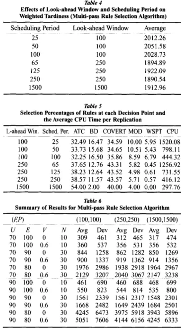
1500 jobs produce the lowest measures without any significant statistical difference between them. The effects of the look-ahead window are listed in Table 4 along with scheduling period levels. It is observed that a look-ahead window set at 250 jobs with scheduling periods of either 65 jobs or 250 jobs produces slightly better performance.

Table 5 shows the selection percentages of each rule along with the average CPU time for one full replication of simulation. The results show that the selection percentages are highly dependent on the lengths of the look-ahead window and scheduling period. Although, ATC and COVERT are more and more selected for longer look-ahead windows, the other rules are alternatively selected in the shorter look-ahead windows. This shows that several rules can be preferred in the short term, although their long-term performances are dominated by others. The table also shows the effects of the look-ahead window and scheduling period on the simulation time. Especially the scheduling period affects the CPU time because it directly determines the frequency of the multi-pass algorithm executions.

A summary of results is provided in Table 6 for selected combinations of look-ahead window (F) and scheduling period (F). It is observed that F = 100 is inferior mainly due to its performance in low efficiency levels. The effect of utilization on the performance of the loo-job look-ahead window is depicted in Figure 7. This figure shows that a sched- uling period of 25 jobs is mostly affected by the utilization. The effects of efficiency and mean down- time are displayed in Figures 8 to 10. In higher effi- ciency levels or in short downtimes, the different

Table 4

Effects of Look-ahead Window and Scheduling Period on Weighted Tardiness (Multi-pass Rule Selection Algorithm) Scheduling Period 2.5 50 100 65 125 2.50 1500 Look-ahead Window .~~ 100 100 100 250 250 250 1500 Average 2012.26 2051.58 2028.73 1894.89 1922.09 1890.54 1912.96 Table 5

Selection Percentages of Rules at each Decision Point and the Average CPU Time per Replication

L-ahead Win. Sched. Per. ATC BD COVERT MOD WSPT CPU 100 25 32.49 16.47 34.59 10.00 5.95 1520.08 100 50 33.73 15.68 34.65 10.51 5.43 798.11 100 100 32.25 16.50 35.86 8.59 6.79 444.32 250 65 37.65 12.76 43.31 5.82 0.45 1256.92 250 125 38.23 12.64 43.52 4.98 0.61 731.55 250 250 38.57 11.57 43.57 5.71 0.57 416.12 1500 1500 54.00 2.00 40.00 4.00 0.00 297.76 Table 6

Summary of Results for Multi-pass Rule Selection Algorithm

uw

C/E V N 70 100 0 10 70 100 0.6 10 70 90 0 30 70 90 0.6 30 70 80 0 30 (100,100) (250,250) (1500,150O) Avg Dev Avg Dev Avg Dev 309 461 312 465 317 474 360 537 356 531 356 532 844 1258 862 1282 850 1269 900 1337 919 1362 914 1356 1976 2986 1938 2918 1964 2967 2129 3207 2040 ?(I67 2147 $238 461 690 460 688 468 699 550 823 544 814 535 800 1561 2339 1561 2317 1548 2301 1668 2482 1649 2439 1684 2501 4245 6473 3975 5918 3943 5896 5051 7606 4144 6156 4245 6333 70 -So -0.6 90 100 b 30~ 10 90 100 0.6 10 90 90 0 30 90 90 0.6 30 90 80 0 30 90 80 0.6 30

look-ahead windows seem to produce very similar performances. This effect becomes stronger when the efficiency is high; however, at low efficiency levels or with long downtimes, longer look-ahead windows yield better performances. In summary, the length of the look-ahead window is effective on the performance, but the scheduling period is not very significant. That is, it is important to select a proper time period for the look-ahead window; if an appropriate look-ahead window is selected then the

scheduling period is not so important. Results of Lead Time Iteration Algorithm

The ANOVA test for the lead time iteration algorithm is presented in Appendix E. The F-test shows

(12)

Journal of Manufacturing Systems Vol. 2a/No. 4 2001 3 3000 e B s 2500 f .E 2000 z 0 1500 G G 1000 500 - 0 70 (LOW) Utilization 90 (High) 500 0

8O%(Low) 90% (Medium) 100% (High) Efficiency

Figure 7

Average Weighted Tardiness vs. Utilization (Multi-pass Rule Selection Algorithm)

Figure 8

Average Weighted Tardiness vs. Effhziency (Multi-pass Rule Selection Algorithm)

7000 1 I z p 5000. S P E 4000- .0, $ & E 2 1 1000. 0 P

Meandu5~tion of breakdown 1OP

Figure 9

J

P

Meanduztionof breakdown 1OP

Figure IO

Average Weighted Tardiness vs. Mean Duration of Breakdown Average Weighted Tardiness vs. Mean Duration of Breakdown (Multi-pass Rule Selection Algorithm, EfBciency=lO%) (Multi-pass Rule Selection Algorithm, Efficiency=90%)

that only the main effects of utilization, variation, efficiency, and downtime are significant. The lengths of the look-ahead window and scheduling period do not have significant impact on the performance of the lead time iteration algorithm. Among the two and higher-level interactions, the interaction between utilization and efficiency and the interaction between utilization and downtime are found significant. The Duncan’s test supports these findings, as shown in Appendix E For the sake of brevity, a summary table for LTI is provided (see Table 7).

There is no significant difference among the performances of the selected combinations of P and P.

One can choose shorter look-ahead windows with equal scheduling periods to save computational effort. From the same table, the effects of utilization,

4000 3500

-

efficiency, and variation levels are observed. When compared with the single-pass algorithms, the multi-pass rule selection algorithm provides 7.5% improvement on average over the single-pass rules. When the utilization is high or the processing time variation is low, multi-pass rule selection algorithm is even more advantageous. The lead time iteration algorithm produces lower weighted tardiness with an average improvement of 9.6% over the single-pass rules. When the LTI algorithm is compared with the multi-pass rule selection algorithm, it is seen that, on average, LTI dominates the latter; however, the improvement rate over the rule selection algorithm changes with respect to the efficiency and processing time variation. Even in these cases, however, the improvement does not seem to be signifi-

(13)

Journal of Manufacturing Systems

Vol. 20/No. 4 2001

Table 7

Summary of Results for Lead Time Iteration Algorithm

(lOO, lOO) i

~ U - - E ~ V - - ~ N ~ A v g - - D e v [ 70 100 0 10 ] 300 448 70 100 0.6 1 0 ' 348 520 70 9 0 30 839 1250 70 70 70 90 90 90 90 90 90 90 0.6 30 80 0 30 80 0.6 30 lOO 6 1 0 100 0.6 1 0 90 0 301 90 0.6 301 80 0 3 0 80 0.6 3 0 941 1409 1956 2952 2073 3121 443 662 i 532 797 i 1506 2241 1682 24891 4096 6184 _i 4293 6412, I (250,250) 1(1500,1500) Avg Dev!' Avg Dev 299 447 307 459 344 514 345 516 838 1251 855 1278 910 13511 911 1354 2005 3032! 2001 3014 2114 3180 2119 3182 442 662' 4 5 2 - 6 7 6 530 792 1 ! 537 803 1548 2323 ' 1576 2358 1738 2596[ 1731 2575 4O85 6161[ 4050 6052 I 4237 6317 i 4356 6498 I

cant especially if the high variability due to processing time variations and machine failures is considered. Hence, either can be implemented in the outlined iterative simulation-based mechanism.

The results of summary tables for alternative schemes are simultaneously analyzed (single-pass, multi-pass rule selection, lead time iteration, see

Tables 3, 6, and 7). The differences observable over

all observations may not be consistent with the more direct comparison of the best single-pass rule (say, ATC) and the best setting for multi-pass algorithms (F -- 250, P = 250). Although both multi-pass algorithms improve performance over single-pass rules on average, this is questionable if it is compared with the best among the single-pass rules, especially in low efficiency levels and high processing time variation levels. This implies that multi-pass algorithms may not pay off the computational effort if the best rule to implement in the system is known. These results also show that a simulation-based scheduling mechanism is effective in more deterministic situations (E = 100 and V = 0). This can be attributed to the nature of the iterative algorithms because they search through the promising improve- ments over the existing alternatives; however, this positive effect of the search ability reduces in the dynamic and stochastic environment (that is, processing time variations and machine breakdowns seriously diminish the potential improvement expected from the iterative algorithms).

Discussion and Conclusions

This study has defined a scheduling environment where some information about future job arrivals (job release data) is available. A simulation-based

scheduling mechanism is outlined. Two types of scheduling decisions were tested for effectiveness: (1) best-rule selection and (2) parameter tuning. Using the multi-pass rule selection algorithm for the first type and the lead time iteration method for the second, an extensive experimental study was conducted by creating both deterministic and stochastic environments (dynamic, however, in all cases). The effects of unexpected events such as machine failures and processing time variation were investigated. The experimental results repeatedly show the significant interactions among the method-specific factors and the system conditions, which supports the first conjecture.

The priority rule is selected to implement during the next scheduling period in the rule selection algorithm, whereas improved waiting time estimates were sought in the lead time iteration method. Namely, higher-level policies are decided at the beginning of a scheduling period, and the selected policies are implemented dynamically over time. The remaining scheduling decisions such as determining the start times of operations (or which job to start next) are determined in a dynamic manner during the implementation of the selected policies (a static a priori schedule is not actually generated, as opposed to the traditional approaches). When unexpected events occur in the system, the dynamic nature of these algorithms results in decisions that are state-dependent as the system state changes. Hence, the algorithms that are dynamic and state- dependent in nature inherently develop their reac- tions to the events until the next decision point. In this sense, the results support our second conjecture that frequent updates of the higher-level policies (short scheduling periods) may not be necessary even in dynamic and stochastic conditions. This observation is especially true when the lead time iteration method is considered. If the algorithm implemented in ISM were not dynamic and robust, then the revision of the policies would be critical.

In this case, the information for the next forecast horizon is utilized explicitly during the decision making process. It is assumed that the arrival times and other characteristics of the jobs are known with certainty at the beginning of scheduling period. The only stochastic events are machine failures and processing time variations; however, the results of the experiments have indicated that these two events do not necessitate frequent revision of the higher-level

(14)

Journal of~anu~ctur~ng Systems Vol. 2oINo. 4 2001

policies. It is expected that if there are order cancel- lations, rush job arrivals, or operational changes in jobs, more frequent scheduling revisions with short-

er scheduling periods would potentially improve the performance. This is left as a future study.

The results also show that the multi-pass or iterative algorithm is better than single-pass algorithms (rules) on average, but not better than the best single-pass rule, especially in stochastic cases. This implies that one may just choose the overall best rule and not need to revise this decision for the entire horizon. This can be explained by the dynamic and state-dependent nature of the rules implemented in the study. Even if the rules are single-pass, they use the up-to-date information about shop status because they defer scheduling decisions until when they are needed. Hence, the rules have inherent adaptive/reactive elements such as changing the priorities of jobs, which make them rather robust for uncertain conditions. Additionally, the results show that fine tuning a parameter of a rule in a series of iterative simulations may not be a viable approach in a stochastic environment. The stochastic events may make the fine-tuned rule/parameter an inferior decision for the implementation; that is, the pe~orm~ce of the rule/parameter that performed best under deterministic conditions may turn out to be a poor selection under stochastic events. These observations provide evidence that support the third conjecture listed previously; however, a further investigation is needed for other types of decisions that would be made by means of iterative simulation and for other types of stochastic events.

References

Aytug, H.; Bha~cha~a, S.; Koehfer, G.J.; and Snowdon, J.L. (1994). “A review of machine learning in scheduling.” IEEE Trans. on Engg. Mgmt. (~41, n2), pp165-171.

Aytug, H.; Koehler, G.J.; and Snowdon, J.L. (1994). “Genetic learning of dynamic scheduling within a simulation environment.” Computers and

Operations Research (~21, n8), pp909-925.

Baker, K.R. and &net, J.J. (1983). “Job shop scheduling with modified due dates.” Journal of Operations Mgmt. (~4, nl), ppl l-22.

Carrel, D.C. (1965). “Heuristic sequencing ofjobs with single and multiple components.” Cambridge, MA: Sloan School of Mgmt., Massachusetts Institute of Technology.

Cho, H. and Wysk, R.A. (1993). “A robust adaptive scheduler for an intelligent workstation controller.” ht ‘1 Journal of Production Research (~3 1, n4), ~~771-789.

Church, L.K. and Uzsoy, R. (1992). “Analysis of periodic and event-driven ~s~heduling policies in dynamic shops.” Znt4 JoumaZ of Computer

Znfegrated Mfg. (v.5, n3), ~~153-163.

Davis, W.J. and Jones, A.T. (1988). “A real-time production scheduler for a stochastic manufacturing environment.” Int? Journal of Computer

Integrated Mfg. (vl, n2), pplOl-112.

Harmonosky, C.M. (1990). “Implementation issues using simulation for

real-time scheduling, control, and monitoring.” Proc. of Winter Simulation Conf., 1990.

Harmonosky, C.M. (1993). “Analysis of two key issues for using simulation for real-time production control.” Proc. of 2nd Industrial Engg. Research Conf., 1993.

Harmonosky, C.M. and Robohn, SF. (1991). “Real-time scheduling in a computer integrated manufacturing: a review of recent research.” Znt?

Journal of Computer Integrated Mfg. (~4, n6), pp33 l-340.

Harmonosky, C.M. and Robohn, SF. (1995). “Investigating the application potential of simulation to real-time control decisions.” Int4 Journai of

Computer Znte~ted Mfg. (~8, n2), ~~126-132.

fshii, N. and Taiavage, J.J. (1991). “A ~nsient-based real-time scheduling algorithm in FMS.” Znt ‘Z Journal ofProduction Research (~29, nl2),

~~2501-2520,

Ishii, N. and Talavage, J.J. (1994). “A mixed dispatching rule approach in FMS scheduling.” Znt ‘1 Journal of Flexible Mfg. Systems (~2, n6), pp69-

87.

Kim, M.H. and Kim, Y. (i 994). ~‘Simuiation-bled real-time scheduling in a Bexible m~ufac~ng system.” Journal of Manu~c~ring @stems (v13, tl2), pp85-93.

Kiran, A.S.; Alptekin, S.; and Kaplan, A.C. (1991). “Tardiness heuristic for scheduling flexible manufacturing systems.” Production Planning and

Control (~2, n3), pp228-241.

Kutanoglu, E. and Sabuncuoglu, 1. (1999). “An analysis of heuristics in a dynamic job shop with weighted tardiness objectives.” Znt ‘Z Journal of P~duction Research (~37, nl), pp165- 187.

Law, A.M. and Kelton, W.D. (1991). SimuZatjon Modeling and Analysis.

New York: McGraw Hill.

Lawrence, S.R. and Sewell, E.C. (1997). “Heuristic, optimal, static, and dynamic schedules when processing times are uncertain.” Journal of

Operations Mgmt. (vl5), ~~71-82.

Manivannan, S. and Banks, J. (1992). “Design of a knowledge-based on- line simulation system to control a rn~ufac~~ng shop floor.” ZIE

Tmns. (~24, n3), ~~72-80.

Morton, T.E. and Pentico, D. (1993). Heuristic Scheduhng Systems with

Applications to Production and Project Management. New York: John

Wiley & Sons.

Ovacik, I.M. and Uzsoy, R. (1994). “Rolling horizon algorithms for a single-machine dynamic scheduling problem with sequence-dependent setup times.” Znt ‘Z Journal of Production Research (~32, n6), pp1243-

1263.

SAS Institute. (1994). “SAS/STAT(R) User’s Guide.” North Carolina: SAS Institute.

Tayanithi, l?; Manivannan, S.; and Banks, J. (1993a). ‘A knowledge-based simulation architecture to analyze interruptions in a flexible manufac- turing system.” Journal of Manufacturing Systems (~11, n3), ppl95- 214.

Tayanithi, I!; M~iv~n~, S.; and Banks, J. (1993b). “Complexity reduction during inte~ption analysis in a flexible manufac~ng system using a knowledge-based on-line simulation.” Journal of Manufacturing Systems (~12, nZ), ~~153-169.

Vepsalainen, A.P.J. and Morton, TX. (1987). “Priority rules for job shops with weighted tardiness costs.” Mgmt. Science (~33, n8), pplO35-1047. Vepsalainen, A.I?J. and Morton, T.E. (1988). “Improving local priority rules with global lead-time estimates: a simulation study.” Journal of hZfg.

and Ope~t~ons Mgmt. (v 1, x12), pplO2- 118.

Wu, S.D. and Wysk, R.A. (1988). “Multi-pass expert control system--a controlischeduling structure for flexible manufacturing cells.” Journat

of Manufacturing Systems (~7, n2), pplO7-120.

Wu, SD. and Wysk, R.A. (1989). “An application of discrete-event simulation to on-line control and scheduling in flexible manufacturing.” Int?

Journal ofProduction Research (~27, n9), pp1603-1623.

Authors’ Biographies

Erhan Kutanoglu is an assistant professor in the Dept. of Industrial Engineering at the University of Arkansas. Before his current position, he has worked as an operations research analyst and development engineer at

(15)

Journal of Manufacturing Systems Vol. 2a/No. 4

2001

IBM Global Services. He received his PhD in industrial engineering from Lehigh University in 1999 and his MS and BS degrees from Bilkent University, Ankara, Turkey. His current research interests include models and algorithms for distributed decision making, game theoretic approaches to combinatorial problems, and robustness under uncertainty with applications to scheduling, logistics, and supply chain management problems. He has published his work in journals such as IZE Transactions and the International Journal of Production Research. He is currently involved in funded projects on truck and driver scheduling problems, interactions of e- commerce transactions and transportation flows, and multi-echelon inven- tory stocking and logistics network design problems. He is a member of IIE and INFORMS.

Ihsan Sabuncuoglu is an associate professor of industrial engineering at Bilkent University, Ankara, Turkey. He received his BS and MS degrees in industrial engineering from Middle East Technical University and his PhD degree in industrial engineering from Wichita State University. Dr. Sabuncuoglu teaches and conducts research in the areas of scheduling, production management, simulation, and manufacturing systems. He has published papers in Simulation, IIE Transactions, Decision Sciences, Internarional Journal of Production Research, International Journal of Flexible Manufacturing Systems, International Journal of Computer Integrated Manufacturing, European Journal of Operations Research, Production Planning and Control, Journal of Operational Research Sociery, Computers and Operations Research, Computers and Industrial Engineering, OMEGA, and Journal of Intelligent Manufacturing. He is on the editorial board of the International Journal of Operations and Quantitative Management and the Journal of Operations Management. He is an associate member of Institute of Industrial Engineers, Institute of Simulation, and Institute for Operations Research and Management Science.

Appendix A

Analysis of Variance for Weighted Tardiness (WT) (Single-pass Rules) Source Model B Error Source R U R*U V R*V u*v R*U*V E R*E U*E R*U*E V*E R*V*E U*V*E R*U*V*E D(E) R*D(E) U*D(E) R*U*D(E) V*D(E) R*V*D(E) U*V*D(E)

DF Sum of Squares F Value 148 4305218750.23 141.46 9 78459689.45 42.40 1251 257243013.65 DF ANOVA SS 4 176377062.06 4 4 4 2 8 2 8 2 8 2 8 4 16 4 16 4 16 4 R*U*V*D(E) 16 1063808.71 729224603.36 66292561.20 6162597.3 1 217221.97 500191.15 130987.23 1841908686.72 88237797.50 275704820.80 33849156.53 858029.21 322360.01 31222.69 262709.14 916468601.08 18004682.52 66818835.40 2886616.38 282567.87 924265.08 229676.86 Pr_gt_F 0.0001 0.0001 F Value _PIXL!? 214.44 0.000 1 3546.30 0.0001 80.60 0.000 1 29.97 0.0001 0.26 0.9011 2.43 0.1191 0.16 0.9588 4478.70 0.0001 53.64 0.000 1 670.39 0.000 1 20.58 0.0001 2.09 0.1246 0.20 0.9915 0.08 0.9269 0.16 0.9958 1114.22 0.0001 5.47 0.000 1 81.24 0.0001 0.88 0.5959 0.34 0.8486 0.28 0.9977 0.28 0.8915 0.32 0.9947

Appendix B

Duncan’s Multiple Range Test for Weighted Tardiness (Single-pass Rules)

Factor: Rules (R) -

Duncan Grouping _.~~ Mean N R

A ~ 2810.84-- 280 ~~~ MOD CB 1911.66 1999.84 2809 280 WSPT ATC C 1907.01 280 BD C Factor: Utilizatiofl Duncan Grouuine 1895.07 280 COVERT

Mean ?-Y Utilization

1

~._.

i

2826.60

B 1383.16

Factor: Processing Time Variation (V)

Duncan Grouping Mean

A 2171.23 700 90 700 70 N Variation 700 0.6 B 2038.53 700 0

Factor: Efficiency (E)

Duncan Grouping _{~____.}Mean N Efficiency

A 3383.75 600 80

B 1373.59 600 90

C 462.12 200 100

Appendix C

Analysis of Variance for Weighted Tardiness (WT) (Multi-pass Rule Selection Algorithm)

Source DF Sum of Squares F Value Pr gt F

Model 204 5336807534.54 93.04 0.000 1 B Error Source U 175: DF 1 V 1 u*v 1 E 2 U*E 2 V*E 2 U*V*E 2 D(E) U*D(E) t V*D(E) 4 U*V*D(E) _\I 4 F 2 “,:; 2 ₂ U*V*F 2 g’,*F 4 V*E*F t U*V*E*F 4 D*F(E) U*D*F(E) : V*D*F(E) 8 ;;F;*Diti(E) 8 4 U*P(F) 4 V*P(F\ 4 U*E*P(F) ! V*E*P(F) ;:J(;yFP)(F) : U*D*P(E*F) :: V*D*P(E*F) 16 U*V*D*P(F) 16 128727548.77 493474510.01 ANOVA SS ___._ 857480788.75 9672458.36 995615.25 2353820883.82 370356964.26 1462751.85 178918.97 1362144691.42 146419209.21 1236815.98 1863158.63 7611557.59 7214977.51 98048.79 16597.43 11283954.31 9492677.70 153526.66 42890.62 12603550.76 10231745.42 1458950.07 1014110.52 382086.21 363088.62 1105326.33 1151821.94 250406.36 529866.13 1950854.5 1 1587157.07 9353208.53 9186562.31 7835016.21 7529747.64 50.87 0.0001 F Value Pr gt F 3049.56 0.0001 34.40 0.0001 3.54 0.0600 4185.58 0.0001 658.57 0.0001 2.60 0.0745 0.32 0.7275 1211.09 0.0001 130.18 0.0001 1.10 0.3551 1.66 0.1575 13.53 0.000 1 12.83 0.0001 0.17 0.8400 0.03 0.9709 10.03 0.000 1 8.44 0.0001 0.14 0.9688 0.04 0.9972 5.60 0.0001 4.55 0.0001 0.65 0.737 1 0.45 0.8906 0.34 0.8513 0.32 0.8628 0.98 0.4157 1.02 0.3934 0.1 I 0.9988 0.24 0.9843 0.87 0.5435 0.71 0.6869 2.08 0.0072 2.04 0.0086 1.74 0.0338 1.67 0.0452