A New approach in the maximum flow problem

!.. NSW A r

-ІЮ

СН Ш

xÆsrZTTUM ZLO ѵУ РііОЖЯМ

_{:: TF EOGI}

_TS^

_{NQ Í.ND SCIB}

_TC

O -Z -.iT U i:b7FîlS!T Y

.„..3 Ν Ί' OF Ί'Η Β O F O U îR E M E iW

A NEW APPROACH IN THE MAXIMUM FLOW PROBLEM

A THESIS

SUBMITTED TO THE DEPARTMENT OF INDUSTRIAL ENGINEERING

AND THE INSTITUTE OF ENGINEERING AND SCIENCES OF BILKENT UNIVER SITY

IN PARTIAL FULFILLMENT OF THE REQUIREMENT FOR THE DEGREE OF

MASTER OF SCIENCE By Aysen Eren July, 1989

A

tarafiadan balij^laonustir.

T •5>.S5

E r ZS

I certify that I have read this thesis and that in my opinion it is fully a dequate,in scope and in quality, as a thesis for the degree of Master of Science.

Assoc. Prof. M u s t a f a Akgiil (Principal Advisor)

I certify that I have read this thesis and that in my opinion it is fully adequate,in scope and in quality, as a thesis for the degree of Master of Science.

Assoc. Prof. Omer Kirca

I certify that I have read this thesis and that in my opinion it is fully adequate,in scope and in quality, as a thesis for the degree of Master of Science.

A s s o c . f. Osman Oguz

I certify that I have read this thesis and that in my opinion it is fully adequate,in scope and in quality, as a thesis for the degree of Master of Science.

Asst. Prof. Barbaros Tansel

Approved for the Institute of Engineering and Sciences

Prof. Mehmet Bari

Director of Institute of Engineering and Sciences

ABSTRACT

A NEW APPROACH IN THE MAXIMUM FLOW PROBLEM

A Y S E N EREN

M.S. in Industrial Engineering Supervisor: Assoc. Prof. Mustafa Akgul

July, 1989

In this study, we tried to approach the maximum flow problem from a different point of view. This effort has led us to the development of a new maximum flow algorithm. The a lgorithm is based on the idea that when initial quasi-flow on each edge of the graph is equated to the upper capacity of the edge, it violates node balance equations, while satisfying capacity and non-ne gativ it y constraints. In order to obtain a feasible and optimum flow, quasi-flow on some of the edges have to be reduced. Given an initial quasi-flow, positive and negative excess, and, balanced nodes are determined. A lgorithm reduces excesses of unbalanced nodes to zero by finding residual paths joining positive excess nodes to negative excess nodes and sending excesses along these paths. M inimum cut is determined first, and then ma x i m u m flow of the given cut is found. Time complexity of the algorithm is o(n^m). The application of the modified version of the Dynamic Tree structure of Sleator and Tarjan reduces it to o(nmlogn).

Ö Z E T

MAKSİMUM AKIŞI EKO B L E M± NTE

YENİ BİR YAKLAŞIM A y ş e n Er en E n d ü s t r i M ü h e n d i s l i ğ i B ö l ü m ü Y ü k s e k L i s a n s Tez Y ö n e t i c i s i : Doç. M u s t a f a A k g ü l Temmuz, 1989 Bu ç a l ı ş m a d a , m a k s i m u m akış p r o b l e m i n e d e ğ i ş i k b i r gö rü ş n o k t a s ı n d a n y a k l a ş m a y ı de n e d i k . Bu uğraş, bizi yeni b i r m a k s i m u m akış a l g o r i t m a s ı n ı g e l i ş t i r m e y e gö t ü r d ü . A l g o r i t m a , s e r i m i n he r a y r ı t ı n d a k i ilk a k ı ş ı m s ı n ı n , a y r ı t ı n üst k a p a s i t e s i n e e ş i t l e n d i ğ i zaman, b u n u n k a p a s i t e ile eksi o l m a m a k ı s ı t l a r ı n ı sa ğl ar ke n, d ü ğ ü m d e n g e e ş i t l i k l e r i n i b o z m a s ı fikr in i te me l alır. O l u r l u ve en iyi b i r akış e l d e e t m e k için, bazı a y r ı t l a r ü z e r i n d e k i a k ı ş ı m s ı l a r a z a l t ı l m a l ı d ı r . V e r i l e n b i r ilk a k ı ş ı m s ı y a göre, artı ve eksi f a z l a l ı k ile d e n g e l e n m i ş d ü ğ ü m l e r b e l i r l e n i r . A l g o r i t m a , ar tı f a z l a l ı k d ü ğ ü m l e r i n i eksi f a z l a l ı k d ü ğ ü m l e r i n e b a ğ l a y a n a r t ı k y o l l a r ı n ı bu lup, bu y o l l a r b o y u n c a f a z l a l ı k l a r ı g ö n d e r e r e k , d e n g e l e n m e m i ş o l a n d ü ğ ü m l e r i n f a z l a l ı k l a r ı n ı s ı f ı r a indirir. İlk önce, en k ü ç ü k k e s i t b e l i r l e n i r ve s o n r a v e r i l e n k e s i t i n m a k s i m u m ak ış ı b u l u n u r . A l g o r i t m a n ı n z a m a n s a l k a r m a ş ı k l ı ğ ı 0 ( n 2 m ) ’dir. S l e a t o r ile T a r j a n ’ın D i n a m i k A ğ a ç y a p ı s ı n ı n d e ğ i ş t i r i l m i ş ş e k l i n i n u y g u l a n m a s ı b u n u 0 ( n m l o g n ) ' e d ü ş ü rü r. 1 V

ACKNOWLEDGEMENT

I would like to thank to Assoc. Prof. Mu stafa Akgül for his supervision, guidance, valuable suggestions , comments, and patience throughout the development of this thesis,

I am grateful to the members of Jury: Assoc. Prof. Ömer Kirca, Assoc. Prof. Osman Oguz, and Asst. Prof. Barbaros Tansel for their valuable comments.

My sincere thanks are due to Levent Aksoy for giving me his morale support to complete this study, and for his great help in correcting and printing my thesis.

TABLE OF CONTENTS

Introduction and Literature Review Definitions and Notation

Conceptual Description of the Al gorithm The M a ximum Flow A l g o rithm

i . The Fi rst Stage i i . The Second Stage

iii. A Formal Version of the Algo rithm

iv. An A p p l i cation of the Proposed Alg orithm

V. An A l te r native Procedure for the Second Stage

The Dynamic Tree Version of the Algorithm Conclusions and Future Research

References 1 10 15

21

21

VI

LIST OF FIGURES

m · "I · Node sets of G and residual edges connecting them 17 at the end of the first stage.

‘ II

II I . 2. The subgraphs of G . 13

I V . iv.1. A sample network g. 3 5

IV.iv.2. Graph G . 3 3

IV.iv.3. Initial search tree. 33

IV.iv.4. Search tree at the end of first stage. 3 7

— J

IV.iv.5. (S,S) cut on G . 3 7

IV.iv.6. Search tree at the beginning of second stage. 38

IV.iv.7. Final flows on the edges of G. 38

II

C H A P T E R I

INTRODUCTION AND LITERATURE REVIEW

The problem of finding a ma xim um flow in a directed graph with edge capacities has interested many people in various fields. It is a w e l l-defined problem and has been known for many years. Its applications cover a wide area extending from mi nimum cost flow problems to the analysis of transmission networks.

The problem can be stated and formulated as a Linear Program. Given a directed graph, with capacities on the edges and two distinct nodes, a source s and a sink t, the m a ximum flow problem is to maximize the flow that can be sent from source to sink through the network. A flow is an assignment of real numbers to edges of the graph which sati s f у ;

i. capacity constraints which make sure that flow on each edge is always smaller than or equal to edge capaci t y ,

ii. node balance constraints which state that total flow coming into each node should pass it without any loss or gain in value, and,

iii. n o n-negativity constraints.

Let V be the total flow passing through edges of the network. Let f, u and A denote respectively flow, capacity vectors, and the incidence matrix. Then the LP model of the

ma x i m u m flow problem is; M A X V s . t , A * f = f < u f > 0 - V V

0

The first step toward the esta bli shment of the max-flow m in-cut theorem has been taken by Menger [5,17] in the early thirties. The theorem of Menger states that if source and sink are di sconnected by removing k nodes of the graph, meaning that all paths from source to sink should pass thru at least one of k nodes, there are k source-sink internally disjoint paths on the graph. Originally stated for undirected graphs, it is directly applicable to the theory of max-flow min-cut, when formulated in terms of digraphs.

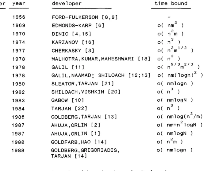
The max-f l o w min-cut theorem has been established by two independent groups of people. Shannon, Feinstein and Elias [7] and Ford-Fulkerson [8] have stated the theorem in 1956. Then the first max-flow algorithm has been developed by Ford-Fulkerson in the same year. In the following years, many fast and e fficient algorithms have appeared in the literature. Table 1 gives these algorithms in chronological order. Time bounds are given in terms of n -number of

nodes, m -number of edges and N -maximum edge capacity.

number year developer time bound

1 1956 FORD-FULKERSON [8,9]

-2 1969 EDMONDS-KARP [6] o( nm )

3 1970 DINIC [4,15] o( n m )2 X

4 1974 KARZANOV [16] o( n )

5 1977 C HERKASKY [3] o( n m 2 1/2 . )

6 1978 MALHOTRA,K U MA R , MAH ESHWA RI [18] o( n 2 X)

5/3 2/3 V

n m )

7 1978 GALIL [11] o(

8 1978 GALIL,NAAMAD; SHILOACH [12;13] o( nm(logn)^ )

9 1980 S L E A T O R , TARJAN [21] o( nmlogn ) 10 1982 S HILOACH,VISHKIN [20] o( n ) 1 1 1983 GABOW [10] o( nmlogN ) 12 1984 TARJAN [22] o( n 3 V) 13 1986 G O L D B E R G , TARJAN [13] o( nmlog(n^/m) 14 1987 AHUJA,ORLIN [2] o( nm+n^logN ) 15 1987 AHUJA,ORLIN [1] o( nmlogN ) 16 1988 G O L D F A R B , H A O [14] o( n m ) 17 1988 G O L D B E R G ,G R I G O R I A D I S , o( nmlogn ) TARJAN [14]

Table 1. Max-flow algorithms in chronological order.

Five of the listed algorithms have great importance and impact on the history of max-flow algorithms. They are F o r d - F u l k e r s o n , Edmonds-Karp, Dinic, Karzanov and Goldb e r g - T a rja n algorithms.

Being the first max-flow algorithm, Ford-Fulkerson algorithm is of importance. The al gorithm starts with any feasible flow and augments or increases the flow by finding a source- t o - s in k directed path in the residual graph. The

algo r i t hm stops when there is no augmenting path. The proof of optimality is given by exhibiting a cut having the capacity that is equal to the given flow. Their algorithm is also known as Labelling algorithm. The Labelling algorithm is a n o n - deterministic algorithm to find a s o u rce-to-sink directed path in the residual graph in which nodes to be scanned are chosen arbitrarily among the labeled nodes. With integral edge capacities, the upper bound on the number of iterations is obviously equal to the value of the flow. Major deficiency of the algorithm is its exponential complexity. When capacities are irrational, the a lgorithm may not even be finite and may converge to a n o n - m aximum flow as exhibited by Ford-Fulkerson [9].

Thirteen years later, Edmonds and Karp [6] employed b readth-first search method to find shortest residual augmenting paths from source to sink. Their algorithm is the first strongly polynomial maximum flow algorithm; it requires o(nm) augmentations and o(nm^) time.

D i n i c ’s a lgorithm [4] works on a layered graph which contains all the shortest paths in the current residual graph. In a layered graph, source and sink are placed in distinct layers by themselves. There are other layers between layers of source and sink. Each edge in such a graph goes from one layer to the next layer. Thus all source-sink paths have the same length and the layered graph is acyclic. In each layered graph one finds a maximal or blocking flow. A blocking flow in a layered graph assures that in the next layered graph, length of any

source-to-si nk path is increased by at least one. Thus there are at most ( n-1 ) layered graphs. By using depth-first search, Dinic finds a blocking flow in o ( nm ) time, giving total bound of o ( n^m ).

D i n i c ’s a lgorithm has been modified by many people leading to the develo p m e n t of more efficient and faster algorithms. Sleator and Tarjan [21] designed a new data structure. Dynamic Tree, particularly for D i n i c ’s algorithm. With Dynamic Trees, SIeator-Tarjan succeeded to reduce the running time of the m a ximum flow algo rithm from o(n^m) to o(nmlogn). In 1987, Ahuja and Orlin [1] modified D i n i c ’s a l gorithm and obtained ( nmlogN ) time bound by using a scaling algorithm and utilizing a distance label function instead of maintaining layered graphs. Their bound is weakly polynamial due to dependence on input parameter N which is the maximum edge capacity. However their algorithm requires no complex data structure. Distance label function has been introduced by Goldberg and Tarjan in 1986

[13]. It is a function from node set to positive integers. Distance label of a node is the minimum length of augmenting path from a reference node to that node.

In 1974, Karzanov [16] introduced his algorithm to find a blocking flow in a layered graph and approached maximum flow p r oblem from a different point of view. Until that time, developed algorithms were based on the idea of augmenting flow on residual paths. Residual paths which go from source to sink are found one by one and as much a flow is sent thru each path as possible. The maximum amount

of flow which can be sent along a path is equal to the mi nimum of residual capacities of edges on that path. When a flow is augmented, it saturates at least one edge. Hence no more flow can be sent along that path. Such a path is called saturated or blocked, and such a flow, a blocking flow. In his algorithm, Karzanov uses the idea of Preflow to determine a blocking flow or a maximal flow of a layered graph. The Preflow concept has been introduced by Karzanov. It is a mapping from the edge set to non-negative real numbers that satisfies two types of inequalities. Let p be a Preflow. Then

p( i,j ) < capacityC i,j ) for all ( i,j ) pairs and

E

> E

The first inequality makes sure that the Preflow does not disturb capacity constraints. The satisfaction of node balance equations is not guaranteed due to the second type of inequalities. Incoming Preflow may be greater than outgoing Preflow at any node. K a r z a n o v ’s algorithm consists of phases. Before each phase starts, a layered graph is constructed, then a Preflow is sent through edges of the graph by pushing as much flow from source toward nodes as possible. Unbalanced nodes or nodes with positive excesses are taken one by one and balanced by reducing flows coming into them. A phase ends when all nodes are balanced and a maximal flow in the layered graph is obtained. D i n i c ’s and

K a r z a n o v ’s algorithms differ in the way they find maximal flows. Time bound of the algorithm is o( n^) and it is the best for dense graphs.

In 1986 , Goldberg and Tarjan used the Preflow idea of Karzanov. They also maintained distance label function and Dynamic Tree structure and reduced the order to o( nmlog(n /m) ). It is the best bound both for sparse and dense graphs so far.

Recently Goldfarb and Hao developed the first strongly polynomial primal simplex algorithm for the maximum flow problem. They obtain the maximum flow in at most o( nm ) flow a ugmentations or simplex pivots. They employed the rule that is to select an edge which is closest to source node among the non-basic edges which are candidates to enter the basis.

Goldberg, Grigoriadis, and Tarjan [14] have obtained o(nmlogn) time bound for G o l d f a r b - H a o ’s primal simplex algorithm by using a modified version of Dynamic Tree data structure of Sleator and Tarjan.

In this study, we approach the classical maximum flow problem from a different point of view and propose a new m a ximum flow algorithm. Our algorithm originates from Goldb e r g - T arja n [13] and feasible distribution algorithms [19]. It is based on the idea that if the flows on edges are assumed to be equal to upper capacities, node balance equations of some nodes will be violated. In order to find an o p timum solution, node balance equations have to be satisfied. Our algo r i t h m does precisely that.

Goldberg and Tarjan uses K a r z a n o v ’s idea of Preflow. We will introduce a quasi-flow concept and use it. Qua s i - f l o w is a special type of flow, satisfying upper capacity and non-negativity constraints on the edges of the graph. In their algorithm, there are positive excess nodes, called active or unbalanced nodes. By reducing flows on paths which connect source to active nodes, all the nodes are balanced. Both positive and negative excess nodes occur due to quasi-flow in our proposed algorithm. Negative excess nodes have opposite properties of positive excess nodes. In order to balance them, we have to find paths from negative excess nodes to positive excess nodes and reduce flow on them. The global framework of the algorithm is very similar to feasible distribution algorithms. Our algorithm makes use of K a r z a n o v ’s Preflow concept and also defines Postflow. There are two inequalities that are required to make a flow Postflow. First one makes sure that the flow on each edge is between zero and upper capacity of that edge. The second inequality states that the flow going out of each node is greater than or equal to flow coming into it. In that sense, the Postflow can be seen as the reverse of the Preflow.

There are 6 chapters including introduction. The Next chapter contains definitions and notation. Conceptual description of the a lgorithm is given in the 3rd Chapter. Chapter 4 consists of the algorithm, proofs showing its polynomiality, correctness, and a sample problem. Dynamic tree version of the algorithm is presented in Chapter 5.

Chapter 6 summarizes the study, findings, and future r e s e a r c h .

C H A P T E R II

DEFINITIONS AND NOTATION

G = (N,E) defines a directed graph with node set N and edge set E. There are two distinct nodes, one called source, the other called sink. We assume that all edges incident to the source are directed away from the source and all edges incident to the sink are directed into the sink. Thus source node behaves like a real source and can only send flow to other nodes while sink can only receive flow. Let s stand for the source node and t for the sink. The lower capacity of each edge is taken to be zero. Edges have finite upper capacities; u(i,j) stands for the upper capacity of edge (i,j). The proposed algorithm utilizes the concept of a quasi-flow. A quasi-flow is a real valued function g, defined from the edge set to real numbers that satisfies the condition

0 < g ( i , j ) < u ( i ,j ) V ( i ,j ) e E.

A quasi-flow does not violate edge capacity constraints, however it may violate node balance equations. Therefore it is not, in general, ^ a feasible flow. Initially, the quasi-flow of every edge is equated to its upper capacity.

It is assumed that one artificial edge ( t,s ) links sink to source. Algorithms , using such an edge, for the sake of simplicity, assume an infinite capacity for it. We, for the sake of the algorithm, assign a finite value to the

capacity of that edge. That value will be defined soon. Excess function, which will be defined next, makes use of the capacity assigned to ( t,s ) in defining excesses of source and sink nodes. During the first stage, the existence of ( t,s ) is ignored. Consequently, excesses of source and sink nodes remain fixed because of non-existence of ( t,s ). The algorithm uses it in the second stage to balance node equations, after finding the m i nimum cut.

The algorithm m a intains two functions. The first one is the excess function e, defined from node set to real numbers. For any node i, excess of i is the difference between total quasi-flow coming into node i and total quasi-flow going out of node i. Let us formalize the concept and define the excess function as follows;

e ( i ) = <

« - Outflow(s) if i = s Inflow(t) - cx if i = t Inflow(i) - Outflow(i) o. w.

where

Inflow(i) : sum of quasi-flows of edges coming into node i on G.

Outflow(i) : sum of quasi-flows of edges going out of node i on G .

a : ( Ile(i)l + max ( u , u,}), where u is the_{»1 8 t 8} V i € N \ < s , t }

total capacity of outgoing edges of s and and u^ is the total capacity of incoming edges of t.

The purpose of using a is to make excess function to take a positive value at source node and a negative value at sink node, and make them connected to supersource and supersink, respectively, throughout the first stage. It will help us to define a cut right after the completion of the first stage. That point will be discussed later. In, order to make e(s) a positive number and e(t) a negative number, a has to be greater than max{ u , u }. _{8 t} Instead of saying that a is any number greater than max{ u , u, }, it is set to be equal to the sum of absolute values of excesses of nodes excluding source and sink and max{ u , u, }.

Two artifical nodes are created and added to graph, a supersink ss and a supersource st node. New node set is N = N u {ss,st}. Supersink is connected to each negative excess node by an artificial edge directed from st to that node. Similarly, artificial edges directed from positive excess nodes to ss are used to connect ss to the graph. Each artificial edge has a capacity that is equal to the excess of the node, to which it is adjacent. Edge set is enlarged by the addition of artificial edges and denoted by

I I <1 I I II

E . The new graph becomes G = ( N , E ). Supersink st becomes a negative excess node whose excess is the sum of negative excesses. Supersource ss has a positive excess that is equal to the sum of positive excesses. In the beginning, except these two, nodes with excesses are temporarily balanced.

II I I M

The a l gorithm works on residual graphs. G^(N ,E^)

indicates residual graph with node set N and residual edge

II

set E^. If there is a quasi-flow on the edge ( i,j ), it results in two residual edges. r(i,j) is the capacity of a forward residual edge directed from i to j and r(j,i) is the capacity of a backward residual edge directed from j to i. r(i,j) and r(j,i) have contrary meanings with respect to edge (i,j). r(i,j) is the additional possible flow increase orl edge (i,j) while r(j,i) is the possible flow decrease on edge (i,j). They are defined symbolically as,

r ( i ,j ) = u ( i ,j ) - g ( i ,j ) r ( j ,i ) = g ( i , j )

A search tree is costructed by breadth-first search on the residual graph. The algorithm maintains it to determine residual paths connecting supersource to supersink. A search tree can be defined as a special type of distance directed branching. Let us first give the definition of a directed branching. It is a tree in which every node, other than root, has exactly one incoming edge. Hence, every path from the root to any other node in a branching is unique. Besides that, in a search tree every unique path is a shortest path in the residual graph. Search tree concept is very similar to the shortest path tree concept used in A h u j a - O r l i n ’s algorithm [1]. The main point that d istinguishes it from our a lgorithm is that a shortest path tree is a spanning tree whereas a search tree does not have to hold all of the nodes. Our search tree is rooted at supersource. While the algorithm proceeds, constructed tree

goes under frequent structural changes. Several tree operations like deletion of edges and addition of new nodes, are carried out to reflect those changes by using distance label function. L e t ’s now introduce the distance label f u n c t i o n .

The Distance Label function is the second function used by our algorithm. It is defined from the node set to non-negative integers and the primary reason for using it is to c o nstruct and update the tree structure which is under frequent change during the execution of the algorithm. Distance label of node i, d(i), is the minimum number of edges that are on the path of the search tree , connecting i to supersource. The function i s valid if it satisfies the following conditions:

i . d( i ) = d( j ) + 1 if r (j , i ) > 0 , (j,i) e T, i i . d ( i ) > d( j ) + 1 if (j,i) e e".

C H A P T E R III

CONCEPTUAL DESCRIPTION OF THE ALGORITHM

Before explaining the algorithm conceptually let us first describe the graph we will work with.

A few additions are made to the original graph G. An artificial edge ( t,s ) with finite lower and upper capacities is assumed to join sink to source. For rotational and algorithmic convenience two dummy nodes, supersource and supersink are introduced and as mentioned

• I

in Chapter II, graph G is formed. Then an initial flow called quasi-flow is assigned to the edges of G . Node excesses are determined and then node set is divided into three disjoint subsets: set of positive excess nodes N(+), set of negative excess nodes N(-) and set of balanced nodes N(O). The excesses of the nodes have to be zeroed to obtain a feasible and o p timum flow on the graph. Accordingly, the problem definition is modified slightly and classical maximum flow problem becomes problem of sending positive excess of supersource to supersink through residual graph or equiva l e n t ly sending positive excesses of nodes of N(+) to nodes of N(-) along residual paths.

The structure of the a lgorithm is quite similar to the feasible distribution algorithm applied to the maximum flow problem. That is investigated in detail by Rockafeller [19]. Before giving evidence for the equivalence of our a lgorithm and the feasible distribution algorithm, let us first define the feasible distribution algorithm. It is

stated as follows: Given the capacity bounds on edges, the supply value of each node is determined by subtracting its inflow from its outflow. Let b(i) be the supply value of node i. Positivity of b(i) indicates that node i behaves like a supply node and sends some amount of flow. Feasible distribution problem is to find a flow f, such that f conserves capacity constraints of the edges and also satisfies supply constraints. The conceptual algorithm designed to solve the feasible distribution problem is modified and applied to the maximum flow problem. In that case, an initial flow x, which satisfies edge capacity c onstraints is given. Looking at x, supply values or in our words excess values ( b(i) = - e(i) ) of nodes are determined and, N(+) and N(-) are defined. If two sets are empty, initial flow x is feasible and optimal, otherwise excesses of nodes should be zeroed. The painted network a lgorithm [19] that employes a graph search in a suitably constructed residual graph is applied to reduce excesses to zero.

Our approach is similar to the one discussed above. In the above case, there is no restriction on the initial flow, we assume that the initial quasi-flow on each edge is equal to its upper capacity. Instead of using the painted network algorithm, we propose our a lgorithm which is easier to understand and manipulate. For convenience and easiness in defining a mi nimum cut set, instead of applying the algorithm to residual graph of G once, we repeat our a lgorithm twice.

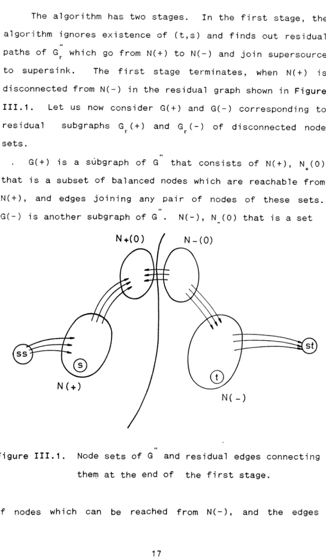
The algorithm has two stages. In the first stage, the algorithm ignores existence of (t,s) and finds out residual paths of which go from N(+) to N(-) and join supersource to supersink. The first stage terminates, when N(+) is disconnected from N(-) in the residual graph shown in Figure III.1. Let us now consider G( + ) and G(-) corresponding to residual subgraphs G ( + ) and G (-) of disconnected node_{r r} s e t s .

, G( + ) is a subgraph of G that consists of N( + ), N^(O) that is a subset of balanced nodes which are reachable from N( + ), and edges joining any pair of nodes of these sets. G(-) is another subgraph of G . N(-), N (0) that is a set

Figure III.1. Node sets of G and residual edges connecting them at the end of the first stage.

of nodes which can be reached from N(-), and the edges

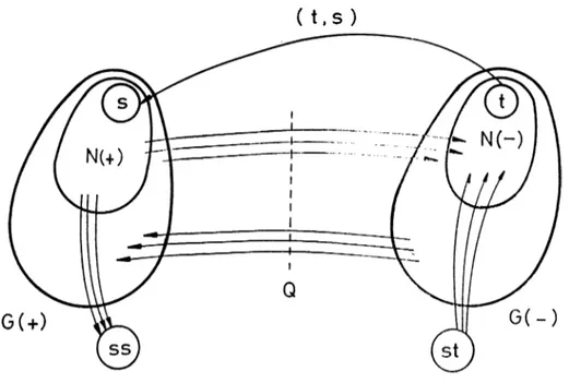
connecting nodes of these sets belong to this subgraph. G(+) and G(-) are connected by an artificial edge (t,s) and a set of edges Q, which consists of the the edges between these s u b g r a p h s .See Figure III.2. Let us now investigate the flows on G( + ) and G(-), and derive some interesting r e s u l t s .

The quasi-flow on edges of G( + ) can be redefined as a Pheflow. It satisfies the conditions required to make a flow a Preflow. Q ua s i-flow on each edge is between zero and given upper bound and inflow of each node of G(+) is greater than or equal to its outflow.

Let us now investigate the other subgraph G(-). We call the quasi-flow on G(-) Postflow. It satisfies capacity constraints of edges of G(-) and outflow of each node is greater than or equal to its inflow.

( t.s )

Figure III.2 The subraphs of G

We must somehow manipulate Preflow and Postflow on edges of G( + ) and G(-) such that excesses are reduced to zero. In G(+), source node sends flow to other nodes, hence all positive excess nodes are connected to source by paths that carry Preflow. These paths correspond to residual paths going from nodes of N(+) to source. Balancing a positive node means to push its excess toward source along the residual path.

Similarly, sink absorbs Postflow coming from nodes of N(-). Negative excess nodes are connected to sink by means of paths which carry Postflow. These paths correspond to residual paths which are directed from sink to nodes of N(-). In order to send negative excess of any node to sink, we either reduce flow on paths that carry Postflow or send flow through residual paths that reach that node. We will prefer to use residual paths for the stability of the a l gorithm and make use of search tree that is on hand at the end of the first stage.

Goldberg and T a r j a n ’s Reduce/Relabel step [13] could be modified and extended to take care of both negative and positive nodes and applied to the problem as well. This alternative procedure will be discussed in the next chapter.

In the second stage, instead of reducing excesses of G ( + ) and G (-) graphs independently, we connect them by_{r r} residual of ( t,s ). The procedure of the first stage is applied to the new residual graph. Positive excesses are pushed toward negative excess nodes along residual paths which pass thru ( s,t ) edge.

The details about the algorithm, its stages, the procedure used to carry out balancing operation and related results will be given in the next chapter.

C H A P T E R IV

THE MAXIMUM FLOW ALGORITHM

The algorithm determines the max-flow of a network in two stages. The task of the first stage is to get a min-cut set and that of the second stage is to obtain the c orresponding max-flow. The point that distinguishes it from many other well-known algorithms is that instead of finding a max-flow first and then defining a min-cut set , algo r i t hm first defines min-cut set and then finds max-flow. In this respect, it is similar to Goldberg-Tarjan [13]. The a lgorithm approaches an optimum solution from dual side of the model. The first stage provides dual optimum solution of the problem. When the first stage ends, some nodes may remain unbalanced and consequently the problem may still be primal infeasible. During the progress of the second stage, the a lgorithm approaches a primal op timum solution of the dual optimum. In this chapter, the first two stages of the algorithm will be described. Later on, the convergence of the a lgorithm toward the optimum will be shown to take a polynomial number of steps, and a sample problem will be given.

i . THE FIRST STAGE

Initially edge flows are set to be equal to upper capacities and excesses of nodes are determined. Two dummy nodes, namely, supersink and supersource are created and

added to node set N . Positive excess nodes are connected by forward artificial edges to supersource each having a capacity that is equal to the excess of the node it is coming out of. In a similar way, artificial edges directed to negative excess nodes are used to connect supersink to these nodes. Since source has a positive excess , it is also connected to supersource. Meanwhile sink with a negative excess is adjacent to an artificial edge coming

M

from supersink. New graph G with dummy nodes and artificial edges is constructed. Next step is to find the initial distance labels of nodes. Distance label of supersource is zero and it remains as zero throughout the progress of the algorithm. Starting from supersource, initial distance labels of nodes are determined by

II

breadth-first search on G _r which takes o(m) time. The initial search tree is constructed by using these distance labels of nodes. Therefore the resulting tree is a shortest path tree of the residual graph.

In the first stage, source and sink nodes are treated as distinct nodes and they are connected to dummy nodes depending on their excesses. The algorithm basically searches for shortest residual paths, starting from supersource and ending up at supersink by making use of the distance label function. These residual paths can be called flow-augmenting paths, since once such a path is found,, as much flow is sent through it as possible. From this aspect, the a lgorithm can be considered to be a flow-augmenting algorithm.

The distance label of supersink k gives the lengths of the flow-augmenting paths. Similarities between Edmonds-Karp and this algorithm, and, between D i n i c ’s and this a lgorithm can be seen at the first sight. Like Edmonds-Karp algorithm, it searches shortest paths by breadth-first search and like D i n i c ’s algorithm the search continues until all paths of length k are found. When there remains no path of length k, meaning that it is required to increase the distance label of supersink, its distance label is updated and it becomes 7. The algorithm guarantees that 7 is strictly greater than k. Then the a lgorithm proceeds by searching new augmenting paths of length 7. At this point, phase concept can be brought into the picture. A phase finds flow-augmenting paths of a given length, which is the distance label of s u p e r s ! n k ,and sending flow from ss to S t along them. The main advantage of using the phase concept is to differentiate lengths of augmenting paths and search them in ascending order of their lengths and therefore give a concrete structure to path-searching process.

In any phase, the algorithm proceeds by maintaining a search tree rooted at s upersource and pushing flow along residual paths of length k, connecting ss to st. Whenever a path is determined, flow is sent thru. The amount of flow, denoted by A , is the minimum of residual capacities of edges on the path. Flow is sent and residual capacites of edges are updated. A is either residual capacity of any one of artificial edges or residual of an

original edge of the graph. Depending on whether residual edge is artificial or not, two cases occur;

I. Saturation of the artificial residual edges.

There are two artificial edges on the path. If the one which is adjacent to supersource is saturated, then the corresponding positive excess node is balanced . If the other one, adjacent to supersink, is saturated, then a negative excess node is balanced. Once any artificial residual edge is saturated and deleted from the graph, it is never added to subsequent search tree. Push is said to be excess zeroing.

II. Saturation of any edge.

If A equals m i nimum residual capacity of an original edge on the path, then push is said to be excess non-zeroing. In other words, a unique path of the tree is blocked. No more flow could be sent through it. Since the residual capacity of an edge is used up, a part of the tree which consists of that edge and its successors are disconnected from the search tree. They are temporarily deleted from search tree.

In the case of ties, the one which is closest to supersource is processed first.

Tree is updated to reflect changes in the tree structure. Let ( i,j ) be the edge that is saturated and deleted from the tree. Edges going into node j are examined. If an edge ( k,j ) satisfying conditions of d(j) = d(k) + 1 and r(k,j) >0 is found, no relabeling takes

place. It is called a replacement. New edge ( k,j ) is added to the tree. If not, node j is relabeled and its distance label becomes,

d(j) = min { d(i) + 1 I r(i,j) > 0 and i e T }

Deletion of edge (i,j) disconnects a sub-tree from the search tree. Node j becomes the root of that sub-tree. If the sub-tree has more than one node, it indicates that distance labels of nodes of sub-tree have been determined according to d(j). Hence after updating the distance label of node j, distance labels of nodes of sub-tree should be revised. Nodes are placed in a first come last serve stack according to decreasing order of their distance labels so that node with smallest distance label is at the top. Until stack becomes empty, following procedure is repeated. Node, say z, is taken from top of the stack and its distance label

is updated according to

d(z) = min { d(i) + 1 I r(i,z) > 0 }.

The following Lemma shows that relabeling does not violate validity of distance labels of nodes.

Lemma I V . 1: In every phase a valid search tree of shortest paths is constructed.

Proof: The initial tree is a valid search tree. During execution, the tree is grown, new augmenting paths

are found and excess zeroing or non-zeroing pushes are made. The tree grows while keeping validity conditions of the search tree satisfied. Pushes cause structural changes, since residual capacity of some edges are reduced to zero and deleted from the tree. These edges and successors are taken and for such an edge (i,j), d(i) is updated and by using new distance labels, the search tree is expanded. Validity is preserved. ■

When all edges going out of nodes of the tree are fully saturated and no more nodes can be reached from the nodes of the tree, the search tree can not be expanded any further. The tree spans positive excess nodes including source and some of balanced nodes which are reached from them. The remaining nodes, including supersink and sink belong to a second set. Hence all the nodes of G form two disjoint node sets. Then a cut naturally appears and first stage terminates. The following Lemma will show the existence of a cut at the end of the first stage.

Lemma IV . 2: When first stage terminates, 3 at least one

II

edge (i,ss ) e E st. g( i,ss ) > 0 (i.e r( ss,i ) > 0 ) and S is a cut consisting of nodes of search tree T and S = N \ S. V (h,l)

e

s

Proof: First stage terminates, when 3 no path going from

II H

supersource to supersink on G^. Let S = {jljeN \{ss}, j^T} V j e

s,

r(j,k) > 0. Since e(s) < 0, source is also in the set.

Therefore S defines a cut in residual graph and it is also

II

cut in G .

In the next step, we must prove that residual edges corresponding to the edges of original graph connecting nodes of search tree to the rest of nodes are saturated. V( h,l ) e ( S x S ) n E , assume r^ >0 and d(l)

=

+

s.

1 G S, contradiction. Therefore, r^^^ =0 and 1 g

s. ■

Later we will show that this cut is the minimum cut. In order to do that it must be proved that flow across (S,S) is not disturbed during second stage. It will be done in the second stage.

Let us now show the polynomiality of the proposed al gori thm.

Lemma I V.3: Each node is relabeled at most ( n+1 ) times 2

and upperbound to number of relabelings is ( n+1 ) .

Proof: When a node is cut off from the tree and relabeled, its distance label increases at least by one unit. A valid

II

label must satisfy the condition; 0 < d(i) < (n+1) V i e N . There are ( n+2 ) nodes and each node is relabeled (n+1) times. Total number of relabelings is ( n+1 )^. ■

The following Lemma is taken from Goldberg and Tarjan [13].

Lemma IV.4: All of excess zeroing and non-zeroing pushes are saturating pushes and number of saturating pushes is at most (n° m° ), where n°= (n+2) and m°= (m+n+1).

Proof: New graph G consists of n original and two dummy nodes and m original and (n+1) artificial edges. In each push at least one edge is saturated.

I I

Now consider any saturated edge ( i,j ) s.t.( i,j ) e E . Again to push flow from i to j requires first pushing flow from j to i , which can not happen until d(j) increases by at least two. Similarly, d(i) must increase by at least two between saturating pushes from j to i . Since d(i)+d(j) > 3 when first push between i and j occurs and d(i)+d(j) < 2n°-1 when the last such push occurs, total number of saturating pushes between i and j is at most ( n*^-! ). Thus the total number of saturating pushes is at most Max { 1, n°-1 } per edge for a total of max { 1, ( n°-1 ) } m°<

o o n m . ■

Let E(i) be the edge list of i consisting of all edges that are adjacent to i. Every edge (i,j) of graph is both in E ( i ) and in E ( j ).

Result IV. 1: Algo r it h m runs o ( ( n ° ) ^ m ‘^) times in the first stage.

Proof: By Lemma IV.4 , the number of saturating pushes is at most ( n°m°) and time spent in pushing steps is

((n°)^m°). Each push will saturate at least one edge. Hence number of pushing steps will give a bound on the number of distance label updating steps or in other words, number of times search tree is updated. o( n°m°) saturating pushes will result updating of tree o( n°m°) times.

When distance label of node is updated, it either does not change or increases at least by one. In the first case, replacement operation is carried out and edge ( k,i ) of node i is added to tree, s.t. d(i) = d(k) + 1 r(k,i) > 0 and к е т . In each layer, edge list of i is scanned once. Therefore, total number of replacements is o(^ (n+1)*E(i)) =

i

o( 2(n+1)m° ) = o( п*^т° ). In the case of relabeling, each node i is relabeled at most ( n+1 ) times and each relabeling requires single scanning of E(i). If we sum over all nodes of graph, then total time spent in relabeling will be о ( E (n+1)*E(i) ) = o( 2(n+1)m° )= o( n°m°).

i

Total of time requirements is o((n°) m°). ■

i i . THE SECOND STAGE

In the beginning of the second stage, there are two distinct sets of nodes. S consists of both positive and some of the balanced nodes. Negative excess and remaining balanced nodes are elements of the second set S. The second stage balances remaining unbalanced nodes.

The second stage determines residual paths connecting supersource to source and balances positive nodes by returning their excesses along these paths. The algorithm balances negative nodes by determining residual paths connecting sink to supersink and pushing negative excesses toward supersink along residual paths. These two tasks could be handled together by introducing an artificial edge

( t,s ). Before going into that, it is worth to say that if nodes of set S would be considered only, problem could be simplified to the problem of returning positive excesses to source and can be solved by the procedure Reduced/Relabel which has been developed by Goldberg and Tarjan. In simple terms, this procedure starting from a positive excess node reduces Preflow on edges of original graph coming into that node until the node is completely balanced. Positive excesses are pushed back toward source on the residual graph. In their algorithm, there are only positive excess and unbalanced nodes. The existence of negative nodes makes the situation more complex. They have to be handled somehow. As mentioned before, residual paths going from sink to supersink have to be determined and as much flow as possible has to be sent to st in order to balance them.

During the second stage, the algorithm works on a new J

graph G . Node set remains as it is but it is assumed that

_ ·

edges of ( S,S ) cut are deleted and an artificial edge ( t,s ) is added to edge set. New residual graph G^ is constructed. The reason for the deletion of ( S,S) edges is to handle the problem created by double reachable nodes. When residual edge ( s,t ) is added to the graph, some nodes of S can be reached from nodes of S by means of the shorter residual paths. For the sake of simplicity and to avoid occurence of such situations edges of ( S,S ) cut are deleted from original graph.

The search tree of the first stage is conserved. new

_ >

distance labels of nodes of S are determined on G by

breadth-first search and the tree is enlarged only from source node. Due to symmetry, negative excess nodes are reached from sink on G . _r From this point, the second stage is carried out like first stage. Complete residual paths which start from ss and end up at st are found one by one and then as much flow as possible is sent along them.

' The second stage terminates when nodes are balanced. Following results first prove that second stage balances unbalanced nodes of the first stage and the cut obtained after completion of the first stage is a minimum cut.

Lemma IV.5: If there is a node i, s.t. i e t and e(i) > 0, then there exist a node j s.t. e(j) < 0 and there is a

·· J

residual path which is either on G or on G joining i to j ._{r r} Proof: Let A be incidence (node-edge) matrix and f flow vector, then e excess vector is;

e = A * f

Let e° = ( 1 ,1 ,1 ,1 ,

.

.

.

), then;

e° * e = EeC·*) = e ° * A * f = 0 * f = 0 i

If there is a node i, s.t. e(i) > 0, there must be at least one node j, s.t. e(j) < 0, so the sum of excesses could be z e r o .

Now let us prove second part of lemma.

If i e T and e(i) > 0, there are two cases that can occur. Either a path connecting i to a node j s.t. e(j) < 0 is

found or not. If a path is found, then two nodes with opposite signs are connected. Otherwise, tree can not be grown from node i or from the subtree which is rooted at node i, then i remains unbalanced during first stage. When second stage starts, s

e s,

> 0

> 0.

0,

0.

Therefore, there should exist paths which carry positive flow from source to positive excess nodes and consequently due to flow-symmetry, there exist residual paths going from positive excess nodes to source. Same logic is applicable to the nodes of negative excess. Hence there are residual paths going from sink to negative excess nodes. On , source and sink are joined by an artificial edge ( t,s ) and it results a residual edge ( s,t ). V i s.t. i e j and e(i) > 0, there exist a residual path going from i to s, s to t and t to j, s.t. e(j) < 0.

As a result, there always exist a residual path either on >· J

G or on G _{r r} , connecting a positive node to a negative node.·

Lemma I V.6: In the second stage, each residual path connecting supersource to supersink passes through source-sink nodes.

Proof: In the second stage, tree can grow only from source-sink since at least one outgoing edge of source and incoming edge of sink have positive flow. If 3 node i, s.t.e(i) > 0, at the beginning of stage 2 due to previous Lemma IV.5, 3 at least one node j st e(j) <

0

through source-sink nodes. ■

Result IV.2: During the second stage, cut ( S , S ) is conserved and it gives a minimum-cut. When the second stage terminates, a maximum flow is found.

Proof: Due to structure of G , Lemma IV.5 and min-cut_r max-flow theorem of Ford-Fulkerson [9].

The activities carried out during both of the stages are the same. The only difference between them is the graph on which they are working. Hence , results and assigned time bounds to the activities of first stage are also analogous to those of the second stage. We restate them without proof.

Lemma I V.7: The number of excess zeroing and non-zeroing pushes is at most ( n°m°), where n°= (n+2) and m°= (m+n+1).

2

Lemma IV.8: Upperbound to number of relabelings is (n+1) . Result IV.3: A l g o ri t h m runs o((n°)^m °) times in the second s t a g e .

Result IV.4: Overall complexity of the algoritm is again o((n ) m ).

Proof: Due to Result I V . 1 and I V.3. ■ '

The order of the proposed algorithm matches with the order of D i n i c ’s algorithm.

The bottleneck operation of the algorithm is excess zeroing and non-zeroing pushes. They increase the order to

((n°)^m°). If they are somehow handled more carefully , running time of the algorithm can be improved.

iii. A FORMAL VERSION OF THE ALGORITHM

After describing the stages of the algorithm in detail and discussing the time bounds of the activities carried out during the stages, in this section, a brief version of the a lgorithm will be given.

All the steps followed by the a lgorithm are stated one by one in the preceding order below.

The First Stage

II

a. Construct G .

b. g ( i ,j ) = u ( i ,j ) V ( i ,j ) e G. c. Determine node excesses.

d. Assign values to upper capacities of the artificial edges used to connect ss and st to the G.

e. Determine the upper capacity of (t,s).

f. Let quasi-flow on each artificial edge be its upper capaci t y .

g. Determine initial distance labels of nodes by

II

applying breadth-first search on the G ^ . h. Construct the initial search tree.

i. Start to find residual paths which connect ss to st and then send as much flow as possible.

j. Continue until, no ss-to-st residual path remains.

The Second Stage

j _

a. C o nstruct G by deleting edges of (S,S) cut and reconsidering the e xistence of (t,s).

J

b. Do again b r e adth-first search on G _r' to obtain distance labels of nodes of S.

c. Update search tree.

d. Start to determine residual paths which are directed from ss to st and then send as much flow as possible. e. Continue until all the excesses of nodes are zeroed.

iv. AN APP L I C AT I O N OF THE PROPOSE D ALG ORITHM

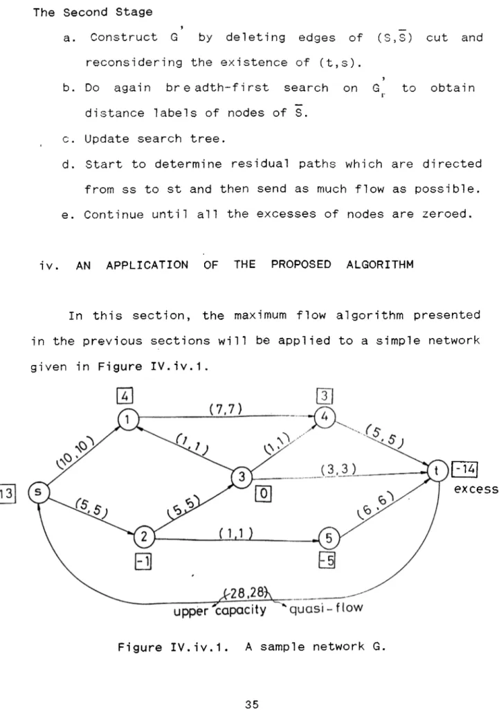
In this section, the maximum flow algor ithm presented in the previous sections will be applied to a simple network given in Figure IV.iv.1.

A ( S , S ) c u t a p p e a r s .

excess

Figure IV.iv.1. A sample network G.

and g steps of the first stage which are given in the previous section are carried out. According to the initial distance labels of nodes, initial search tree shown in Figure IV.iv.3 is constructed. Then whenever a ss-to-st

residual path is found, as much flow as possible is sent

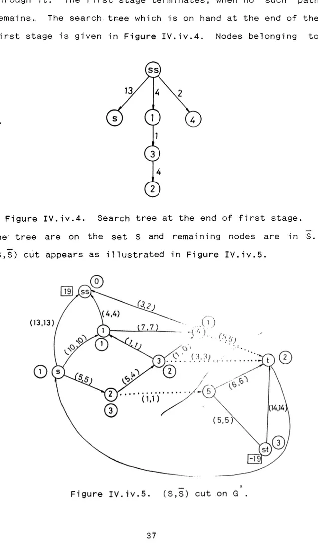
through it. The first stage terminates, when no such path remains. The search, tnee which is on hand at the end of the first stage is given in Figure IV.iv.4. Nodes belonging to

Figure IV.iv.4. Search tree at the end of first stage, the tree are on the set S and remaining nodes are in S, (S,S) cut appears as illustrated in Figure IV.iv.5.

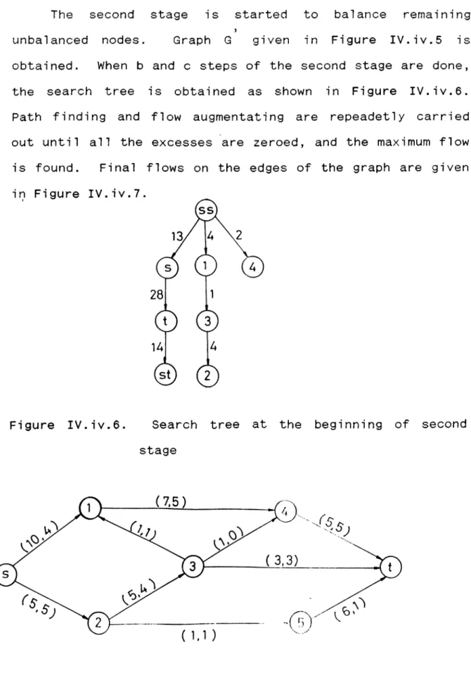
The second stage is started to balance remaining u n b alanced nodes. Graph G given in Figure IV.iv.5 is obtained. When b and c steps of the second stage are done, the search tree is obtained as shown in Figure IV.iv.6. Path finding and flow augmen t atin g are repeadetly carried out until all the exces s e s are zeroed, and the maximum flow is found. Final flows on the edges of the graph are given in Figure IV.iv.7.

Figure IV.iv.6. Search tree at the beginning of second stage

Figure IV.iv.7. Final flows on the edges of G,

V. AN A L T E R N A T I V E PROCEDURE FOR THE SECOND STAGE

The second stage of the a l gor ith m can be carried out by an extended version of Reduce/Relabel step of Goldberg and T a r j a n ’s a l g o ri t h m [13]. In their case, given positive excess nodes and Pr eflow on edges, along shortest paths of positive flow which go from source to unbalanced nodes, flow is reduced to make the positive exces ses zero. In our case, there e xist both positive and negative excess nodes and by means of paths of positive flow source is connected to positive nodes and sink can be reached from negative excess nodes. As m entioned before. Preflow is defined in the subgraph which contains positive excess nodes, source and some of the balanced nodes. Reduce/Relabel step is directly a p p licable to that subgraph. Excess flow is returned to source along short e s t paths. In order to apply Reduce/Relabel step to send flow excess es of negative nodes to sink, a few m o d i f i c a t i o ns have to be made. Subgraph which will be worked on has to be redefined so that for a given Postflow p, E^ = { (i,j) I p(i,j) > 0 } and G^= ( N, E ). By b r e ad t h - fi r st search, starting from sink, initial

p

distance labels of nodes are d e termined s.t. d(t)=0 and 0 < d(i) < n, V i ^ t. Then Reduce/Relabel step becomes:

Reduce: Select any node j s with 0 < d(i) < n and e(j)<0. Select any edge (j,i) e Ep with d(i) = d(j) - 1. Send

S = min { le(j)l , p(j,i) } units of flow from j to i. If

5 is equal to le(j)!, step is excess zeroing otherwise

excess non-zeroing.

Relabel: Select any node j with 0 < d(i) < n . Replace d(j) = min { d(i) + 1 , 1 (j,i) e }.

They have shown that time requirement of that step is 2

always smaller than o( n m) which dominates the time com p l e x i ty of their algorithm. When they have used the Dynamic Trees , they have reduced the time complexity to o( nmlog(n^/m) ). Even in that case, time requirement of that step is smaller than above bound. Hence it is sure that running time of our Reduce/Relabel stage will be smaller than o( nmlogn ) which is the smallest bound we obtained in this study. T herefore this does not improve the overall running time of our algorithm.

C H A P T E R V

DYNAMIC TREE VERSION OF THE ALGORITHM

The running time of the proposed m axi mum flow al gorithm 2

is o(n m). A c t i v it i e s of distance label updating require o(nm) time. Time spent in excess zeroing and non-zeroing

2

pushes is o(n m) and it dominates overall time complexity of our algorithm. If time required to push flow along residual paths from su p e r so u r c e to supersink is reduced from o(n m) to o(nmlogn), overall com plexity of the algo rithm will be reduced. Therefore, our further effort will be concen t r a te d on that. We adopt and apply S l e a t o r - T a r j a n ’s dynamic tree data s tructure to handle pushing steps more e f f i c i e n t l y and obtain a bound of o(nmlogn).

In dynamic tree structure, tree ope ratio ns are defined and used either to get information from the tree or struct u r a ll y update the tree. Tree oper ati ons that will be used in this version are listed below.

p a r e n t ( i ) r o o t ( i ) c a p ( i ) m i n c a p C i ) u p d a t e ( i , x ) l i n k ( i , j , x ) cu t ( i ) capac i ty of the j whose edge m i n i m u m residual of path which returns the p a rent node of i . If i is the root, null is returned,

return root of the tree c o n t a i n i n g node i .

return the residual edge (parent(i),i). return the node (p a r e n t (j ) , j ) has c a p a c i t y a mong edges goes from root to node i.

update residual c a p a c i t i e s of edges on the tree path from root to node i by addi n g x amount to each of them .

co m b i n e trees c o n t a i n i n g node i and j by a d d i n g new edge (i>j) with residual c a p a c i t y x, m a k i n g i be the parent of j .

div i d e the tree c o n t a i n i n g node i

into two trees by d e l e t i n g the edge (p a r e n t (i ) , i ), return residual capac i tу of it.

Among them, root(i), mineap(i), cap(i) are used to get information from tree, others change the tree structure. Cut(i), link(i,j,x), cap(i) o p e rations are carried out at o(1) time per operation. Update(i,x), mincap(i), root(i) require o(n) time per o peration in the worst case. Dynamic thee s t ructure handles each o peration in o(log n) time, if tree contains at most n nodes at any time.

The algo r it h m main t a i n s a collection of disjoint trees. Each node has a single parent node and several children nodes. We assign a pointer variable point(i) to each node i. If point(i) is 1, node is a candidate node to enlarge tree, othe r w i se it is not. Initially supersource is the only cand i da t e node and cap(i) of each node is equal to

infinity indicating that each node is a tree of single node. The dynamic tree version of the algori thm is as

f o i l o w s .

Step 1. If there is a cand i date node go to Step 2, othe r w is e compute residual capacity of each edge and STOP.

Step 2. Take a candidate node i , s. t. poi nt(i) = 1 . If there is an edge (i , j ) in edge list of i s. t . d(j)=d(i)+1 and r (i , j ) > 0, go to Step 3.

Step 3,

O t h e rw i se point(i)=0 and go to Step 1.

If j = S t , go to Step 4, otherwi se go to Step 5.

step 4. Enlarge tree from node i, by making i the parent of j and performing 1 i n k ( i ,j ,r (i ,j )). Node j becomes an other c andidate node, point(j)=1. If parent(j) still is a c andidate node, go to Step 2. Step 5. A path f rom su p e r s o u r ce to supersink is found,

then a flow is sent thru. Let k = m i n c a p ( s t ), then A =cap(k) and p e rform update(st, - A ). Go to Step 6.

Step 6. Delete edges with zero residual capacities. Repeat following step until cap(k) > 0 where k = m i n c a p ( s t ) .

Let k = m i n c a p ( s t ) , p e rform cut(k) and update distance label of node k. If node k has to be relabeled, then apply cut(i) and update(i, ■» ) operation to each node of sub-tree that is d i s c o n n e c t e d from the search tree. After relabeling of node k, update their distance labels.

Then, go to Step 1.

Lemma V.1: Time com pl e x i t y of the dynamic tree version of the a l go r i t h m is o(n°m°logn°) where n*^=(n+2) and m°=(m+n+1).

Proof: Since each push is a s aturating type and reduces residual capacity of at least one edge to zero, number of pushing steps is equal to number of cut operations. Time required by cut o p e rations is o(n°m°).

Total number of link operations is (n°+n°m°). Each node

initially can be linked to the tree once. In addition to that, every node which was disconne cted from the tree can later be linked again. This reasoning gives the above bound. Total number of link op e rations gives an upper bound to the number of times nodes become candidate. It is o(n°+n°m°).

Total relabeling time is o(n°m°) and total time spent in replacement steps is again o(n°m°).

The number of excess zeroing and non-zeroing pushes gives number of paths from ss to st. To assign a bound to o perations of Step 5, we use that result. Hence update operations require o(n m logn ) time.

Total c o m plexity of the a lgorithm is o ( n ° m ° l o g n ° ) . ■

We obtained the order of Sleator and T a r j a n ’s algorithm [21]. Modified Dynamic Tree version of the al gorithm is applied twice on the residual graph. The overall running time of the proposed m a x i m u m flow a lgo rithm is o(nmlogn).

C H A P T E R VI

CONCLUSIONS AND FUTURE RESEARCH

In this study, we tried to approach the classical m aximum flow pr oblem from a different point. The idea behind the a l go r it h m was originated from the following intuitive fact. If the flow on each edge of the graph is equated to upper capacity on that edge , in order to obtain a feasible and optimal flow, flows on some of the edges have to be reduced. Our algo r i t h m answers the question by how much flows on the edges have to be reduced.

A l g o r i t h m defines m i n-cut first, then finds max-flow. When the first stage terminates, dual opti mum solution will be on hand, but, primal o p t i m u m solution will not. The task of the second stage is to find primal op timum solution of a given dual optimum. It is a general question, whether there is a relation between the procedure of the second stage and Dual Simplex method.

We wonder w hether two stages of the a lgorithm can be combined and handled together. In that case, it will be di fficult to define min-cut before obtaining max-flow.

2 The running time of the proposed a l gor ith m is o( n m ). We have used a modified version of. Dynamic Tree data structure of Sleator and Tarjan, and time complexity of the a lg o r i t h m is reduced to o( nmlogn ). It is applied two times on two graphs which have equal size in terms of n and m. Ther ef o r e overall complexity of maxi mum flow a lgorithm is o( nmlogn ).