Rate-Distortion Efficient Piecewise Planar 3-D Scene
Representation From 2-D Images
Evren ˙Imre, A. Aydın Alatan, Member, IEEE, and U˘gur Güdükbay, Senior Member, IEEE
Abstract—In any practical application of the 2-D-to-3-D con-version that involves storage and transmission, representation effi-ciency has an undisputable importance that is not reflected in the attention the topic received. In order to address this problem, a novel algorithm, which yields efficient 3-D representations in the rate distortion sense, is proposed. The algorithm utilizes two views of a scene to build a mesh-based representation incrementally, via adding new vertices, while minimizing a distortion measure. The experimental results indicate that, in scenes that can be approxi-mated by planes, the proposed algorithm is superior to the dense depth map and, in some practical situations, to the block motion vector-based representations in the rate-distortion sense.
Index Terms—Mesh generation, 3-D scene reconstruction, 3-D scene representation.
I. INTRODUCTION
B
UILDING 3-D scene representations from 2-D images is an active topic due to the prospect of high-profile ap-plications, such as automatic model building, multiview video compression, and 3-D TV. There are already several end-to-end systems that obtain a 3-D model of the imaged scene from a 2-D image sequence through structure-from-motion (SfM) tech-niques [1]–[4]. Typically, an SfM algorithm recovers the 3-D lo-cations of the salient point features in a scene, i.e., a sparse pointcloud. This point cloud can be considered as samples from the
surface of the scene [5]. These samples may also contain infor-mation about the scene texture.
The sampling interpretation raises two important issues: • Sampling density: The sampling density should adapt to
the surface complexity, as undersampling leads to distor-tion, and oversampling is a hazard to efficiency. The latter is important for the storage and the transmission of the 3-D scene model.
Manuscript received April 02, 2008; revised October 15, 2008. First pub-lished January 20, 2009; current version pubpub-lished February 11, 2009. This work was supported in part by the European Commission 3DTV Network of Excel-lence Project (FP6-511568) and in part by TÜB˙ITAK under Career Projects 104E022 and 104E029. The associate editor coordinating the review of this manuscript and approving it for publication was Dr. Pier Luigi Dragotti.
E. ˙Imre is with the Centre de Recherche INRIA Nancy Grand Est, Villers-lès-Nancy, France (e-mail: [email protected]).
A. A. Alatan is with the Department of Electrical and Electronics En-gineering, Middle East Technical University, Ankara, Turkey (e-mail: [email protected]).
U. Güdükbay is with the Department of Computer Engineering, Bilkent Uni-versity, Ankara, Turkey (e-mail: [email protected]).
Color versions of one or more of the figures in this paper are available online at http://ieeexplore.ieee.org.
Digital Object Identifier 10.1109/TIP.2008.2010071
• Interpolation function: The interpolant should approxi-mate the dominant structural features on the scene surface adequately. Since a single continuous function can repre-sent only the simplest scenes, the interpolation should be performed with a piecewise function, i.e., patches (usually, a triangular mesh). However, a patch-based parameteriza-tion requires the assignment of each sample to a patch, which is a problem complicated by the absence of a unique neighborhood relation for 3-D points.
In the literature, the first issue is addressed usually by oper-ating in a fine-to-coarse fashion, i.e., by removing vertices as long as the distortion between the original and simplified mesh remains below a certain threshold [5]. However, the mesh dis-tortion, alone, is an inadequate error metric when building a 3-D scene model from 2-D images, as it ignores another im-portant measure of error: the corresponding visual distortion on the available images of the scene.
As for interpolant, there exists a wide range of alternatives from nonuniform rational B-splines (NURBS) to radial basis functions [6]. However, for many real world scenes, planes pro-vide a sufficiently accurate approximation with the additional benefit of compact parameterization. A noteworthy example for piecewise planar scene reconstruction from a point cloud is [7], in which a point cloud is divided into cells, and a plane is fit to the points in each cell. In [8], a similar approach is employed to recover the collection of homographies, or equivalently, the scene planes, describing the feature correspondences in two im-ages.
Modern graphics hardware can render triangular patches; therefore, it is a good choice as interpolant. Moreover, when
Delaunay triangulation [9] is employed, the vertices alone are
sufficient to represent a mesh; thus, no additional resources for representing the plane boundaries is needed, unlike the image [8], [10] or space segmentation [7] based methods.
The sampling interpretation of the problem highlights the conflicting requirements on the size and the quality of a scene representation, hence, implies that the problem should be studied in a rate-distortion framework. Reference [11] is among the first attempts to achieve a rate-distortion efficient solution, by using a Markov random field formulation to minimize an objective function, which consists of terms corresponding to the image distortion, and the rate of a dense depth map representing the scene. On the other hand, image-based triangulation (IBT) is another powerful technique to achieve the same goal with triangular meshes [12].
The basic IBT algorithm [12] refines an initial mesh via edge swaps to minimize the error between an image and its prediction from a reference image. In [13], the method is robustified against
local minima through a simulated annealing procedure that is re-inforced with a rich arsenal of tools involving adding, removing and perturbing vertices, and modifying the mesh edges. Finally, in [14], IBT is applied to stereo image coding, to represent a disparity map, by adding new vertices to the places where the distortion is largest.
The work presented in this paper employs an IBT approach, enhanced with the features presented in Section II. It has two main contributions: a rate-distortion efficient algorithm that builds a mesh-based representation from two images of a scene, and an experimental comparison of various dominant scene representation techniques within the context of 3-D scene mod-eling from 2-D images. To the best of the authors’ knowledge, there is no prior work addressing any of these issues in the literature.
The organization of the paper is as follows: In the next sec-tion, some design considerations for a generic rate-distortion ef-ficient scene reconstruction algorithm, and the extent to which the existing IBT algorithms fulfill them are discussed. The gen-eration of the mesh and its refinement through nonlinear min-imization are explained in Sections III and IV, respectively. In Section V, various aspects of the algorithm are studied via ex-periments, and a comparison of the rate-distortion performance with dense depth map and block motion vector representations is presented. Section VI concludes the paper.
II. DESIGNCONSIDERATIONS
In order to design an algorithm that yields both accurate and rate-distortion efficient representations, the following features are identified as desirable.
• Piecewise planar reconstruction with triangular patches: Triangular patches provide an efficient and
sufficiently accurate approximation for most real-world scenes [17] and offer computational advantages [15]. • Coarse-to-fine operation: The best-known algorithms
in the literature, such as [5], [12], and [13], operate in a fine-to-coarse fashion. The disadvantages of this approach are twofold. First, for the equivalent problem of finding a minimal set of vertices that describes a scene at a given distortion level, more vertices imply a more complex error surface. Second, it is computationally inefficient to estimate some entities to be discarded later. Operating in a coarse-to-fine fashion avoids both of these problems. • Feedback from representation to feature extraction:
Coarse-to-fine operation requires a feedback path from representation back to feature extraction, to convey the directives of the representation block regarding to which parts of the structure require refinement. This mechanism adapts the sampling density to the surface complexity. Only in [14] is such a mechanism considered.
• Capability to update both structure and camera: The methods in the literature assume that the true values of the internal and external calibration parameters for the cameras are available and attribute any error to insufficient number of vertices [14], incorrect connections in the mesh [12],
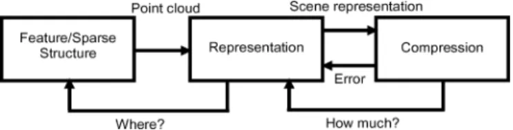
Fig. 1. Framework for rate-distortion efficient piecewise planar 3-D recon-struction.
and sometimes to errors in the vertex positions [13]. How-ever, when building a 3-D scene model from 2-D images, both the cameras and the point cloud are estimated from the input data. It is possible to eliminate any sensitivity to in-ternal calibration errors by operating in a projective frame. However, the algorithm should be able to cope with the er-rors in the camera matrix estimates, as well.
The operation of a rate-distortion efficient algorithm that ad-heres to the above specifications is illustrated in Fig. 1 for a coding application. The feature extraction and sparse structure estimation block computes a point cloud as a sparse representa-tion of the scene, which is upgraded to a piecewise planar recon-struction in the representation module. Then, the compression block encodes the representation, and returns the coding error and the remaining bit budget. The representation block deter-mines the patches that require further refinement and sends a request to the feature extraction block for new scene features in these regions. Among these new features, the one that is in least agreement with the current scene representation is added to the point cloud, which is, in turn, used to update and refine the rep-resentation. The feedback path ensures that an increase in the rate is accompanied by an increase in the representation quality, i.e., the algorithm operates in a rate-distortion efficient fashion.
III. PIECEWISEPLANARRATE-DISTORTIONEFFICIENT3-D SCENERECONSTRUCTION
A. Scene and Image Model
The 3-D scene is modeled as a connected surface, , which is composed of a union of disjoint triangular patches , i.e.,
(1)
The projection of from to via the projection op-erator is defined as
(2) where denotes the projection, represents a 3-D scene point and is its projection to 2-D by . Both and are repre-sented by homogeneous coordinates, and the symbol denotes homogeneous equivalence. is defined as
otherwise
(3)
for an ordering function , a point on and its projection . When rendering a view of a scene, the projection operator
is defined by the camera acquiring the view, and is known as the camera matrix. In this case, is specified as the distance of a point in to the image plane of the camera, which is also defined by . Equation (3) states that among all points which are on and projected to , only the one closest to the image plane is an element of . In other words, is 1 when is visible to the camera.
A discrete image can be expressed as a sampling of the projection of by a regular integer grid, i.e.,
(4) (5)
where denotes the Dirac delta function.
Finally, the points in any two projections of , , and are related by [15]
(6) where is an element of and is its correspondence in .
is defined as [15]
(7) where and are the camera matrices of the cameras imaging and , respectively. is the null vector of , and is the vector denoting the plane equation of . The symbol “ ” stands for the pseudo-inverse operation.
B. Rate and Distortion
In this work, rate is defined as the number of vertices. Al-though this quantity and the size of the compressed mesh are not exactly equivalent, for the meshes produced by the proposed system, there exists an almost linear relation, as observed in Fig. 9.
The distortion is measured by the sum of squared intensity
differences (SSD) between a target image, , and its predic-tion, . This can be expressed as the sum of distortions of the projections of the individual scene planes, i.e.,
(8)
where
(9) Assuming an independent zero mean Gaussian noise process affecting the intensity values of each pixel, a Lambertian re-flectance model, constant lighting, and given the true 3-D point coordinates and the camera matrices, the triangulation with the minimum SSD is the maximum-likelihood solution for the IBT problem [12], [13]. However, SSD is disproportionately sensi-tive to geometric errors [26], i.e., a small error in the 3-D co-ordinates of a point, or in the camera matrix may cause a large
increase in SSD, and in certain situations, it is poorly related to the perceived distortion (e.g., a 1-pixel shift). Despite these drawbacks, due to the lack of a better and equally widely ac-cepted alternative [27], SSD is adopted as the distortion metric. The effects of this choice on the 3-D model estimation are fur-ther discussed in Section V. However, the algorithm itself is in-dependent of the choice of distortion metric, therefore, different image distortion metrics can be employed depending on the ap-plication.
C. Proposed Method
The algorithm requires two images as input: a target and a
reference image. The reference image and the current scene
rep-resentation are used to compute a prediction of the target image. The scene representation is built incrementally through the ad-dition of new vertices in a way to reduce the distortion defined in the previous section. Given the assumptions in Section III-B and the further assumption that (6) is sufficient to construct the target image from the reference image and the true scene model, the procedure should terminate when the distortion reaches to zero. However, in practice, the assumptions about lighting and illumi-nation are commonly violated and the true values of the struc-ture and the camera parameters are not available. Moreover, the reflections, occlusions, disocclusions [12], and the performance of the intensity interpolation algorithm (in this work, bilinear interpolation [30]) limit the usefulness of (6). All these factors give rise to an irreducible error.
The initial scene representation and the camera matrices can be computed from the reference and the target images via conventional structure-from-motion (SfM) techniques [4], [15]. However, it is also possible to use any initial structure and camera estimates from other sources.
The 2-D triangular mesh representing the scene is constructed by performing a Delaunay triangulation on the projection of the point cloud to the image plane of the target image. This mesh is then lifted to 3-D [17]. This operation may compromise cer-tain optimality properties of Delaunay triangulation [18], specif-ically, those that guarantee the maximization of the minimum angle of the mesh. Delaunay triangulation owes its popularity to this property, as in practice, the closer the members of a triangu-lation to equilateral triangles are, the more accurate the surface models tend to be [17]. However, lifting may transform a 2-D equilateral triangle to a 3-D “sliver,” a structure that is seldom encountered in real world scenes and, thus, is unlikely to model the corresponding portion of the surface correctly. On the other hand, the scene representation obtained in this fashion is pro-jective invariant; hence, invulnerable to the errors in the internal camera parameters.
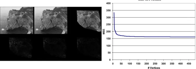
The proposed representation seemingly has an important lim-itation: if a low-texture portion of the scene is not surrounded by a set of salient features (e.g., the sea in Fig. 6), it is not fully contained within the projection of the point cloud, and the cor-responding triangulation. However, regardless of the represen-tation, the only clue to the 3-D position of such a region is the smoothness of the depth field. Therefore, this problem can be solved by propagating the depth values obtained from the mesh
representation into these regions via an iterative-diffusion type dense depth estimation algorithm [29].
The most important stage of the proposed algorithm is vertex selection. Ideally, the chosen vertex should be the one, whose addition to the existing representation minimizes the distortion (which is measured by SSD), i.e., the solution of the following minimization
(10) where denotes the distortion for the surface formed by the addition of to the surface formed by all of the vertices currently in the representation, .
An optimal solution to (10) is often computationally unfea-sible. The proposed method employs a suboptimal solution that relies on the following assumptions.
1) The projection of to the target frame lies within the re-gion that satisfies the condition
(11) 2) projects to a discernible feature in both images. 3) that minimizes (10) also minimizes the symmetric
transfer error (STE) defined as [15]
(12) where and correspond to the projections of to the reference and the target images. is the homography for the scene plane which satisfies the first assumption, and is defined in (7), with being the camera matrix of the reference, and being that of the target camera.
The first assumption can be easily justified, as the triangular patch that corresponds to the region with the largest distor-tion, is likely to be the one whose refinement will improve the representation most [14].
The second assumption allows the reduction of the search space for to a finite set of vertices, therefore, provides im-mense computational savings. It is justifiable, as the discernible features on the images often correspond to the scene corners, which may be residing on scene plane boundaries [28], and whose omission in the representation is likely to contribute to the distortion significantly.
The last assumption stems from the fact that, for a correct match, STE in (12) evaluates the conformity of a vertex to the local planar model, . The implication is that the vertex that is in least agreement with the local planar model causes the most distortion. It is possible to achieve a reduction in the compu-tational cost by several orders of magnitude, by choosing this vertex, instead of the one whose inclusion minimizes (8). A sim-ilar assumption is employed in [14], with regard to maximum disparity error.
The vertex selection procedure is as follows. First, the re-gion with the largest distortion in the target frame is determined. This region and the corresponding region in the reference frame are declared as the search regions. Within these regions, the salient features are extracted by a corner detection algorithm, and matched by guided matching [15]. If no reliable matches are available, the feature extraction step is reattempted with
progressively lower thresholds. If the threshold drops below a minimum beyond which corner detection becomes unreliable, the patch is skipped and the algorithm continues with the patch which has the second largest distortion. Finally, these matches are evaluated by (12), and the pair with the largest STE is used to instantiate the new vertex. Since a false match can also yield a high STE, only the reliable matches should be used in the pro-cedure.
The scene representation, i.e. the current mesh, is updated with the new vertex by using the dynamic Delaunay triangula-tion technique described in [9]. Then, a predictriangula-tion of the target image is rendered by warping the reference image to the image plane of the camera of the target image, via bilinear interpola-tion. If the addition of the vertex indeed improves the represen-tation quality, it is accepted; otherwise, it is rejected.
The algorithm is summarized as follows.
Algorithm: Rate-Distortion Efficient Piecewise Planar Scene Reconstruction
Input: A reference image, a target image, optionally, the initial
structure and camera matrix estimates
Output: A piecewise planar representation of the scene
Until the distortion converges or the bit budget is depleted 1. Determine the patch with the largest distortion via (9). 2. Establish correspondences in the search regions associated
with the patch.
3. Find the feature pair with the least conformance to the patch via (12).
4. Add the corresponding vertex to the representation. 5. If the representation error is reduced, update the mapping,
the collection of homographies, between the target and the reference frame, by (7). Use this mapping to compute a prediction of the target frame via (6), with being a point in the target image, and its correspondence in the reference image. Return to step 1.
6. If the representation error is not reduced, find the feature pair with the next least conformance to the patch via (12). Return to step 4.
IV. MESHREFINEMENT VIANONLINEARMINIMIZATION
The scene representation of the previous section can be im-proved by minimizing (8) with respect to the vertices and the camera parameters. The inclusion of the camera parameters pre-vents the minimization procedure from introducing errors to the structure, to compensate for any inaccuracies in the camera ma-trices.
The minimization problem is formally defined as
(13)
where and denote the target image, and its computed via (6) and (7), respectively. represents the vertices of the mesh and, denotes the camera parameters. is the projec-tion of the scene surface to the image plane of the target camera,
TABLE I
DISTORTIONWITHOUTNONLINEARMINIMIZATION, WITHSTEEPESTDESCENT(SD)ANDWITHSIMULATEDANNEALING(SA)
and is dependent on and . The minimization is subject to the constraint that the area of cannot be decreased.
In order to avoid local minima, (13) is minimized via
sim-ulated annealing [19]. Simsim-ulated annealing tries to improve a
solution through random perturbations. In the proposed algo-rithm, the following perturbation mechanisms are employed.
• Move vertex: All vertex locations are perturbed randomly. • Move camera: Camera parameters are perturbed
ran-domly.
• Add vertex: A new vertex is randomly added to the recon-struction.
• Remove vertex: A vertex is randomly removed from the reconstruction.
The probability of accepting a solution is given as else
(14) where is the cost function, which is defined as the operand of the minimization in (13). In (14), denotes the current so-lution, i.e., the current vertex and the camera parameters, and , the tested solution, which is a perturbation of . If is ac-cepted, and , the temperature parameter, are updated. The update rule for is [19]
(15) where is the update counter, and is the initial value of . Equation (14) implies that a solution with a higher cost still has a certain chance of being accepted; hence, the algorithm can move out of a local minimum.
An accepted solution is further refined via steepest descent [25] with respect to the camera parameters and the vertices. The steepest descent algorithm moves towards the local minimum of the basin in which resides, i.e., in the opposite direction of the gradient of the error surface with respect to . The gradient is approximated by forward differencing. The step size adapts to the local characteristics of the error surface: An improvement in the cost encourages the algorithm to take larger steps. Other-wise, the algorithm reattempts to move from the current solution with a smaller step. Each iteration is composed of two phases: one for optimization with respect to , and the other with re-spect to .
Simulated annealing is a capable, yet computationally in-tensive, procedure. In case of limited computational resources,
steepest descent can be applied directly to the output of the al-gorithm in Section III, without any prior or posterior simulated annealing stage. The extent to which the final representation quality is affected depends on the characteristics of the error surface around the solution. The results in Table I do not identify any of the methods as entirely redundant, therefore, suggest that it is advisable to apply simulated annealing, when it is computationally feasible.
V. EXPERIMENTALRESULTS
The performance and the properties of the proposed algo-rithm are studied by two sets of experiments. In the first set, the algorithm is run on synthetic and real data, in order to study the convergence behavior, and the effects of incorrect vertex and camera parameter estimates. The second set aims to compare the rate-distortion efficiency of the representation produced by the proposed algorithm with that of the dense depth map, and block motion vector-based representations. The section is concluded by an empirical justification of the use of number of vertices as a measure of rate.
A. Piecewise Planar Scene Reconstruction
The piecewise planar reconstruction experiments are per-formed on the following data sets: Peter is a synthetic data with ground-truth camera and structure available. The imaged scene has nine surfaces and 12 vertices. For Venus [20] and
Breakdancers [21], only the camera parameters are known. Palace and Cliff are acquired from TV broadcast; hence, neither
the camera nor the structure is known. Finally, Castle belongs to a collection of photographs of a mostly planar scene taken from various poses.
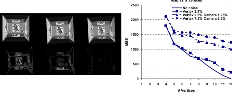
The first experiment aims to explore the effect of noisy ver-tices and camera parameters. The results, presented in Fig. 2, indicate a serious degradation for Peter in the presence of noise, especially when the noise affects the camera parameters. How-ever, as observed in Table I, the nonlinear minimization stage significantly improves the results.
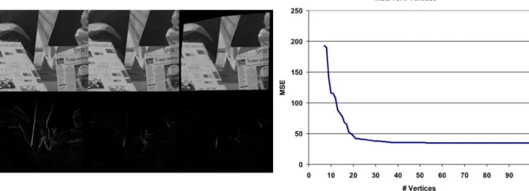
The second experiment seeks to assess the performance of the proposed method when only the camera parameters are known. For Breakdancers, the ground truth camera matrices are avail-able, and for Venus, the optical axes of the cameras are parallel, and the motion is a horizontal translation, therefore, it is pos-sible to compute the exact projective camera pair. The results are presented in Figs. 3 and 4. The black regions correspond to the
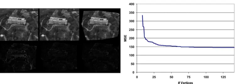
Fig. 2. Experimental results for Peter. Left, top row (left to right): reference, target, and predicted images for 7.5% vertex and 2.5% camera noise case. Left, bottom row (left to right): prediction error at the beginning, before nonlinear optimization, and after nonlinear optimization. Right: representation quality versus # vertices for various noise levels on the vertices and the camera parameters.
Fig. 3. Experimental results for Breakdancers. Left, top row (left to right): reference, target, and predicted images. Left, bottom row (left to right): prediction error at the beginning, before nonlinear optimization, and after nonlinear optimization. Right: representation quality versus # vertices.
parts of the scene that cannot be represented due to lack of fea-tures. The results indicate that Breakdancers and Venus scenes can be represented with approximately 30 vertices at qualities exceeding 30 and 32 dB, respectively. Considering the discus-sion in Sections III-B and III-C, the residual error observed in Table I and Figs. 3 and 4 is expected: The practical limitations of the feature localization, in turn, limit the accuracy of the 3-D points in the point cloud; hence, introduce a base error level that cannot be reduced. The estimates are further degraded by the relatively poor performance of the image rendering procedure at the edges. And finally, the violation of the connected surface assumption has an impact on the performance, as observed at the plane borders in Venus.
The final experiment of the set evaluates the algorithm in the case when both the vertices, and the camera matrices are esti-mated from the data. In MSE calculations, in Palace and Cliff, the parts of the scenes corresponding to TV station logos are not taken into account. Besides, since the inclusion of Castle into
the data set serves to study the performance of the algorithm in mostly planar scenes, the contribution of the trees, a region that cannot be reliably approximated by planes, and the sky to the distortion are also discarded. The experimental results are pre-sented in Figs. 5–7 and Table I.
In case of unknown camera and structure, the algorithm still converges, albeit at a slower rate and to a higher residual error. These observations can be attributed primarily to the inaccura-cies in the estimation of the camera and vertex positions. The upwards trend in the residual errors from the “known camera and vertices” to the “unknown camera and vertices” case lends support to this interpretation. It is also the best addressed one, as unreliable vertices are eliminated during the construction of the representation, and the nonlinear minimization stage attempts to improve the vertex positions and cameras by random displace-ments.
Another source of error stems from the violation of one of the fundamental assumptions in this study: the intensity values
Fig. 4. Experimental results for Venus. Left, top row (left to right): reference, target, and predicted images. Left, bottom row (left to right): prediction error at the beginning, before nonlinear optimization, and after nonlinear optimization. Right: representation quality versus # vertices.
Fig. 5. Experimental results for Castle. Left, top row (left to right): reference, target, and predicted images. Left, bottom row (left to right): prediction error at the beginning, before nonlinear optimization, and after nonlinear optimization. Right: representation quality versus # vertices.
of the target image can be computed from those of the refer-ence image perfectly, given the correct geometry and camera positions; thus, the minimization of (8) leads to better estimates of these parameters. The assumption generally holds for the parts of the scene with low intensity variation, or that are dis-tant from the camera. However, when the images are taken from considerably different positions, as discussed in Section III-C, occlusions, disocclusions and reflections on the reflective sur-faces, such as windows, weaken this assumption, cause a larger residual error (but, not necessarily a worse result, if SSD is ill-suited as a distortion metric for the target application) and give rise to local minima, in which the optimization process may be trapped, despite the use of simulated annealing. The proposed algorithm cannot avoid this problem: it is not equipped with any tools to deal with the errors not caused by the camera and the vertex parameters, except for significant structure deformations, which are likely to degrade the representation. Therefore, the re-sult is one of the plausible, but erroneous, interpretations of the information contained in the 2-D image pair [13].
A simple indicator of the validity the “computability” as-sumption is the difference of the mean intensities of the target and the reference frames, i.e.,
(16)
where and are reference and target images, respectively, and is the number of pixels in an image. In Castle, the reflec-tions on the windows, and the change in illumination cause a of 7, whereas in Cliff and Palace, is below 1, a rather small value. Therefore, the predictability of the intensity values of the target frame from the reference frame in Castle is less than that in Cliff and Palace; hence, the residual error should be higher. The experiments confirm this hypothesis.
A related problem is the limitations of the simple image ren-dering method (i.e., warping and bilinear interpolation) utilized in the experiments. This method has no special provisions for
Fig. 6. Experimental results for Cliff. Left, top row (left to right): reference, target, and predicted images. Left, bottom row (left to right): prediction error at the beginning, before nonlinear optimization, and after nonlinear optimization. Right: representation quality versus # vertices.
the edges, at which the distortion is concentrated due to the over-sensitivity of SSD to minor errors in the vertex coordinates and camera matrix errors. Moreover, it also blurs the highly tex-tured regions. However, if the distortion levels achieved with this basic rendering method are inadequate for the target ap-plications, it is possible to replace it with a more sophisticated method, such as [31].
The final major source of error is the incorrect connections between the vertices, leading to instantiation of planes nonex-istent in the scene. These planes model the local structure erro-neously, and introduce artifacts, such as bending of planar sur-faces, an effect that can be detected by its action on straight lines. Two causes for such erroneous models are identified as mesh construction in 2-D, and missing vertices. The former is the price paid for projective invariance: since the mesh is con-structed in 2-D, it is possible that two far-away and unrelated vertices in 3-D might be projected to nearby locations. In that case, these points are connected, forming one edge of a plane nonexistent in the scene. The latter is caused by the limita-tions of the feature extraction and matching procedures, as it is not always possible to recover a corresponding feature pair set both sufficiently dense enough to describe the boundary of the scene planes correctly, and accurate enough for reliable 3-D po-sition estimation. The lack of features degrades the results in two ways: the estimated plane boundaries might not coincide with the actual boundaries, and the vertices belonging to the interior of a plane might be connected to the vertices of other planes, and give rise to planes nonexistent in the scene.
The influence of these artifacts on the distortion depends on the size of the afflicted patches and the texture they contain. As long as there is a strong intensity variation, such a group of patches causes a high SSD, therefore, is selected for refinement and broken down into smaller patches through the addition of new vertices. The increased level of detail reduces the size of the region affected by the artifact, or removes the artifact com-pletely. However, in case of flat patches, despite the high error at the boundaries, the total distortion of the patch may be rel-atively low. In this case, the nonlinear minimization stage may be able to reduce the distortion more, by moving a vertex of a
smaller, yet highly textured region, at the expense of a large but flat patch. Although this behavior reduces the overall distortion, it does not necessarily yield a more accurate scene representa-tion.
B. Rate-Distortion Performance
In the second experiment set, the rate-distortion performance of the proposed algorithm is compared with that of the block motion vector (BMV) and dense depth map (DDM) representa-tions. A DDM representation describes a scene by the distance of each scene point corresponding to a pixel in the reference image, from the image plane of the reference camera. A BMV representation tiles the reference frame into blocks, and assigns a 2-D motion vector to each block. Since each 2-D motion vector defines a mapping between a block in the reference frame and its correspondence in the target frame, the BMV representation can be considered as a kind of 3-D scene representation. This mapping can be expressed as
(17)
where is a pixel in the target block and is a pixel in the refer-ence block. and stand for the block motion vector. Equation (17) is a special case of (6), i.e., the mapping relating the blocks in both images is a homography, hence, the part of the 3-D scene projecting to the block is approximated as a plane. Therefore, the BMV representation models the 3-D scene as a collection of planes. Besides, BMV-based prediction plays an important role in state-of-the-art stereo and multiview image and video com-pression algorithms; thus, comparing its performance to that of the proposed algorithm serves to assess the suitability of piece-wise planar scene models for such applications.
The rate of the proposed algorithm is obtained by com-pressing the resulting mesh with topological surgery [16], a mesh encoder which is a part of the ISO MPEG-4 standard. The vertices are compressed with 20 bits. The distortion is measured by MSE. For a fair distortion comparison, only the regions that could be represented by all three methods are
Fig. 7. Experimental results for Palace. Left, top row (left to right): reference, target, and predicted images. Left, bottom row (left to right): prediction error at the beginning, before nonlinear optimization, and after nonlinear optimization. Right: representation quality versus # vertices.
TABLE II
COMPARISON OFCOVERAGE ANDRATE-DISTORTIONPERFORMANCES INMUTUALLYCOVEREDREGIONS. ABOLDVALUEINDICATES ASUPERIOR
RATE-DISTORTIONPERFORMANCE. CoverageIS THERATIO OF THEIMAGETHAT ISREPRESENTED BY THEBMVAND THEPROPOSEDMETHOD,
TO THEENTIREIMAGE, RESPECTIVELY
included in the error calculations. Table II lists the coverage ratio attained by the proposed and the BMV-based approaches. The DDM representation can cover the entire image.
In order to generate a DDM, the algorithm described in [10] is employed. This algorithm is a region-based global method, that models a scene as a collection of planes. Being a global method, the algorithm is superior to local methods [29], and the use of image segmentation allows it to handle plane boundaries and discontinuities more successfully [33], [34] than other al-gorithms in this class. Moreover, the algorithm goes beyond the conventional region-based plane sweeping methods [34]–[36] by employing angle sweeping, a feature which makes it espe-cially suitable for planar scenes. The algorithm is competitive against the best 25 algorithms in the Middlebury benchmarks [33].
The rate-distortion curve for the DDM-based approach is obtained by compressing the DDM, which is stored as a bitmap image, by the ITU-T H.264/ISO-IEC 14496-10 encoder [22], [23], for different compression levels [24], [32]. The decom-pressed depth map is used to construct the target image from the reference image, by warping and bilinear interpolation, as described in Section III-C. The rate-distortion curves of the proposed method and the DDM representation are depicted in Fig. 8. In order to provide an upper bound to the performance,
the distortion values for the lossless-compressed depth maps are also presented in Table III.
For the computation of the rate-distortion performance of the BMV representation, the ITU-T H.264/ISO-IEC 14496-10 encoder is employed, due to its advanced BMV estimation and compression engine. Motion vectors are encoded in a lossless fashion by using content-adaptive binary arithmetic coding (CABAC) [22]. The encoder is configured to predict a target frame from a reference frame, i.e., to encode only two frames. In order to encourage the use of BMV, intraframe mode is suppressed by setting its quantization parameter to 50 (i.e., the intraframe predictions are degraded to increase the likelihood of the selection of the interframe mode, at the inter/intraselection step). For the rate and distortion calculations, only the blocks encoded by the interframe mode, i.e., BMV, are taken into account. These blocks are identified from the trace file. In the experiments, the operational value of the rate is used loosely as the bit budget. The results for 5 different data sets are presented in Table II.
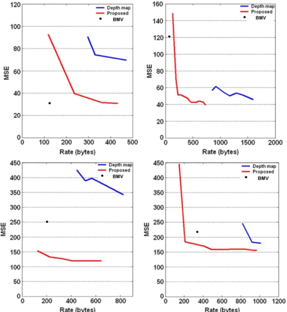
The dense depth map experiments clearly indicate the superi-ority of the proposed mesh-based method: as observed in Fig. 8, in all 4 experiments, the DDM method is outperformed by the proposed method. Moreover, Tables III and IV indicate that, in
Fig. 8. Comparison of rate-distortion performance of the proposed method, depth map and block motion vector representation (H.264). Top left: Venus. Top right: Breakdancers. Bottom left: Cliff. Bottom right: Castle.
TABLE III
DISTORTION FORDENSEDEPTHMAPSAFTERLOSSLESSCOMPRESSION
rate, and in Castle, the dense depth map method can achieve an equivalent distortion only at a much higher rate. Relatively high-bit-rate of the DDM representation might be hinting that it is a favorable trade-off to represent a planar scene with a small number of high precision vertices, instead of a large number of low-precision transform coefficients. As for the distortion, there are two depth map-specific mechanisms in effect: compression artifacts and quantization losses. The former smooths depth dis-continuities, causing distortions that contribute significantly to
the final prediction error. The latter arises from the fact that the value of a pixel comes from a discrete set of intensity levels; thus, continuous depth values must be quantized. The quantiza-tion errors become more dominant as the depth range increases. In the experiments, uniform quantization is employed. These are in addition to the image rendering method-related distortions which are already discussed in Section V-A, and which can be remedied through the use of more sophisticated rendering al-gorithms [31]. However, as long as the same rendering mech-anism is used for both dense-depth and the proposed methods, the above discussion remains valid.
Block motion vector experiments present a more complex picture, which makes sense once the strengths and weaknesses of the BMV representation are considered. BMV provides a 2-D scene representation, as it utilizes 2-D motion vectors to de-scribe the scene. Therefore, the descriptive power of the BMV representation degrades when the effect of depth is non-negli-gible, e.g. in scenes with a large depth range. On the other hand, the piecewise planar mesh representation proposed in this work
TABLE IV
RATE ATWHICH THEPROPOSEDMETHOD AND THEDENSE-DEPTHMAP
METHOD HAS THESAMEDISTORTION
is a 3-D scene representation; thus, it can successfully handle such cases. Another effect of the depth range becomes evident from its interpretation as disparity range. A large depth range suggests a larger variation of the depth; hence, the disparity values within a block, and a stronger violation of the uniform disparity assumption of the BMV. A comparison of the perfor-mance of the BMV and mesh-based representations in the large depth-range data, such as Cliff and Palace, and the small-depth range data, e.g., Venus and Breakdancers supports these conclu-sions: the proposed algorithm outperforms the BMV approach in the former case, and is inferior to it in the latter, especially in
Venus.
Another issue that should be considered is the case of scenes with disconnected planes. The BMV representation successfully handles such scenes, as each block is registered independently from its neighbors; therefore, the scene is modeled as a collec-tion of disjoint planes. On the other hand, the proposed algo-rithm does not accommodate for such cases, which is another factor that contributes to its inferior performance to the BMV representation in Venus, which is a scene composed of disjoint planes.
C. Relation Between the Number of Vertices and Rate
The rate of the representation is determined by the size of the compressed mesh. The topological surgery method encodes the mesh edges very efficiently. Therefore, it can be assumed that only the number and the spatial distribution of the vertices determine the rate. The influence of the latter stems from the predictive coding scheme employed to encode the coordinates of the vertices [16].
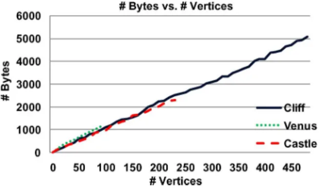
In order to explore the relation between the number of vertices and the size of the compressed mesh, the number-size pairs for each member of the sequence of increasingly complex meshes generated by the algorithm for Cliff, Castle and Venus are plotted in Fig. 9. The observed linear dependency to the number of ver-tices suggests that similar distribution characteristics are pre-served throughout a mesh sequence. Considering that the opti-mization process is driven by SSD, this is expected: at each step, the algorithm picks the vertex to be added from the patch with the highest total image error. Therefore, larger patches are more likely to be selected. Since such patches are generated usually in sparsely populated regions of the mesh, it can be argued that the algorithm tends to maintain a spatially balanced vertex dis-tribution.
Fig. 9. Relation between the number of vertices of a mesh and its size in bytes after compression via topological surgery, for the sequences of meshes in the experiments in Section V-B. Breakdancers is totally obscured by other plots; hence, it is not included.
VI. CONCLUSION
In this paper, an algorithm that builds a piecewise planar scene representation from 2-D images is proposed. The algo-rithm seeks a favorable point on the rate-distortion curve by refining an initial mesh through the addition of new vertices, whose locations are determined by the representation error measured by (8). The representation is further refined by non-linear minimization via simulated annealing. The algorithm itself is independent of the exact choice of distortion metric and the image rendering method, so it can be customized to meet the needs of different target applications. The experimental results indicate that, in scenes that can be modeled by planes, the algorithm is superior to the dense depth map representation in rate-distortion sense. When compared to the BMV represen-tation, the proposed method yields better results under certain conditions, such as connected surfaces and large depth range. Although the algorithm is a significant step towards rate-distor-tion optimal 3-D scene representarate-distor-tion, it suffers from inaccurate vertex and camera estimates, illumination changes, and mesh edges not coinciding with actual scene plane boundaries.
ACKNOWLEDGMENT
The authors would like to thank S. Gedik and C. Çi˘gla for their help with the dense depth map and the BMV experiments.
REFERENCES
[1] D. Nister, “Automatic passive recovery of 3D from images and video,” in Proc. 2nd Int. Symp. 3D Data Processing, Visualisation and Trans-mission, Thessaloniki, Greece, 2004, pp. 438–445.
[2] M. Pollefeys, “Automatic 3D modeling with a hand-held camera im-ages,” presented at the 2nd Int. Symp. 3D Data Processing, Visualisa-tion and Transmission, Tutorial, Thessaloniki, Greece, 2004. [3] T. Rodriguez, P. Sturm, P. Gargallo, N. Guilbert, A. Heyden, F.
Jau-regizar, J. M. Menendez, and J. I. Ronda, “Photorealistic 3D recon-struction from hand-held cameras,” Mach. Vis. Appl., vol. 16, no. 4, pp. 246–257, 2005.
[4] E. ˙Imre, S. Knorr, B. Özkalayci, U. Topay, A. A. Alatan, and T. Sikora, “Towards 3D scene reconstruction from broadcast video,” Signal Process.: Image Commun., vol. 22, no. 2, pp. 108–126, 2007. [5] H. Hoppe, T. DeRose, T. Duchamp, J. McDonald, and W. Stuetzle,
“Surface reconstruction from unorganized points,” in Proc. ACM SIG-GRAPH, 1992, pp. 71–78.
[6] A. A. Alatan, Y. Yemez, U. Güdükbay, X. Zabulis, K. Müller, Ç. E. Erdem, C. Weigel, and A. Smolic, “Scene representation technologies for 3DTV- a survey,” IEEE Trans. Circuits Syst. Video Technol., vol. 17, no. 11, pp. 1587–1605, Nov. 2007.
[7] K. Schindler, “Spatial subdivision for piecewise planar object recon-struction,” in Proc. SPIE and IS&T Electronic Imaging-Videometrics VIII, Santa Clara, CA, 2003, pp. 194–201.
[8] A. Bartoli, P. Sturm, and R. Horaud, A Projective Framework for Struc-ture and Motion Recovery From Two Views of a Piecewise Planar Scene INRIA Rhone-Alpes, Saint Ismier, Tech. Rep. RR-4970, 2000. [9] O. Devillers, S. Meiser, and M. Teillaud, “Fully dynamic Delaunay
tri-angulation in logarithmic expected time per operation,” Comput. Geom. Theory Appl., vol. 2, no. 2, pp. 55–80, 1992.
[10] C. Çi˘gla, X. Zabulis, and A. A. Alatan, “Region-based dense depth extraction from multiview video,” in Proc. 2007 IEEE Int. Conf. Image Processing, San Antonio, TX, vol. 5, pp. 213–216.
[11] A. A. Alatan and L. Onural, “Estimation of depth fields suitable for video compression based on 3-D Structure and motion of objects,” IEEE Trans. Image Process., vol. 6, no. 6, pp. 904–908, Jun. 1998. [12] D. D. Morris and T. Kanade, “Image consistent surface triangulation,”
in Proc. IEEE Conf. Computer Vision and Pattern Recognition, Hilton Head Island, SC, 2000, pp. 332–338.
[13] G. Vogiatzis, P. Torr, and R. Cipolla, “Bayesian stochastic mesh op-timization for 3D reconstruction,” in Proc. 14th Brit. Machine Vision Conf., Norwich, CT, 2003, vol. 2, pp. 711–718.
[14] J. H. Park and H. W. Park, “A mesh based disparity representation method for view interpolation and stereo image compression,” IEEE Trans. Image Process., vol. 15, no. 7, pp. 1751–1762, Jul. 2006. [15] R. Hartley and A. Zisserman, Multiple View Geometry in Computer
Vision. Cambridge, U.K.: Cambridge Univ. Press, 2003.
[16] G. Taubin and J. Rossignac, “Geometric compression through topolog-ical surgery,” ACM Trans. Graphics, vol. 17, no. 2, pp. 84–115, 1998. [17] M. de Berg, M. van Kreveld, M. Overmars, and O. Schwarzkopf,
Com-putational Geometry: Algorithms and Applications, 2nd ed. Berlin, Germany: Springer Verlag, 2000.
[18] R. Musin, “Properties of the Delaunay triangulation,” in Proc. 13th Annu. Symp. Computational Geometry, Nice, 1997, pp. 424–426. [19] S. Kirkpatrick, C. D. Gelatt, and M. P. Vecchi, “Optimization by
sim-ulated annealing,” Science, vol. 220, no. 4598, pp. 671–680, 1983. [20] Middlebury Stereo Vision Page Data [Online]. Available: http://cat.
middlebury.edu/stereo/data.html
[21] Image Based Realities- 3D Video Download [Online]. Avail-able: http://research.microsoft.com/vision/InteractiveVisualMedia-Group/3DVideoDownload/
[22] H.264/AVC JM Reference Software [Online]. Available: http:// iphome.hhi.de/suehring/tml/download/old_jm/jm95.zip
[23] I. E. Richardson, H.264 and MPEG Video Compression. Chichester, U.K.: Wiley, 2003.
[24] B. Özkalaycı, “Multi-view video coding via dense depth field,” M.S. thesis, Dept. Elect. Electron. Eng., Middle East Tech. Univ., Ankara, Turkey, 2006.
[25] D. Luenberger, Linear and Nonlinear Programming. Amsterdam, The Netherlands: Kluwer , 2003.
[26] R. Balter, P. Giola, and R. Murin, “Scalable and efficient video coding using 3D modeling,” IEEE Trans. Multimedia, vol. 8, no. 6, pp. 1147–1155, Jun. 2006.
[27] ˙I. Avcıbas¸, B. Sankur, and K. Sayood, “Statistical evalulation of image quality measures,” J. Electron. Imag., vol. 11, no. 2, pp. 206–223, April 2002.
[28] O. D. Cooper and N. D. Campbell, “Augmentation of sparsely popu-lated point clouds using planar intersection,” in Proc. 4th IASTED In-ternational Conference on Visualisation, Image and Image Processing, Marbella, Spain, Sep. 2004, pp. 359–364.
[29] D. Scharstein and R. Szeliski, “A taxonomy and evaluation of dense two-frame stereo correspondence algorithms,” Int. J. Comput. Vis., vol. 4, no. 1–3, pp. 7–42, Apr.–Jun. 2002.
[30] A. M. Tekalp, Digital Video Processing. Upper Saddle River, NJ: Prentice-Hall, 1995.
[31] C. L. Zitnick, S. B. Kang, M. Uyttendaele, S. Winder, and R. Szeliski, “High quality video view interpolation using a layered representation,” SIGGRAPH ACM Trans. Graph., vol. 23, no. 3, pp. 600–608, Aug. 2004.
[32] R. Krishnamurthy, B.-B. Chai, H. Tao, and S. Sethuraman, “Compres-sion and transmis“Compres-sion of depth maps for image based rendering,” in Proc. IEEE Int. Conf. Image Processing, Thessaloniki, Greece, 2001, vol. 3, pp. 828–831.
[33] Middlebury Stereo Evaluation-Version 2 [Online]. Available: http://vi-sion.middlebury.edu/stereo/eval (last visited on 22.06.2008) [34] M. Bleyer and M. Gelautz, “A layered stereo algorithm using image
segmentation and global visibility constraints,” Int. Soc. Photogramm. Remote Sens. J., no. 59, pp. 128–150, 2005.
[35] L. Hong and G. Chen, “Segment-based stereo matching using graph cuts,” in Proc. IEEE Conf. Computer Vision and Pattern Recognition, Washington, DC, 2004, vol. 1, pp. 74–81.
[36] A. Klaus, M. Sormann, and K. Karner, “Segment-based stereo matching using belief propagation and a self-adapting dissimilarity measure,” in Proc. 18th Int. Conf. Pattern Recognition, Hong Kong, China, Aug. 2006, vol. 3, pp. 15–18.
Evren ˙Imre received the B.S., M.S., and Ph.D.
degrees in electrical and electronics engineering from the Middle East Technical University, Ankara, Turkey, in 2000, 2002, and 2007, respectively.
He is currently a postdoctoral researcher at INRIA, Nancy, France. His research interests include 3-D scene reconstruction and simultaneous localization and mapping.
A. Aydın Alatan (S’91–M’07) received the B.S.
degree from the Middle East Technical University, Ankara, Turkey, in 1990, the M.S. and D.I.C. degrees from the Imperial College of Science, Medicine, and Technology, London, U.K., in 1992, and the Ph.D. degree from Bilkent University, Ankara, in 1997, all in electrical engineering.
He was a Postdoctoral Research Associate at the Center for Image Processing Research, Rensselaer Polytechnic Institute, Troy, NY, between 1997 and 1998, and at the New Jersey Center for Multimedia Research, New Jersey Institute of Technology, Newark, between 1998 and 2000. In August 2000, he joined the faculty of the Electrical and Electronics Engineering Department, Middle East Technical University. His research in-terests include 3-D scene analysis, content-based video indexing and retrieval, data hiding and watermarking for visual content, image/video compression and robust transmission, automatic target detection, tracking, and recognition.
U˘gur Güdükbay (M’00–SM’05) received the B.S.
degree in computer engineering from the Middle East Technical University, Ankara, Turkey, in 1987, and the M.S. and Ph.D. degrees in computer engineering and information science from Bilkent University, Ankara, in 1989 and 1994, respectively.
He conducted research as a Postdoctoral Fellow at the Human Modeling and Simulation Laboratory, University of Pennsylvania, Philadelphia. Currently, he is an Associate Professor in the Department of Computer Engineering, Bilkent University. His research interests include different aspects of computer graphics (3-D scene representations, physically based modeling, human modeling and animation, rendering, and visualization), computer vision, 3-D television, multimedia databases, cultural heritage, and electronic arts.