Efficient analysis of large phased arrays using iterative MoM with DFT-based acceleration algorithm

EFFICIENT ANALYSIS OF LARGE

PHASED ARRAYS USING ITERATIVE

MoM WITH DFT-BASED

ACCELERATION ALGORITHM

V. B. Ertu¨rk1_{and Hsi-Tseng Chou}2

1_{Department of Electrical and Electronics Engineering}

Bilkent University TR-06800, Bilkent Ankara, Turkey

2_{Department of Electrical Engineering}

Yuan Ze University 135 Yuan-Tung Rd. Chung-Li 320, Taiwan

Received 27 March 2003

ABSTRACT: A discrete Fourier transform (DFT)-based iterative

method of moments (IMoM) algorithm is developed to provide an O(Ntot) computational complexity and memory storages for the efficient

analysis of electromagnetic radiation/scattering from large phased ar-rays. Here, Ntotis the total number of unknowns. Numerical results for

both printed and free-standing dipole arrays are presented to validate the algorithm’s efficiency and accuracy. © 2003 Wiley Periodicals, Inc.

Microwave Opt Technol Lett 39: 89 –94, 2003; Published online in Wiley InterScience (www.interscience.wiley.com). DOI 10.1002/mop. 11136

Key words: phased array; method of moments; discrete Fourier

trans-form; iterative solvers

1. INTRODUCTION

There is a growing interest in the analysis of the electromagnetic radiation/scattering from large and finite phased arrays, due to the fact that present and future EM sensor systems are expected to utilize large phased arrays. However, when the number of ele-ments in the array increases, majority of the conventional analysis methods suffer greatly from the memory storage requirements and computing time. The conventional method of moments (MoM) [1] requires an operational count of O(Ntot3 ) (of order Ntot3 ) and

memory storage of O(Ntot

2 _{), where N}

tot is the total number of

elements, whereas both the memory storage and the operation count for MoM in conjunction with iterative schemes (iterative MoM) are O(Ntot2 ) for ordinary matrix-vector multiplication at

each iteration. Many methods have been attempted to simplify the computational complexity and to reduce the memory requirements [2–12]. Among them, the fast multipole method (FMM) [2] (with operational count O(Ntot1.5) and its subsequent extensions [3, 4],

multi-level FMM with operational count O(Ntotlog Ntot, as well as

conjugate gradient-fast Fourier transform (CG-FFT with O(N

tot-log Ntot) [5], are some typical successful efforts. Other examples

of analysis methods to reduce the number of unknowns in MoM modeling, based on a hybrid combination of MoM with either uniform geometrical theory of diffraction (UTD) [11] or discrete Fourier transform (DFT) [12], can also be found in the literature. On the other hand, several infinite array approaches to handle large finite arrays exist in the literature [13]. However, none of them provides the complete finite array truncation effects, which signif-icantly effects both the element input impedance and the array radiation/scattering patterns.

In this paper, a discrete Fourier transform (DFT) [14] based acceleration algorithm [7] is used in conjunction with the bicon-jugate gradient stabilized method (Bi-CGSTABM) to reduce the computational complexity and memory storage of the iterative MoM (IMoM) solution to O(Ntot) in the analysis of phased arrays

of both free-standing and printed dipoles. The O(Ntot) complexity

of the solution is due to this DFT-based acceleration algorithm, which divides the contributing elements into “strong” and “weak” interaction groups for a receiving element in the IMoM. The contributions from the strong group are obtained by conventional element-by-element computation to assure fundamental accuracy. On the other hand, the entire induced current distribution is ex-pressed in terms of a global domain DFT representation. Signifi-cant DFT terms are identified based on a previous work on DFT-MoM [12] and employed to obtain the interactions from the weak group. In general, only a few significant DFT terms are sufficient to provide accurate results due to the fact that they provide minor corrections to the solution in contrast to the dominating strong group.

It should be noted at this point that, recently, the same DFT-based acceleration technique was used in conjunction with a for-ward-backward method (FBM) to analyze large phased arrays of free-standing dipoles in [7] and then extended to large phased arrays of printed dipoles in [8, 9]. The use of FBM in conjunction with this DFT-based acceleration algorithm shows some signifi-cant convergence problems in the analysis of printed dipole phased arrays when either the thickness of the substrate or the relative dielectric constant of the substrate (⑀r⬎ 1) (or both) are high [8,

9]. However, such problems have not been observed in [10] nor in this study.

This paper is organized in the following order. In section 2, the IMoM formulation of the problem for a large phased array of both free-standing and printed dipoles is reviewed, together with a brief explanation of Bi-CGSTABM. Section 3 presents the DFT-based acceleration algorithm. In section 4, numerical results are pre-sented using this method and compared with conventional MoM to validate the method’s efficiency and accuracy. An ej␻t _time

de-pendence is assumed and suppressed throughout this paper.

2. REVIEW OF IMOM AND BI-CGSTABM

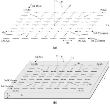
Consider a uniformly excited, rectangular, finite, planar, periodic array of (2N⫹ 1) ⫻ (2M ⫹ 1) dipoles. The array elements might be identical, short and thin, perfectly conducting wire dipole elements oriented along the x direction in the z⫽ 0 plane in air (free-standing dipoles), as illustrated in Figure 1(a), or identical printed dipoles on a grounded dielectric substrate with a thickness

d and relative dielectric constant⑀r, as depicted in Figure 1(b). For

both geometries, each dipole is assumed to have a length L and width W, and is uniformly spaced from its neighbors by distances

dxand dyin the x and y directions, respectively. The dipoles are

assumed to be center fed with infinitesimal generators.

2.1. The Method of Moments Solution

The dipoles are assumed to be thin (W Ⰶ L), so that only

xˆ-directed currents are required. Therefore, the current distribution

on each dipole is given by

Inm共 x⬘兲 ⫽ AnmPnm共 x⬘兲 fnm共 x⬘兲, (1)

where Anmis the unknown coefficient of fnm( x⬘) that determines

the current at the feed point on the element, and

Pnm共 x兲 ⫽

再

1 x僆 nmth_element

0 otherwise. (2) For the free-standing dipole array, the current fnm( x⬘) on the nmth

fnm共 x⬘兲 ⫽ sin

冋

k0

冉

L

2⫺ 兩x⬘ ⫺ ndx兩

冊册

(3)

where k₀is the free space wave number. Similarly, for the printed dipole array, the current fnm( x⬘) on the nmthdipole is expanded in

terms of piecewise sinusoidal (PWS) modes, defined as

fnm共 x⬘兲 ⫽ sin

冋

ka

冉

L 2⫺ 兩x⬘ ⫺ ndx兩

冊册

W sin

冉

ka L 2

冊

, (4)

where ka⫽ k0公(⑀r⫹ 1)/ 2 is the wavenumber of the expansion

mode.

An electric field integral equation (EFIE) is formed by enforc-ing the boundary condition, such that the total Exfield must vanish

on the dipole surfaces. This EFIE is solved using a Galerkin MoM solution, leading to the following set of linear equations:

Z៮ 䡠 I ⫽ V (5) where Z៮ ⫽ [Z_nm,pq], I⫽ [Anm], and V⫽ [Vpqe⫺jkx

pdx_e⫺jkyqdy_].

In Eq. (5), the right-hand side is related to the excitation at the pqth

dipole to radiate a direction beam according to (kx, ky), defined by

kx⫽ k0sin␪icos␾i; ky⫽ k0sin␪isin␾i, (6)

where (␪i,␾i) is the scan direction of the beam. Also, Znm,pqon

the left-hand side is the mutual impedance between the nmth_and

pqth_{dipoles, and is given by}

Znm,pq⫽ j␻␮

冕

Lpq

dx

冕

Lnm

dx⬘fpq共 x兲Gxx共rpq兩r⬘nm兲 fnm共x⬘兲 (7)

where rpq and r⬘nmare the position vectors of the pqthand nmth

dipoles and Gxx(rpq兩r⬘nm) is the corresponding component of the

(i) free-space dyadic Green’s function for the free-standing dipole array, and the (ii) planar microstrip dyadic Green’s function [16] for the printed dipole array.

Finally, note that for a scattering problem where an external plane wave is incident on the array, in which the elements are now passive, the right-hand side of Eq. (5) is associated with the incident field Ex i_(r pq), namely, Ex i 共rpq兲 ⫽ Vpqe⫺jkx pdx_e⫺jkyqdy␦共x ⫺ pd x兲. (8)

2.2. BiConjugate Gradient Stabilized Method (Bi-CGSTABM)

Bi-CGSTABM is a very reliable form of the conjugate gradient method (CGM) in terms of convergence. In this method, let Iibe

the value of I at the ith_{iteration with I}

0the initial guess. Then,

R₀⫽ V ⫺ Z៮ 䡠 I₀, S₀⫽ R₀. (9) At the ith_{iteration, the Bi-CGSTABM updates each vector in the}

following way: ␣i⫽ 具Ri, Ri典 具Z៮ 䡠 Si, Si典 , Ii⫹1⫽ Ii⫹␣iSi, Ri⫹1⫽ Ri⫺␣iZ៮ 䡠 Si (10) and ci⫽ 具Ri⫹1, Ri⫹1典 具Ri, Ri典 , Si⫹1⫽ Ri⫹1⫹ ciSi, (11)

where具, 典 denotes the inner product without complex conjugate. This procedure continues until a converged result is obtained. Details of this method can be found in [15].

3. ACCELERATION ALGORITHM BASED ON DFT EXPANSION

The repeated and time-consuming computations of Z៮ 䡠 I [I ⫽ I₀in Eq. (9) and I⫽ Siin Eq. (10)] type matrix-vector multiplications

in IMoM are accelerated using this DFT-based acceleration algo-rithm. In this algorithm, the contributing elements are divided into “strong” and “weak” interaction groups, as depicted in Figure 2(a), such that Z៮ 䡠 I ⫽

冘

nm僆strong AnmZnm,pq⫹

冘

nm僆weak AnmZnm,pq. (12)

The contributions coming from the strong interaction group are obtained via exact element-by-element computation and are the same for each receiving element. The size of the strong region is fixed and very small, compared to the entire array. Therefore, the computational complexity remains O(Ntot). Since the dominating

contributions are, in general, radiated from the strong group, the exact computation assures the fundamental accuracy of the method. On the other hand, the computation of contributions coming from the weak interaction group is based on a DFT expansion of the entire induced current on the array. Consequently, the contributions coming from the weak region to the pqth_element

is given by

Eweak共rpq兲 ⫽

冘

nm僆weak

AnmZnm,pq, (13)

Figure 1 Geometry of a periodic array of (2N⫹ 1) ⫻ (2M ⫹ 1) (a) free-standing dipoles and (b) printed dipoles

and by substituting the DFT representation [14] of Anm into Eq. (13), we obtain Eweak共rpq兲 ⫽

冘

k⫽⫺N N

冘

l⫽⫺M M Bkl ⫻

冘

nm僆weak Znm,pqe⫺jk xndx e⫺jkymdy e⫺j2␲共kn/ 2N⫹1兲e⫺j2␲共lm/ 2M⫹1兲, (14) where Bklis the coefficient of the klthDFT term and can be found

from the inverse DFT [14]. For a rectangular array, the significant DFT terms can be determined based on the criterion presented in [12], where the DFT terms of the orthogonal column (k⫽ 0) and row (l⫽ 0) dominate. However, considering the fact that contri-butions coming from the weak region provide minor corrections to the solution in contrast to the dominating strong group, very few significant DFT terms can be retained during the calculation of Eq. (14). Consequently, substituting (14) into (12) and keeping only the significant DFT terms, results in

Z៮ 䡠 I ⫽

冘

nm僆strong

AnmZnm,pq⫹

冘

kl僆Q

BklCkl,pq, (15)

where Q denotes the selected DFT terms, and

Ckl,pq⫽

冘

nm僆weak

Znm,pqe⫺jkx

ndx_e⫺jkymdy_e⫺j2␲共kn/ 2N⫹1兲_e⫺j2␲共lm/ 2M⫹1兲_{. (16)}

With this expression, only Q DFT terms (Q is a small, fixed number), which can be computed and stored before the Bi-CG-STABM proceeds, need to be computed for a given receiving element in addition to the contributions from the strong group. Consequently, O(Ntot) of computational complexity can be

ob-tained. Note that the coefficients of the DFT terms are initially obtained from the infinite array assumption, where only the central

element B₀₀is nonzero. Then, they are continuously updated at each iteration.

C_kl,pqin Eq. (16) denotes the contribution of the klth_{DFT term}

to the pqth_{receiving element, where each DFT term represents a}

linear phase impression. One way of fast computing C_kl,pqis to employ asymptotic techniques [12], which will decompose Eq. (16) in terms of few ray-like contributions due to edge and corner diffractions. However, in this paper, an alternative approach is employed which retains the computation complexity at O(Ntot). In

this approach, the weak group is also divided into “forward” and “backward” subgroups, where the “forward” group consists of elements in the front of the pqth_{receiving element, and the rest of}

the weak group elements are included in the “backward” group. It should be mentioned that the number of elements in these two groups varies according to the location of the pqth_{element, but the}

total number remains roughly the same for each receiving element. It is assumed that the iterative procedure sweeps elements in the order of⫺N ⱕ p ⱕ N, ⫺M ⱕ q ⱕ M (that is, pq ⫽ {11, 21, 31, . . . , 12, 22, . . . , 13, 23, . . .}). Then, one may find the contributions due to the “forward” subgroup C_kl,pqf

and the “back-ward” subgroup C_kl,pqb _{independently but iteratively. C}

kl,pqis only

their superposition. One may explain C_kl,pqf

in the following form:

Ckl,pq f ⫽

冘

mn僆W Znm,pqe⫺jkx ndx_e⫺jkymdy_e⫺j2␲共kn/ 2N⫹1兲_e⫺j2␲共lm/ 2M⫹1兲 ⫹

冘

n⫽⫺N N Zn共⫺M兲,pqe⫺jk xndx_e⫺jky共⫺M兲dy_e⫺j2␲共kn/ 2N⫹1兲_e⫺j2␲关l共⫺M兲/ 2M⫹1兴_, (17) where W is the “forward” when the (⫺M)th_{column [or 1}st_column

with respect to Fig. 1(a) or (b)] of the array is subtracted. Note that the mutual impedance Z_nm,pqdepends only on ( p⫺ n) and (q ⫺

m) for a periodic structure. As a result, the first term on the

right-hand side of Eq. (17) can be related to C_kl,p(qf _⫺1)

by Ckl,pq f ⫽ Ckl,pf 共q⫺1兲䡠 e⫺jkydye⫺j2␲共l/ 2M⫹1兲 ⫹

冘

n⫽⫺N N Zn共⫺M兲,pqe⫺jkxndxe⫺jky共⫺M兲dye⫺j2␲共kn/ 2N⫹1兲e⫺j2␲关l共⫺M兲/ 2M⫹1兴. (18) The details are illustrated in Figure 2(b). Basically, the forward weak group corresponding to the pqth_{receiving element [the solid}

loop in Figure 2(b)] is decomposed into two groups, as indicated by dotted and dashed loops. The dashed loop is identical to the dash-dotted loop, which is the forward weak group of p(q⫺ 1)th

receiving element, except a location shift which corresponds to a phase shift. It is noted that in the forward sweep Ckl,p(qf ⫺1) is

obtained before C_kl,pqf

is interested. The next step is the compu-tation of the second term in Eq. (18), namely,

Dkl,pq f ⫽

冘

n⫽⫺N N Zn共⫺M兲,pqe⫺jkxndxe⫺jky共⫺M兲dye⫺j2␲共kn/ 2N⫹1兲e⫺j2␲关l共⫺M兲/ 2M⫹1兴, (19) which contains the contributions coming from a one-dimensional (1D) array with the receiving element located far away from this array. Then, utilizing the dependence of Z_nm,pqon ( p⫺ n), Eq. (19) can be expressed as

Figure 2 (a) Decomposition of interaction elements in terms of strong and weak groups; (b) the forward weak group corresponding to the pqth

receiving element (the solid loop) is decomposed into two groups indicated by dotted and dashed loops. The dashed loop is identical to the dash-dotted loop, which is the forward weak group of p(q⫺ 1)th_{receiving element,}

Dkl,pq f _⫽

冘

n⫽⫺N⫹1 N Zn共⫺M兲,pqe⫺jkxndxe⫺jky共⫺M兲dye⫺j2␲共kn/ 2N⫹1兲e⫺j2␲关l共⫺M兲/ 2M⫹1兴 ⫹ Z共⫺N兲共⫺M兲,pqe⫺jkx共⫺N兲dxe⫺jky共⫺M兲dy ⫻ e⫺j2␲关k共⫺N兲/ 2N⫹1兴_e⫺j2␲关l共⫺M兲/ 2M⫹1兴 ₍₂₀₎

and the first term can be related to D_{kl,( p}f _⫺1)q

by Dkl,pq f ⫽ Dkl,f 共 p⫺1兲q䡠 e⫺jkxdxe⫺j2␲共k/ 2N⫹1兲 ⫺ ZN共⫺M兲,共 p⫺1兲qe⫺jkx共N⫹1兲dxe⫺jky共⫺M兲dye⫺j2␲关k共N⫹1兲/ 2N⫹1兴e⫺j2␲关l共⫺M兲/ 2M⫹1兴 ⫹ Z共⫺N兲共⫺M兲,pqe⫺jkx共⫺N兲dxe⫺jky共⫺M兲dye⫺j2␲关k共⫺N兲/ 2N⫹1兴e⫺j2␲关l共⫺M兲/ 2M⫹1兴. (21) Note that, if q is in the first few columns where the strong region occupies all contributing rows, special treatments must be em-ployed, even though the fundamental concepts are the same.

C_kl,pqb

, due to the “backward” group, can be found in a similar fashion by a backward sweep (that is, pq⫽ {NM, (N ⫺ 1) M, (N ⫺ 2) M, . . . , N(M ⫺ 1), (N ⫺ 1)(M ⫺ 1), . . .}). Indeed, the formulation is identical to (17)–(21), except that the multipli-cation “䡠 ” is replaced by division “/”.

The storage and complexity requirements of this algorithm are as follows: (a) storage of the unknown current vector in the iterative process is Ntot; (b) storage of DFT terms is Q, where Q

Ⰶ Ntot and is fixed regardless of the array size; (c) storage of C_kl,pq is Q ⫻ Ntot; (d) the complexity of the strong region of

computation is Ns⫻ Ntot, where NsⰆ Ntotand Ns, the size of the

strong region, is fixed regardless of the array size; (e) the com-plexity of the weak region of computation is Q⫻ Ntot; (f) finally,

the total complexity for the computations of C_kl,pqand D_kl,pqis 2Q⫻ Ntot, consequently, the total cost is O(Ntot).

4. NUMERICAL RESULTS

In this section, the accuracy and efficiency of the proposed method are investigated. Numerical results for both free-standing and printed dipole arrays are obtained using this IMoM method with the DFT-based acceleration algorithm, and compared with the results obtained via conventional MoM. In all examples, the arrays are excited uniformly in amplitude so that Vpq⫽ 1 in Eq. (5) for

each pqth_dipoles.

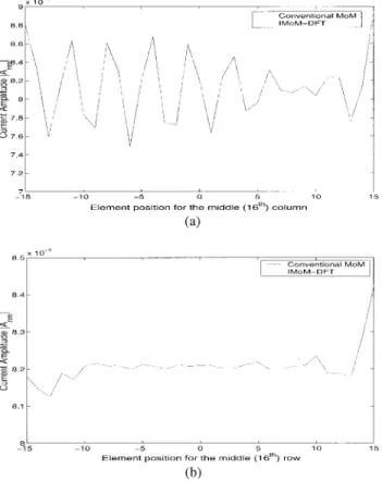
In Figure 3(a) and (b), magnitude of the current distribution ( Anm) of the middle column (16thcolumn, m⫽ 0) and middle row

(16th_{row, n⫽ 0) versus element position pertaining to a 31 ⫻ 31}

free-standing dipole array with dx⫽ 0.6␭0and dy⫽ 0.3␭0(with

␭0the free-space wavelength) are shown. The length and the radius

of each dipole is 0.4␭₀and 0.0005␭₀, respectively. The elements are phased to radiate a beam maximum in the direction of (␪ ⫽ 20°,␾ ⫽ 10°). For this example, 15 DFT terms are selected (Q ⫽ 15) and the size of the strong region is 3⫻ 3 (Ns⫽ 9) with the

receiving element being located at the center of the strong region. The results obtained from IMoM-DFT agree well with the refer-enced results.

As for the printed dipoles, Figure 4(a) and (b) depicts the magnitude of the current distribution ( Anm) of the middle (21st

column, m⫽ 0) and last (41st_{column, m⫽ 20) columns versus}

Figure 3 Comparison of the magnitude of induced current兩Anm兩 ob-tained via IMoM-DFT and conventional MoM for the (a) middle (16th₎

column (n ⫽ ⫺15 : 15 and m ⫽ 0); (b) middle (16th_{) row (m ⫽}

⫺15 : 15 and n ⫽ 0)

Figure 4 Comparison of the magnitude of induced current兩Anm兩 ob-tained via IMoM-DFT and conventional MoM for the (a) middle (21st₎

column (n ⫽ ⫺20 : 20 and m ⫽ 0); (b) last (41st_{) column (n ⫽}

element position, pertaining to a 41⫻ 41 printed dipole array with

dx⫽ dy⫽ 0.5␭0. The slab has a thickness of 0.05␭0(relatively

thin) and its relative permittivity is⑀r ⫽ 2.55. The length and

width of each dipole is 0.39␭₀ and 0.01␭₀, respectively, and the elements are phased to radiate a beam maximum in the direction of (␪ ⫽ 30°, ␾ ⫽ 40°). Overall, five DFT terms with a strong region of 3⫻ 3 are used. Very good agreement between IMoM-DFT and conventional MoM is obtained, as illustrated by these results.

In a similar way, a 31⫻ 31 printed dipole array with the same parameters for each element is investigated for a thicker substrate

d⫽ 0.19␭₀ with the same⑀r⫽ 2.55. The comparison between

the IMoM-DFT and conventional MoM of the magnitude of the current distribution ( Anm) of the 2nd(m⫽ ⫺14) and 13th(m⫽

⫺3) are illustrated in Figure 5(a) and (b) for a broadside scan case (␪ ⫽ 0°, ␾ ⫽ 0°). Again, fairly good agreement is obtained. The only problem is that, regardless of the size of the array, as the thickness of the substrate increases due to the surface waves, more DFT terms (or a slight increase in the strong region) may be required. Therefore, in this example Q⫽ 21, although the strong region has still the same size (3⫻ 3). Nevertheless, this is a case where FBM accelerated with a DFT-based algorithm has conver-gence problems, which are probably due to the nature of FBM, as claimed in [9].

Finally, the radiation pattern (E_␪) of a 21⫻ 21 printed dipole array, with dx ⫽ dy⫽ 0.5␭0, d ⫽ 0.05␭0, and ⑀r ⫽ 2.55 is

obtained with IMoM-DFT and compared with the result of the conventional MoM in Figure 6. The length and the width of each element is ldip ⫽ 0.39␭0 and wdip ⫽ 0.01␭0, respectively, and

elements are phased to radiate a beam maximum in the direction of

(␪ ⫽ 30°, ␾ ⫽ 40°). Agreement with the referenced result is again very good, thereby establishing confidence in the present IMoM-DFT approach.

5. DISCUSSION AND CONCLUSION

An efficient and accurate analysis method for radiation/scattering from electrically large phased arrays of both free-standing and printed dipoles is presented. Both the computational complexity and the memory storage of the IMoM solution are reduced to

O(Ntot) by using a DFT-based acceleration algorithm. Numerical

results demonstrate the efficiency and accuracy of this method. The present approach will be extended to treat finite arrays with tapered excitations and non-rectangular array shapes. It should be noted that the contributions from DFT terms can also be efficiently found by asymptotic techniques [12], in terms of ray solutions. Consequently, they can be incorporated into ray-tracing codes to account for the interactions between the array and the environ-ment.

REFERENCES

1. R.F. Harrington, Field computation by moment methods, IEEE Press, New York, 1993.

2. N. Engheta, W.D. Murphy, V. Rokhlin, and M.S. Vassiliou, The fast multipole method (FMM) for electromagnetic scattering problems, IEEE Trans Antennas Propagat 40 (1992), 634 – 641.

3. R.J. Burkholder and D.H. Kwon, High frequency asymptotic acceler-ation of the fast multipole method, Radio Sci 31 (1996), 1199 –1206. 4. X.Q. Sheng, J.-M. Jin, J. Song, W.C. Chew, and C.-C. Lu, Solution of combined-field integral equation using multilevel fast multipole algo-rithm for scattering by homogeneous bodies, IEEE Trans Antennas Propagat 46 (1998), 1718 –1726.

5. Y. Zhuang, K.-L. Wu, C. Wu, and J. Litva, A combined full-wave CG-FFT method for rigorous analysis of large microstrip antenna arrays, IEEE Trans Antennas Propagat 44 (1996), 102–109. 6. H.-T. Chou, Extension of the forward-backward method using spectral

acceleration for the fast analysis of large array problems, IEE Proc Microwave Antennas Propagat 147 (2000), 167–172.

7. H.-T. Chou and H.-K. Ho, Implementation of a forward-backward procedure for the fast analysis of electromagnetic radiation/scattering from two dimensional large phased arrays, IEEE Trans Antennas Propagat (submitted).

8. O¨ .A. Civi, Extension of forward backward method with DFT based acceleration algorithm for the efficient analysis of large printed dipole Figure 5 Comparison of the magnitude of induced current兩Anm兩

ob-tained via IMoM-DFT and conventional MoM for the (a) 2nd_{column (n⫽}

⫺15 : 15 and m ⫽ ⫺14); (b) 13th_{column (n⫽ ⫺15 : 15 and m ⫽ ⫺3)}

Figure 6 Far-field pattern of a 21⫻ 21 printed dipole array radiate a beam maximum in the direction of (␪ ⫽ 30°, ␾ ⫽ 40°)

arrays, 2002 IEEE AP-S Int Symp Antennas Propagat and USNC/ URSI Natl Radio Sci Mtg, San Antonio, TX, 626 – 629.

9. O¨ .A. Civi, Extension of forward-backward method with a DFT-based acceleration algorithm for efficient analysis of radiation/scattering from large finite-printed dipole arrays, Microwave Opt Technol Lett 37 (2003), 626 – 629.

10. V.B. Ertu¨rk and H.T. Chou, Fast acceleration algorithm based on DFT expansion for the iterative MoM analysis of electromagnetic radiation/ scattering from two-dimensional large phased arrays, 2002 IEEE AP-S Int Symp Antennas Propagat and USNC/URSI Natl Radio Sci Mtg, San Antonio, TX, 156 –159.

11. O¨ .A. Civi, P.H. Pathak, H.-T. Chou, and P. Nepa, A hybrid uniform geometrical theory of diffraction-moment method for the efficient analysis of electromagnetic radiation/scattering from large finite planar arrays, Radio Sci 35 (2000), 607– 620.

12. H.-T. Chou, H.-K. Ho, P.H. Pathak, P. Nepa, and O¨ .A. Civi, Efficient hybrid discrete Fourier transform-moment method for fast analysis of large rectangular arrays, IEE Proc Microwave Antennas Propagat 149 (2002), 1– 6.

13. A.K. Skrivervik and J.R. Mosig, Finite phased array of microstrip patch antennas: The infinite array approach, IEEE Trans Antennas Propagat 40 (1992), 579 –582.

14. A.V. Oppenheim and R.W. Schafer, Discrete-time signal processing, Prentice Hall, New York, 1999.

15. T.K. Sarkar, On the applications of generalized biconjugate gradient method, J Electromagn Wave Appl 1 (1987), 223–242.

16. S. Barkeshli, P.H. Pathak, and M. Marin, An asymptotic closed-form microstrip surface Green’s function for the efficient moment method analysis of mutual coupling in microstrip antennas, IEEE Trans An-tennas Propagat 38 (1990), 1374 –1383.

© 2003 Wiley Periodicals, Inc.

LOSSY EFFECTS ON THE TRANSIENT

PROPAGATION IN LTCC COPLANAR

WAVEGUIDES (CPWS)

W. Y. Yin, B. Guo, X. T. Dong, and Y. B. Gan Temasek Laboratories

National University of Singapore Singapore 119260

Received 17 March 2003

ABSTRACT: The effects of dielectric, radiative leakage and ohmic

losses in CPWs on the propagation of Gaussian and sinusoidally modu-lated Gaussian pulses are investigated. These CPWs are assumed to be fabricated on a single-layer low-temperature co-fired ceramic (LTCC) substrate. It is shown that, based on the improved empirical formula for accurate prediction of the ohmic attenuation constant presented by Liao et al., the lossy effects in LTCC CPWs are dominated by the ohmic loss of the center and ground conductive planes in the frequency range up to 40 GHz. © 2003 Wiley Periodicals, Inc. Microwave Opt Technol

Lett 39: 94 –97, 2003; Published online in Wiley InterScience (www. interscience.wiley.com). DOI 10.1002/mop.11137

Key words: coplanar waveguides (CPWs); LTCCs; ohmic loss; pulse

wave; attenuation

1. INTRODUCTION

The conductor losses of coplanar waveguides (CPWs) have been studied by many researchers using different techniques [1–9]. Physically, as the operating frequency increases, the dielectric loss, radiation loss, and ohmic loss of CPWs have significant effects on the pulse-waveform distortion [7, 8]. In particular, Liao and Pon-chak et al. have presented two sets of new empirical formulas to

predict the ohmic loss for CPWs [8, 9], respectively, which are characterized by different conductivities and thicknesses of the center strip and ground planes over a wideband frequency range. In this work, we focus on different lossy effects of low-temperature co-fired ceramic (LTCC) CPWs on the transient char-acteristics of Gaussian or sinusoidally modulated Gaussian pulse propagation. Because LTCCs have excellent high-frequency per-formances, they have been widely used as substrates or super-strates in high-density interconnects and packaging systems [10, 11]. This paper is organized as follows: in section 2, the geometry of a LTCC CPW is shown, and some formulas to determine the dielectric loss, radiation leakage loss and ohmic loss are intro-duced. Based on these formulas and the fast Fourier transformation (FFT), in section 3, the transient propagated pulses are computed and compared, for different LTCC substrates and center strip and ground plane thicknesses, and their conductivities. Some conclu-sions of this work is presented in section 4.

2. GEOMETRY

The geometry of an LTCC CPW is shown in Figure 1, with LTCC thickness D, center strip width is W, and strip spacing S. Physi-cally, the permittivity and loss tangent of LTCCs can be chosen as (␧r, tan␦) ⫽ (4.2, 0.003), (5.9, 0.002), (7.0, 0.002), (7.8, 0.0015),

(8.2, 0.002), and (10.6, 0.001), respectively. The thickness and conductivity of the center strip and ground plane are characterized by t and␴, respectively.

Mathematically, the attenuation constant that results from the dielectric loss of the LTCC substrate can be evaluated by [5]:

␣d⫽ 0.3145 ␧r

冑

␧re共 f 兲 ␧re共 f 兲 ⫺ 1 ␧r⫺ 1 tan␦ ␭0 共Np/unit length兲, (1)

where␧re( f ) is the effective dielectric constant of the CPW, and

can be accurately determined by some empirical formulas; f is the operating frequency, and␭₀is the wavelength in free space. The attenuation constant of the CPW at high frequency due to the radiative leakage can be determined by [5, 8]:

␣r共 f 兲 ⫽ 2

冉

␲ 2

冊

5

冦

冋

1⫺␧re共 f 兲 ␧r

册

2

冑

␧re共 f 兲 ␧r

冧

共w ⫹ 2s兲2_␧ r 3/ 2 c3_{K⬘共k兲 K共k兲} f3 共Np/unit length兲, (2) where k ⫽ w/(w ⫹ 2s), and K(k) and K⬘(k) are the complete elliptic integrals of the first and second kinds, respectively. The attenuation constant of the CPW due to ohmic loss can be evalu-ated by [5]:

Figure 1 Geometry of an LTCC CPW: (a) three-dimensional view; (b) cross-sectional view