Selçuk J. Appl. Math. Selçuk Journal of Vol. 8. No.1. pp. 27-43 , 2007 Applied Mathematics
Control of a Double-Inverted Pendulum For Nonlinear System Mustafa Demirci
Gaziosmanpasa University Tokat Occupational School Tasliciftlik Campus, 60100 Tokat, Turkey
e-mail:m dem irci34@ yahoo.com
Received : December 25, 2006
Summary. The aim of the paper is to compare two different techniques to design a stabilizing control the double inverted pendulum in an upright posi-tion. These techniques are the Pole Placement and Linear Quadratic Regulator. Techniques have been used to design controls for the nonlinear system. For our double pendulum system, it would be desirable to keep the values of the state variables small as a large displacement from the origin may cause the nonlinear system to be unstable we would also interested in the control that gives the largest region of stability for the system, as we then could allow a larger set of perturbations from upright position.
Key words:Nonlinear , Stability, Pole Placement,Linear Quadratic Regulator and Double-Inverted Pendulum
1. Introduction
To design a stabilizing controller for a single inverted pendulum is a typical problem in control system design based on the state space approach [1] [2] and is known as a good analogy to the design of a controller for launching a rocket. A stabilize pendulum is useful to show the power of a control mechanism to laymen of the state space theory.
This paper follows up work carried out in a recent publication [10] by the same author, who dealt with the design of feedback controllers for linear system with applications to control of a double-inverted pendulum. Previously, the problem of stabilizing the double inverted pendulum for the linear system had been solved using two different techniques that were the Pole Placement and Linear Quadratic Regulator to design for the system.
The current paper focuses on the nonlinear system, to compare same techniques to design a stabilizing controller for the double inverted pendulum in an upright position. The pendulum system we will investigate is based on the system
described in [3] with the assumptions that the double inverted pendulum moves on a horizontal rail.
2.Mathematical Model for Double Inverted Pendulum
The pendulum system we will take the double inverted pendulum as described in [3] with the assumption. The double inverted pendulum moves on a horizontal rail is schematically shown in Figure 1. The system is composed of:
A double inverted pendulum consisting of two aluminum rods, which are con-nected by a hinge, and the lower rod concon-nected to a cart by a second hinge. The motion of the rods is smooth and is restricted to the vertical plane containing the double pendulum.
·A cart moves on a horizontal rain.
·The cart-driving system consisting of a motor, a pulley and belt transmission system using a timing belt and power amplifier.
Figure.1.Diagram of the Double Inverted Pendulum System
Some assumptions were given by Furute et al (1978) in the mathematical model of the system.
·Each pendulum is rigid body
·The length of the belt does not change during the experiment.
·The driving force to the cart is directly applied to the cart without delay and is proportional to the input to the amplifier.
·The friction force against the motion of the cart, and frictional force generated at the connecting hinges is proportional to the difference the angular velocities of the upper and lower pendulums.
The above assumptions were given by Furute et al. A mathematical model can be derived on the Lagrange equation according to the above assumptions. But
the kinetic energy, potential energy and dissipation energy will be given here for our case of the motion of the double inverted pendulum on a horizontal rail, assuming that subscripts 1 and 2 denote the lower and upper pendulums respectively.
(1) For the Lower Pendulum: Kinetic Energy 1= 1 21˙ 2 1+ 1 21 (∙ (1sin 1) ¸2 + ∙ (1cos 1) ¸2) Potential Energy 1= 11cos 1 Dissipation Energy 1= 1 21˙ 2 1
(2) For the upper pendulum: Kinetic Energy 2= 1 22˙ 2 2+ 1 22 (∙ ( sin 1+ 2sin 2) ¸2 + ∙ ( cos 1+ 2cos 2) ¸2) Potential Energy 2= 2( cos 1+ 2cos 2) Dissipation Energy 2= 1 21 ³ ˙21+ ˙22´ (3) For the cart:
Kinetic Energy 3= 1 2 ˙ 2 Potential Energy 3= 0 Dissipation Energy 3= 1 2 ˙ 2
where r is the distance of the cart from the reference position, 12 are the
m denote the mass, l the distance between the center of the hinge and its
center of gravity, J is moment of inertia and c is the friction coefficient for
rotation between the pendulum and hinge. L is the length (between the hinges) of the lower pendulum. M, F are the mass and friction coefficients of the cart and g is the acceleration of gravity.
= 3 X =1 = 3 X =1 = 3 X =1
Then the following relations exist (summing the kinetic, potential and dissipa-tion energies) µ ˙ ¶ − + + = (1) µ ˙ ¶ − + + ˙ = 0 = 1 2
where is the gain of overall cart driving system and e is the input to voltage to the amplifier satisfying 0> ||.
¯ = [ 1 2] 0= and (1) is writtenas 1¯00= 2¯0+ 3+ 4 where 1= ¯ ¯ ¯ ¯ ¯ ¯ 1+ 2+ (11+ 2) cos 1 22cos 2 (11+ 2) cos 1 1+ 112+ 22 22 cos (1− 2) 22cos 2 22 cos (1− 2) 2+ 222 ¯ ¯ ¯ ¯ ¯ ¯ 2= ¯ ¯ ¯ ¯ ¯ ¯ − (11+ 2) ˙1sin 1 22˙2sin 2 0 −1− 2 −22 ˙2sin (1− 2) + 2 0 −22 ˙1sin (1− 2) + 2 2 ¯ ¯ ¯ ¯ ¯ ¯ 3= ¯ ¯ ¯ ¯ ¯ ¯ 0 (11+ 2) sin 1 22 sin 2 ¯ ¯ ¯ ¯ ¯ ¯ 4= ¯ ¯ ¯ ¯ ¯ ¯ 0 0 0 ¯ ¯ ¯ ¯ ¯ ¯ Now we define = ¯ ¯ ¯ ¯ _ _ 0 ¯ ¯ ¯ ¯ Then
0= ¯ ¯ ¯ ¯ ¯ _ 0 1−1³2 _ 0+ 3+ 4 ´ ¯ ¯ ¯ ¯ ¯
gives the mathematical model for the double inverted pendulum system, where ˙ = 0.
To analyze non-linear systems is much difficult than linear systems. One of the principal techniques for the analysis of nonlinear systems is to approximate or bound them by appropriate linear systems, and then use linear theory. The nonlinear case is different in two essential respects. First, since equilibrium points are solutions, in this case, to nonlinear equations, finding such solutions is somewhat more of an accomplishment than in the linear case. Thus, a de-scription of equilibrium points often constituter significant information. Second, and perhaps more fundamentally, the equilibrium point distribution points in virtually any special pattern in state space.
3.Stability
We consider the nonlinear system ˙ = () where is continuously differentiable function.
Definition 1: ˙ = () has an equilibrium at ¯ so that (¯) = 0.
Definition 2: The equilibrium is stable if, given any 0, there exists 0 such that |(0) − ¯| implies |() − ¯| for all 0.
Definition 3: ¯ is an asymptotically stable equilibrium point if it is stable and convergent. : If there exists ∆ 0 such that |(0) − ¯| ∆ implies that () → ¯ as → ∞ .
Definition 4: ¯ is an unstable equilibrium point if it is not stable
Definition 5:Let us consider a nonlinear system such as ˙ = () and expand it into the form ˙ = () + () where () contains all the higher powers of to the extent that
lim
kk→0=
k()k kk = 0
() goes to zero faster than does. Liapunov has shown that such a system will be stable if all the eigenvalues of are strictly inside the left hand part. Now, let ˙ = (), (0) = 0 and ¯ equilibrium point then we can write
˙ = (¯) + ( − ¯) + ( − ¯)
where ∈ <and represents higher powers of ( − ¯) If Definition 5 is used,
lim
k−¯k→0=
k ( − ¯)k k − ¯k = 0
Hence ( − ¯) → 0 faster than ( − ¯) → 0 and so the higher powers in ( − ¯) can be neglected,
() − (¯) = ( − ¯) ˙ − ˙¯ = ( − ¯) If we recall 0= − ¯ , we get
˙0 = 0 0(0) = 0− ¯
the linearisation of the nonlinear system.
According to Liapunov’s first method, which says that the linearized system is asymptotically stable at the origin, ¯ is asymptotically stable for the nonlinear system.
We now consider the control system ˙ = ( ), we have the conditions that is (¯ ) = 0 and the equilibrium point of the system is (¯ 0) .If we expand as before, we have
˙ = (¯ 0) + ( − ¯) + + ( − ¯ )
we can ignore the higher powers as before and the linearization of the nonlinear controlled system is
(2) ˙0= 0+ 0(0) = 0− ¯
If we return to Liapunov’s first method, we have to get a system as ˙0 = 0
where is system matrix. If is taken as 0 and substituting into (2), we get
(3) ˙0 = 0+ 0
˙0= ( + )0 0(0) = 0− ¯
where (A+BF) is system matrix and we can say that the linearization of the controlled system (3) approximates the nonlinear system at the point ¯. The nonlinear system can be thought of a perturbation of the linear system. If we can take a linear system of the form given by (3) and there is a feedback con-trol, which brings the system back to the upright position, the same control will also work in the nonlinear case for small perturbations around the equilibrium position. = ∙ 0 3 −11 30 −11 2 ¸ = ∙ 0 −11 4 ¸
03= ¯ ¯ ¯ ¯ ¯ ¯ 0 0 0 0 (11+ 2) 0 0 0 22 ¯ ¯ ¯ ¯ ¯ ¯ 4= ¯ ¯ ¯ ¯ ¯ ¯ 0 0 0 ¯ ¯ ¯ ¯ ¯ ¯ 1|1=2=0= ⎡ ⎣ 11+ 1+ 2+ 2 1+ 111+ 12+ 222 2222 22 22 2+ 222 ⎤ ⎦ 2|1=2= ˙1= ˙2=0= ⎡ ⎣ −0 −10− 2 02 0 2 −2 ⎤ ⎦
For the analysis and synthesis of a control system the following equivalent system is used
˙ = + = = [30]
where 3 is the 3x3 identity matrix, the vector is the state, the 3-vector y is
the output and the scalar is the input of the system. [ : ] = ¯ ¯ ¯ ¯ 021 223 ¯ ¯ ¯ ¯ 02 ¯ ¯ ¯ ¯ where 21= −11 3 22= 1−12 2= −11 4.
Thus a mathematical model of the double inverted pendulum has been derived. Since parameters have been given by Furuta et al, we will take those numerical values in order to simulate the double pendulum system. Parameters that are given in Table 1:
By substituting all parameters in the linearised model of the system we have 21 = ¯ ¯ ¯ ¯ ¯ ¯ 0 −23318 00672 0 483079 −132645 0 −532131 491599 ¯ ¯ ¯ ¯ ¯ ¯ 22= ¯ ¯ ¯ ¯ ¯ ¯ −46810 00140 −00048 134514 −03765 01861 −15558 06688 −04591 ¯ ¯ ¯ ¯ ¯ ¯ 2 = ¯ ¯ ¯ ¯ ¯ ¯ 230889 −670654 77568 ¯ ¯ ¯ ¯ ¯ ¯
Since the eigenvalues of the matrix A are
[0 82299 45047 −93104 −56993 −31914]
We have two positive eigenvalues and one zero eigenvalue. Therefore, the system is unstable.
The system is contrable, because of the rank of the matrix is equal 6 to for the double pendulum system. Hence, we have that the double inverted pendulum system is controllable and observable. Therefore we are able to stabilize the system and design a dynamic observer for the system.
Full details of Feedback Control, Dynamical Observers, the Pole Placement and the Linear Quadratic Regulator are given in [10].
4.Nonlinear System
Euler’s method will be used to solve the nonlinear system for approximating the differential equation ˙ = ( ) then an approximation solution to this equation is found as follows:
(+1) = () + ∆ (()) = 1 2 3
where (0) = 0and ∆ = +1− is the step size.
5.Nonlinear
This solves for the nonlinear system with feedback = − , and intial condition is 0: ˙ = 0 ¯0=h˙ ˙1 ˙2 i 0= ¯ ¯ ¯ ¯ ¯ _ 0 1−1³2 _ 0+ 3+ 4 ´ ¯ ¯ ¯ ¯ ¯ 6.Nonlinear-observer
() is the state and ˆ is the observer we will solve two equations: 0= ¯ ¯ ¯ ¯ ¯ _ 0 1−1³2 _ 0+ 3+ 4 ´ ¯ ¯ ¯ ¯ ¯ ˙ˆ = + ( − − )ˆ where = ˆ 7.Nonlinear-observer error
We will solve two equations to get the error of the observer varies with time:
0= ¯ ¯ ¯ ¯ ¯ _ 0 1−1³2 _ 0+ 3+ 4 ´ ¯ ¯ ¯ ¯ ¯ where = ( + ) ˙ = ( − )
This equation expresses the error dynamics ˙ of the estimate in terms of the system matrix , the measurement matrix and the observer matrix . We see that if is chosen so that ( − ) is a stable system matrix then tends to zero. Indeed, the error tends to zero at a rate determined by the dominant eigenvalue of ( − ). The eigenvalues of this matrix are controlled by our choice of the matrix .
8.Results for the Pole Placement Technique
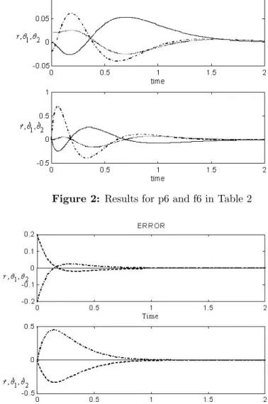
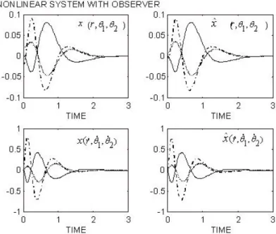
The best control found by this technique was p6. The graph in Figure 2 shows the behavior of the nonlinear system with the control p6. Figure 3 shows the graph of G4, the control G4 had the largest radius of stability.
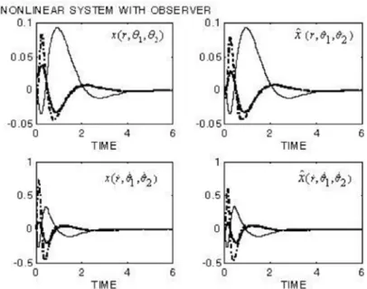
Figure 4 and 5 show the resulting behavior for the nonlinear systems with the observer.
9.The Linear Quadratic Regulator Method
The first control designed using this method used the matrix
= {0001 10 10 0001 0001} the weight the state variables.
Experience gained in using the pole placement method showed that if were not controlled heavily, the system would then take a long time to damp. Inves-tigation then continued to see how large the penalty on ˙ 1 2 should be. It
was noticed that this method seems to minimize the oscillatory behavior of the system.
As has been shown in the graphs for the pole placement technique [10], the behavior of the linearsied system is extremely close to that of the nonlinear system for the small initial condition that was chosen. Therefore only the graphs that concern the nonlinear system are shown, in Figure 6,7,8 and 9.
10.Conclusion
Euler’s method has been used to solve the nonlinear system. The main disad-vantage with the Euler algorithm is the fixed integration step size ∆. Size of the step affects the degree of accuracy and also the stability properties of the calculated solution.
A smaller step size requires more calculation to be performed over the same time interval and so increases the time taken to computer solutions. Obviously, a step size must be chosen which minimizes the time for computation while providing an accurate behavior of the actual system. Typical step sizes used in the simulations were of the order of 10−2 or 10−3 seconds. Any smaller step
size would result in a much longer run-time for the algorithms. Unfortunately, this means that the results may not be extremely accurate.
To design controls by the pole placement technique generate very small regions of stability for the nonlinear system and observer. Therefore the pole placement technique gave the least satisfactory results. The nonlinear model shows that the system is complicated and likely to be sensitive to small disturbance.
In this part, some graphs will be given which are simulations of the pendulum system and Table 6 is given which is the key for the graphs.
Figure 2: Results for p6 and f6 in Table 2
Figure 4: Results for p6 and G4 in Table 2 and 3
Figure 6: Results for LQ3 in Table 4
Figure 8: Results for LG3 and LQ3 in Table 4 and 5
References
1. Bryson, A. E., Jr., and Luenberger, D. G., 1970, Proc. Inst. Elect. Electron. Engrs, 58, 1803.
2.Mori, S., Nishihara, H., and Furuta, K., 1976 Int. J. Control, 23, 673.
3.Furuta, K., Kajiwara, H., and Kosuge, K., 1980 Int. J. Control, Vol.32, No.5, 925. 4.Friedland, B. Control System Design, McGraw-Hill, Inc. 1986.
5.Richards, R., J., An Introduction to Dynamics and Control. Longman 1979 6.Franklin, G., F., Powell, J., D., Emami-Naeini, A., Feedback Control of Dynamics Systems. 3 ed. Addison-Wesley Publishing Company, Inc.1994.
7. DiStefano, J., J., Stubberud, A., R., Williams, I., J., Feedback and Control. McGraw-Hill, Inc. 1995.
8. Luenberger, D., G., Introduction to Dynamical Systems, Theory, Models and Ap-plications. John Wiley&Sons, Inc. 1979.
9. Frederick, K., Chow, H., Feedback Control Problems Using MATLAB and The Control System Toolbox, PWS publishing Company. 1995.
10. Mustafa Demirci “Design of Feedback Controllers for Linear System with Appli-cations to Control of a Double-Inverted Pendulum”. Int. Journal of Computational Cognition, Volume 2, No 4, Pages 65-84, December 2004.