3D RECONSTRUCTION USING A SPHERICAL
SPIRAL SCAN CAMERA
A Thesis Submitted to
the Graduate School of Engineering and Sciences of
zmir Institute of Technology
in Partial Fulfillment of the Requirements for the Degree of
MASTER OF SCIENCE
in Computer Engineering
by
Mustafa VATANSEVER
October 2006
ZM R
We approve the thesis of Mustafa VATANSEVER
Date of Signature
. . . 10 October 2006 Prof. Dr. Sıtkı AYTAÇ
Supervisor
Department of Computer Engineering zmir Institute of Technology
. . . 10 October 2006 Asst. Prof. Dr. evket GÜMÜ TEK N
Co-Supervisor
Department of Electrical and Electronics Engineering zmir Institute of Technology
. . . 10 October 2006 Prof. Dr. Halis PÜSKÜLCÜ
Department of Computer Engineering zmir Institute of Technology
. . . 10 October 2006 Asst. Prof. Dr. Zekeriya TÜFEKÇ
Department of Electrical and Electronics Engineering zmir Institute of Technology
. . . 10 October 2006 Prof. Dr. Erol UYAR
Department of Mechanical Engineering Dokuz Eylül University
. . . 10 October 2006 Prof. Dr. Kayhan ERC YE
Head of Department
Department of Computer Engineering zmir Institute of Technology
. . .
ACKNOWLEDGEMENTS
I would like to thank to my supervisor Prof. Dr. Sıtkı Aytaç for his guidance and support. I would like to thank to my co-supervisor Asst. Prof. Dr. evket Gümü tekin for his guidance, ideas and invaluable support on solving the technical details.
I also would like to thank to Prof. Dr. Halis Püskülcü, Asst. Prof. Dr. Zekeriya Tüfekçi, Prof. Dr. Erol Uyar and Inst. Tolga Ayav for their advice in revising the thesis.
ABSTRACT
3D RECONSTRUCTION USING A SPHERICAL SPIRAL SCAN
CAMERA
Construction of 3D models representing industrial products/objects is commonly used as a preliminary step of production process. These models are represented by a set of points which can be combined by planar patches (i.e. triangulation) or by smooth surface approximtions. In some cases, we may need to construct the 3D models of real objects. This problem is known as the 3D reconstruction problem which is one of the most important problems in the field of computer vision.
In this thesis, a sytem has been developed to transform images of real objects into their 3D models automatically. The system consists of a PC, an inexpensive camera and an electromechanical component. The camera attached to this component moves around the object over a spiral trajectory and observes it from different view angles. At the same time, feature points of object surface are tracked using a tracking algorithm over object images. Then tracked points are reconstructed in 3D space using a stereo vision technique. A surface approximation is fitted to this 3D point set as a last step in the process. Open source “Intel®-OpenCV” C library is used both in image capturing and in image processing.
ÖZET
KÜRESEL SP RAL TARAYICI KAMERA LE 3B GER ÇATIM
Endüstriyel ürünlerin/nesnelerin 3B modellerinin olu turulması genellikle üretim sürecinin ilk adımı olarak kullanılmaktadır. Bu modeller noktalar kümesiyle gösterilir ve bu noktalar üçgen gibi düzlemsel elemanlarla veya düzgün yüzey yakla ımlarıyla birle tirilir. Ancak bazı durumlarda gerçek nesnelerin 3B modellerini olu turmamız gerekebilir. Bu problem 3B geriçatım problemi olarak bilinir ki; bu problem bilgisayarla görme alanının en önemli problemlerinden biridir.Bu tezde gerçek nesnelerin görüntülerinden 3B modellerine otomatik geçi i sa layan bir 3B geriçatım sistem geli tirilmi tir. Sözkonusu sistem bir PC, dü ük maliyetli bir kamera ve elektromekanik bir parçadan olu maktadır. Elektromekanik parçaya ba lı kamera nesne etrafında spiral bir yörüngede hareket ettirilerek nesneyi de i ik açılardan görmesi sa lanmı tır. Aynı zamanda bir takip algoritmasıyla, nesne yüzeyinde belirleyici niteli i olan noktaların, nesne görüntüleri üzerindeki takibi yapılmı tır. Bir “ikili görme” tekni i kullanılarak takip edilen noktaların 3B geriçatımı yapılmı tır. Son adım olarak geriçatımı yapılmı olan 3B nokta kümesinden bir yüzey yakla ımı elde edilmi tir. Kameradan görüntü alımı ve i lenmesinde açık kaynak kodlu “Intel®-OpenCV” C kütüphanesi kullanılmı tır.
TABLE OF CONTENTS
LIST OF FIGURES ... vii
CHAPTER 1. INTRODUCTION... 1
CHAPTER 2. CAMERA CALIBRATION... 4
2.1. Pinhole Camera Model (Perspective Projection Model) ... 4
2.2. Intrinsic Camera Calibration... 6
2.2.1. Intrinsic Camera Calibration Using Matlab Camera Calibration Toolbox ... 9
2.3. Extrinsic Camera Calibration... 10
CHAPTER 3. 3D RECONSTRUCTION FROM MULTIPLE VIEWS ... 14
3.1. Single View Geometry... 14
3.2. Two View Geometry (Stereo Visio)... 15
CHAPTER 4. EXPERIMENTAL SETUP: SPHERICAL SPIRAL SCAN MECHANISM ... 17
4.1. Stepper Motors... 21
CHAPTER 5. 3D RECONSTRUCTION ALGORITHM ... 24
5.1. Feature Point Detection ... 27
5.2. Tracking of Feature Points... 30
5.3. 3D Reconstruction of Tracked Feature Points... 35
CHAPTER 6. SURFACE FITTING ... 42
CHAPTER 7. CONCLUSIONS... 46
LIST OF FIGURES
Figure
Page
Figure 1.1. General system setup illustration... 2
Figure 2.1. Pinhole camera model... 4
Figure 2.2. Side view of pinhole camera model... 5
Figure 2.3. Scaling factor ... 6
Figure 2.4. Scew factor ... 7
Figure 2.5. Radial (Barrel) distortion... 7
Figure 2.6. Images of same scene taken with a short focal length camera (a) and long focal length camera (b) ... 9
Figure 2.7. A view of calibration pattern ... 9
Figure 2.8. (a) An image before undistort process (b) after undistort process ... 10
Figure 2.9. Position and orientation of pinhole camera in world coordinates ... 11
Figure 2.10. A 2D vector v in two different reference sytems ( XY and YX ′′ ) ... 11
Figure 3.1. Missing of depth while projecting ... 14
Figure 3.2. Stereo vision ... 15
Figure 3.3. Crossing lines in stereo vision ... 16
Figure 4.1. Illustration of experimetal setup used in this thesis... 17
Figure 4.2. Isometric view of hemispherical spiral... 18
Figure 4.3. A 2-turn spherical spiral, world and camera coordinate systems used in the thesis. (a) side view and (b) top view ... 19
Figure 4.4. Rotation angle-time graph in spherical spiral scan process... 20
Figure 4.5. A view of experimental setup ... 20
Figure 4.6. Stepper motor... 21
Figure 4.7. Discrete spherical spiral formed by stepper motors... 22
Figure 4.8. Image sequence of a test object observed by the camera ... 23
Figure 5.1. Flow chart of presented 3D reconstruction algorithm ... 25
Figure 5.2. Test objects used in this thesis for 3D reconstruction. (a) a box (b) a piece of egg carton ... 29
Figure 5.3. Feature point detected images of test objects (a) box image with 118 detected feature points (b) egg carton with 97 detected
feature points... 30
Figure 5.4. A rotating sphere from left to right and corresponding optical flow field... 31
Figure 5.5. Feature point tracking over the box test object... 33
Figure 5.6. Feature point tracking over the egg carton test object ... 34
Figure 5.7. The vector defining the direction of reconstruction lines ... 37
Figure 5.8. Reconstructed 3D point clouds of test objects. (a) box (b) egg carton ... 40
Figure 5.9. Reconstructed points of the box using non uniform angle ... 41
Figure 6.1. A meshed hemisphere with 20x15 Intervals... 43
Figure 6.2. A synthetic data set with 50400 points (a) projected data points on to hemisphere (b) and fitted surface on to data points with mesh size (25x20) ... 44
Figure 6.3. Point clouds with corresponding surfaces ... 44
CHAPTER 1
INTRODUCTION
3D reconstruction is a transformation from 2D images of real objects or scenes to 3D computer models which is traditionally an important field of computer vision. After years of theoretical development, in recent years the interest in 3D reconstruction systems have been rapidly growing. Such systems are being implemented for many applications in practice such as industrial vision, virtual reality, computer aided design (CAD), medical visualization, movie effects, game industry, advertising, e-commerce etc.
3D reconstruction usually consists of two steps. First step is acquiring 3D points from scenes that can be done by range scanners or multiple view systems. The techniques for acquiring 3D points from multiple views are widely investigated by researchers due to their low cost and real-time performance. The output of such systems is usually unorganized 3D point clouds. These points are used in the second step which involves fitting a mathematical model and getting parameterized surfaces that form a 3D computer model.
Without any pre-defined information about observed scene; it is very hard to obtain useful 3D models in practice. To simplify the problem some assumptions on the objects and environments (such as camera geometry, background, lighting, well textured surfaces etc.) are used in this thesis.
In “(Sainz et al. 2002)”, authors represent a voxel-carving algorithm to obtain a 3D voxel-based surface model from multiple views, which uses uncalibrated cameras. While “(Mülayim et al.2003)” and “(Williams 2003)” use single axis turn table move to reconstruct silhouette based models. These methods involve carving a voxelized piece of virtual material that contains the objects. Drawback of such system is extensive computation time. “(Sainz et al. 2002)” presents a method to improve run-time speed of the space carving algorithms.
In “(Siddiqui et al. 2002a)” and “(Siddiqui et al. 2002b)” a method is described for 3D surface reconstruction from multiple views. It uses given feature point correspondences as input and takes the advantage of projective invariance properties of rational B-splines to reconstruct 3D rational B-spline surface model of the object.
In this study, a novel method for 3D reconstruction using a predetermined camera and object motion is presented. This method relies on an electromechanical system and some assumptions on the environment. Background is assumed to be white, lighting is assumed to be constant, object is assumed to be well textured to be able to find good features for tracking.
Since the final surface model consists of approximation of 3D feature points, a high number of feature points is needed. To get more feature points, the camera should be able to scan the object from several viewpoints. Spherical spiral trajectory of camera around object is proposed here to reach different views from different sides of the object “(Narkbuakaew et al. 2005)”. This is the main advantage of the this study from similar 1 axis (cylindirical) turn table setups “(Mülayim et al. 2003)”, “(Fremont et al. 2004)”, “(Yemez et al. 2004)”, “(Sainz et al. 2004)”. These methods either reconstruct shape from silhouette or from stereo. Their common drawback is the limited view angles. Another considerable contribution of this thesis is the use of optical flow to track feature points to eliminate the point correspondence problem.
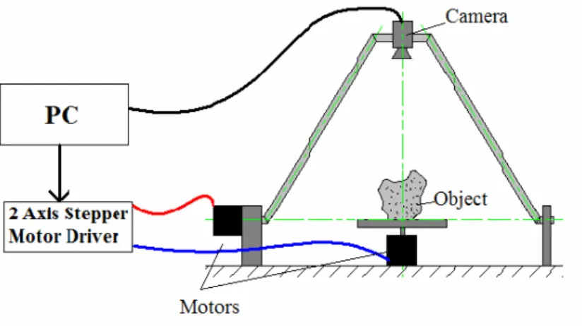
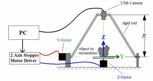
Instead of moving the camera in 2 degrees of freedom (DOF) to get spherical spiral scan (SSS); 1 DOF camera move and 1 DOF object move is used to get the same effect. SSS is detailed in Chapter 4. General sytem setup illustration can be seen in Figure 1.1.
Figure 1.1. General system setup illustration.
The main focus of the thesis is; recovering and tracking some 2D feature points on the images of the objects while object and camera are rotated in controlled angles
After completing SSS, 3D positions of feature points are determined. Then surface fitting algorithm is applied to the 3D feature points.
This thesis is organized as follows:
Chapter 2 gives a brief overview of camera calibration. Chapter 3 gives the background for the use of stereo vision geometry for acquiring depth information. The developed system setup is described in Chapter 4. The 3D point acquiring algorithm is explained in Chapter 5. Fitting surface to point clouds is the subject of Chapter 6. Finally the thesis ends with a conclusion in Chapter 8.
CHAPTER 2
CAMERA CALIBRATION
Camera calibration can be described as the process of determining intrinsic parameters (camera center, focal length, skew factor, radial distortion coefficients) and extrinsic prameters (rotation and translation from world coordinates) of the camera. In Section 2.1 pinhole camera model is described briefly. Section 2.2 and Section 2.3 give brief describtion about intrinsic and extrinsic camera calibration respectively.
2.1. Pinhole Camera Model (Perspective Projection Model)
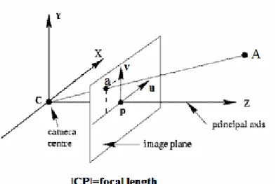
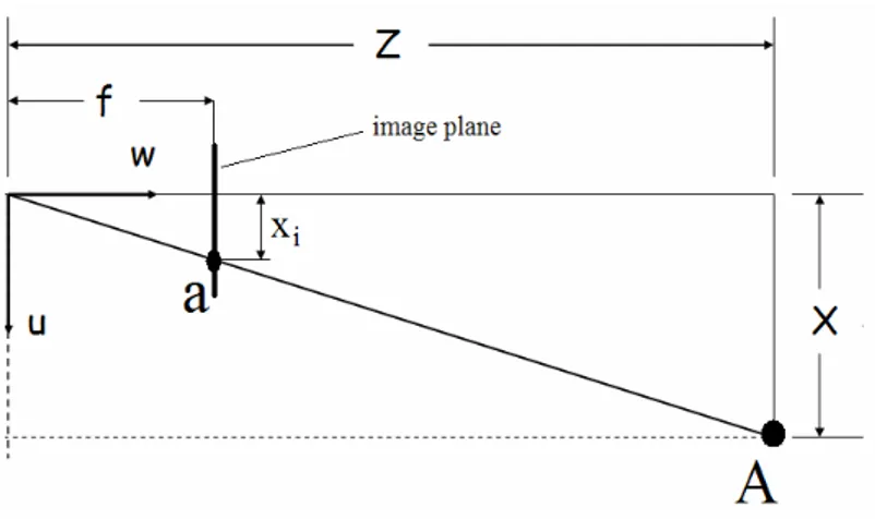
In pinhole camera model, all rays pass from a point called optical center (C) and intersects with the image plane at a distance f (focal length). For simlicity the image plane is considered to be in front of camera center instead of back (real image plane). This is called virtual image plane and an illustration of pinhole camera model with virtual image plane can be seen in Figure 2.1. In pinhole camera model, images are formed on image plane via perspective projection.
Figure 2.1. Pinhole camera model. (Source: WEB_1)
Figure 2.2. Side view of pinhole camera model. (Source: (WEB_1)
Considering any 3D point A(x,y,z) in front of the camera, its image coordinates a(
x
i,y
i) will be;z
x
f
x
i=
z
y
f
y
i=
These equations can be easly obtained by using geometrical similarities of triangles (see Figure 2.2). This transformation can be represented by the following matrix equation:
=
1
0
1
0
0
0
0
0
0
0
0
z
y
x
f
f
w
v
u
(2.1) Wherew
u
x
i=
w
v
y
i=
2.2. Intrinsic Camera Calibration
Real cameras are not exactly same as the simplified camera models (e.g Pinhole camera model, see Figure 2.1) they have some faults due to physical limitations and the production process. These faults are briefly given below.
Image center. Usually principal axis does not passes through center of image
plane. In the ideal case image center is at (width/2)u, (height/2)v . But in reality, this is
not the case. We should take into account the offset from the ideal center, the projection matrix becomes;
=
1
0
1
0
0
0
0
0
0
0 0z
y
x
v
f
u
f
w
v
u
(2.2)Where
u
0 andv
0 are optical center in u and v direction respectively.
Figure 2.3. Scaling factor.
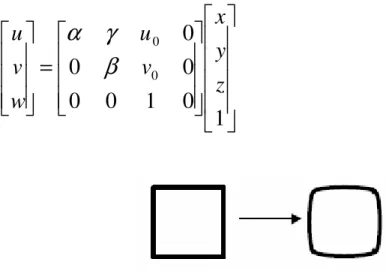
Different scaling factors for u and v direction (e.g. as in Figure 2.3) is necessary especially when the CCD sensors have rectangular geometry. The projection matrix can be modified as following to create this effect:
=
1
0
1
0
0
0
0
0
0
0 0z
y
x
v
u
w
v
u
β
α
(2.3)where
α
=
k
xf
andβ
=
k
yf
. Herek
x andk
y are different scaling coefficients in uand v directions respectively.
Figure 2.4. Skew factor.
Skew factor. This is the fault that the angle between u and v direction is not 90º
(see Figure 2.4). A small modification in the projection matrix can correct this effect.
=
1
0
1
0
0
0
0
0
0 0z
y
x
v
u
w
v
u
β
γ
α
(2.4)Figure 2.5. Radial (Barrel) distortion.
Radial distrortion is caused by imperfections in lens design. Radial distortion
makes straight lines seem curved in image plane (see Figure 2.5 and Figure 2.6a). Radial distortion is a non linear deformation which can not be handled by modifying the projection matrix. It is usually handled by approximating the deformation by a polynomial;
+
+
+
=
′
r
ar
2br
3r
where ( r , r′) are the (ideal, distorted) distance of an image point to center and a, b are the parameters of the transform. Usually, the higher degrees of the polynomial are ignored.
If we re-arrange the 3x4 projection matrix given in equation 2.4 we get;
[
3 3]
0 0 0 00
|
0
1
0
0
0
0
1
0
0
0
0
1
1
0
0
0
0
1
0
0
0
0
0
I
K
v
u
v
u
=
=
β
γ
α
β
γ
α
(2.5)In equation 2.5 K is the camera intrinsic matrix. For metric reconstruction; camera center, focal length, skew factor and radial distrortion coefficients have to be known and have to be corrected before processing the images. Camera intrinsic parameters are usually given in camera intrinsic matrix as follows:
=
1
0
0
0
0 0v
u
K
β
γ
α
(2.6)In equation 2.6 u0 and v0are cooridinates of principal point in u and v directions
respectively,
α
and β are pixel unit focal lengths in u and v directions respectively, γ is skewness factor. Radial distortion parameters a and b are also considered as intrinsic camera parameters.In this paper we do not focus on solving the calibration parameters. For further information about camera calibration, readers may refer to “(Zhang 1999)” and “(Zhang 2000)”.
Matlab Camera Calibration Toolbox (based on “(Zhang 1999)”) is used here to compute the intrinsic parameters of the camera. Then camera intrinsic matrix is manually passed to OpenCV for further steps.
Figure 2.6. Images of same scene taken with a short focal length camera with severe barrel distortion (a) and long focal length camera with low distortion (b). (Source: Hartley et al. 2002)
2.2.1. Intrinsic Camera Calibration Using Matlab Camera Calibration
Toolbox
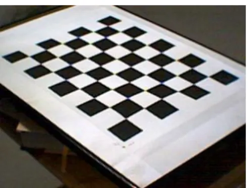
Matlab Camera Calibration Toolbox is based on “(Zhang 1999)”. The toolbox uses at least two views of a planar pattern taken from different orientations. The pattern metrics have to be known and entered to the toolbox before calibration process. Such a pattern consists of 7x9 squares each of which has the size of 30x30 milimeters. The calibration pattern used in this thesis can be seen in Figure 2.7.
The user has to click on corresponding corner points at different views. These points are used for calibration. The more views are used in process, more sensitive calibration parameters are extracted. In this study 5 images of calibration pattern are used. One of these images can be seen in Figure 2.7.
In equation 2.7 Matlab intrinsic parameter result for our camera (an inexpensive USB camera) is shown. γ =0 in the matrix that means angle between u and v is 90º
= 1 0 0 115.21561 447.42302 0 140.14484 0 445.89271 K (2.7)
Besides, radial distortion coefficients calculated by the toolbox are:
Kc = [ -0.30414 0.42971 -0.00017 -0.00684 ] (2.8)
The toolbox can also undistort the images using camera intrinsic parameters. An example of an image before and after undistortion process is shown in Figure 2.8. Radial distortion effect can be seen in Figure 2.8 (a). The bended table edge can be easily seen in the image caused by radial distortion. The same image after undistorting with straight table edge can be seen in Figure 2.8 (b).
(a) (b)
Figure 2.8. (a) An image before undistort process (b) after undistort process. (Source: Hartley et al. 2002)
2.3. Extrinsic Camera Calibration
matrix. These parameters are combined in a single transform matrix. Then any 3D point can be converted from world coordinates to camera coordinates using transform matrix. Once we get the coordinates of 3D points in camera coordinates, then we can easily find 2D image coordinates of those points using projection matrix described in Section 2.1 and Section 2.2.
Figure 2.9. Position and orientation of pinhole camera in world coordinates. (Source: Hartley et al. 2002)
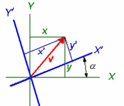
For a 2D vector v, reference system rotation about Z axis, equations can be given as below (see Figure 2.10):
Figure 2.10 A 2D Vector v in two different reference sytems ( XY and YX ′′ ).
) sin( . ) cos( . α y α x x′= + ) sin( . ) cos( . α x α y y′= −
In matrix form; − = ′ ′ y x y x ) cos( ) sin( ) sin( ) cos(
α
α
α
α
If we expand it to 3D; rotation about Z axis can be given as below:
) sin( . ) cos( .
α
yα
x x′= + ) sin( . ) cos( .α
xα
y y′= − z z′= In matrix form; − = ′ ′ ′ z y x z y x 1 0 0 0 ) cos( ) sin( 0 ) sin( ) cos(α
α
α
α
Then rotation matrix around z axis is:
− = 1 0 0 0 ) cos( ) sin( 0 ) sin( ) cos( ) (
α
α
α
α
α
z R (2.9)When we extend equation 2.9 to rotation about y and x axises the full rotation matrix (R) becomes: (2.10) Rz Ry Rx
−
−
−
=
)
cos(
)
sin(
0
)
sin(
)
cos(
0
0
0
1
cos
0
sin
0
1
0
sin
0
cos
1
0
0
0
)
cos(
)
sin(
0
)
sin(
)
cos(
φ
φ
φ
φ
β
β
β
β
α
α
α
α
R
Translation matrix is given as follows: = 1 0 0 0 1 0 0 0 1 0 0 0 1 Z Y X T (2.11)
where X, Y and Z are new world coordinates of the camera.
In this study we used stepper motors to rotate the camera and objects so we know the rotation angles around x-y-z (
φ
,β
,α
) in each step. We also used a fixed radius rod to place the camera. So we can easily calculate 3D position of the camera in world coordinates using rotation angles and fixed radius (R). R is the distance from projection center of the camera to world reference point (0,0,0). Details about experimental setup and the calculation of rotation and orientation are given in Chapter 4.CHAPTER 3
3D RECONSTRUCTION FROM MULTIPLE VIEWS
3.1. Single View Geometry
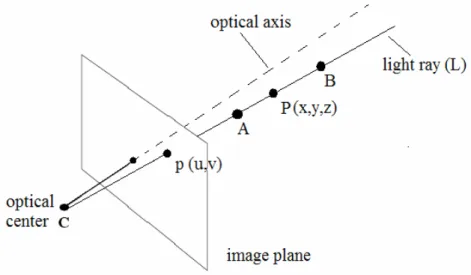
3D reconstruction is the problem of acquiring 3D points of scenes or objects from their 2D image views. Looking at a single 2D image, the depth (3rd dimention) is not directly accesible even for a human. This can be explained easily; supposing that there is a light ray (L) from real point P to image plane that passes through optical center (perspective projection). p is the perspective projection of point P on to image plane. The point p(u,v) on the image plane, which is the projection of a single point P(x,y,z) does not carry any information on where P is located along the ray (L). See Figure 3.1.
Figure 3.1. Missing of depth while projecting.
As can be seen in Figure 3.1, projected coordinates of 3D points A,P and B are (u,v). Although 3D coordinates are different, their image coordinates are same. 3D reconstruction is the inverse process of projection. Given 2D coordinates of a point p, we have to determine which 3D point corresponds to p. It is clear that a single view is
3.2. Two View Geometry (Stereo Vision)
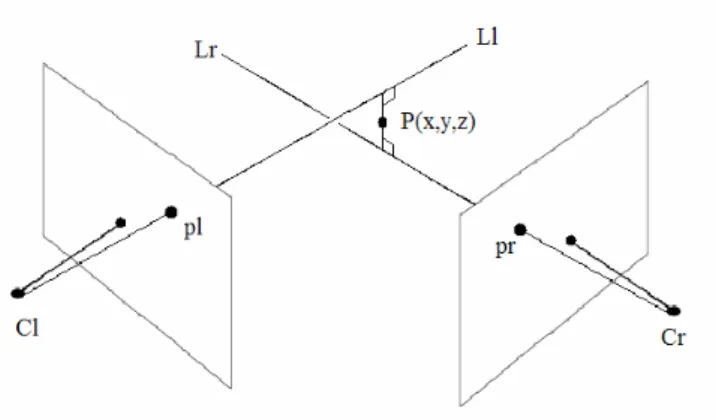
Assume that there are two fully calibrated cameras (i.e. camera centers, focal lengths, pixel ratios, skewness, radial distrortion coeffitions, 3d positions and orientations in world coordiantes are known) as illustrated in Figure 3.2. Both cameras are observing the same scene/object. Suppose that there is a point (P) in the scene visible in both left and right cameras. Let (pl) be the projection of (P) onto left camera’s image plane and (pr) be the projection of (P) onto right camera’s image plane. Since image coordinates of (pl), (pr) and camera parameters are known, (P) can be reconstructed as intersection of two light rays (Ll) and (Lr).
Figure 3.2. Stereo vision.
In practice, two rays will not intersect due to calibration, feature localization and feature tracking errors (see Figure 3.3). However, the 3D position of P(x,y,z) can still be estimated. The approach used in this study is to construct a line segment perpendicular to the two rays where two rays are closest to each other. And then the mid point of the line segment is used as the reconstructed point. “(Forsyth et al.2003)”. When this line segment is longer than a predetermined thresholding value; the reconstructed point is determined as wrong reconstructed point. And the wrong reconstructed points are not recorded as reconstructed points.
In practice, the biggest problem of stereo vision is correspondence problem. Correspondence problem is the problem of finding which point on left image matches which point on right image or vice versa. There are different solutions for correspondence problem in literature. In this thesis, a different technique is used to deal
with correspondence problem. That is why we do not focus on solving the corrsepondence problem in this thesis. The readers who are interested in solving the correspondence problem directed to “(Forsyth et al.2003)” and “(Hartley et al 2002)”.
In this thesis, a moving camera and moving object are used to form stereo vision. An optical flow based tracking algorithm “(Lucas et al. 1981)” is used to avoid correspondence problem. The tracking algorithm enables us to track the feature points in each view, so we know corresponding 2D image coordinates of feature points. Since stepper motor driven objects’/scenes’ feature points displacement are small enough in images, tracking algorithm easily tracks feature points without losing them. The OpenCV implementation of Lucas&Kanade Pyramidial Tracking Algorithm is used in this study.
Figure 3.3. Crossing lines in stereo vision.
The realistic model illustrated in Figure 3.3 is used in this study for 3D reconstruction
Given camera parameters and feature correspondence in two views, the goal is to reconstruct 3D positions of feature points. One should keep in mind that intrinsic camera parameters are pre-calculated for later use, and extrinsic parameters are calculated once in a few steps of stepper motors. Extrinsic parameters (translation and orientation) of camera are easily calculated using rotation angles of stepper motors. Calculation of camera’s 3D position and orientation will be explained in next chapter. Here we will assume that intrinsic and extrinsic parameters are known, and we will just focus on how to reconstruct 3D point using 3D geometry.
CHAPTER 4
EXPERIMENTAL SETUP:
SPHERICAL SPIRAL SCAN MECHANISM
Classical turn-table based 3D reconstruction approaches in stereo vision usually uses single axis rotation tables “(Mülayim et al. 2003)” , “(Williams 2003)”, “(Fremont, V., and Chellali R. 2004)”. Single axis rotation tables gives limited view of the object. In this study we developed a 2 degree of freedom (DOF) system to get more views of the object. Our 2DOF setup moves the camera in a hemispherical spiral trajectory. Camera’s optical axis is oriented to observe the object(s) while it is moving in spherical trajectory.
Figure 4.1. Illustration of experimetal setup used in this thesis.
The spherical and cartesian coordinates can be related by:
) cos( ) sin( ) sin( ) cos( ) sin(
β
α
β
α
β
= = = z y x (4.1)If we extend the unit sphere to R radius sphere; equations in 4.1 become: ) cos( ) sin( ) sin( ) cos( ) sin(
β
α
β
α
β
R z R y R x = = = (4.2)where R is distance from camera optical center to world coordinate system origin in this study (see Figure 4.2).
(a)
(b)
Figure 4.3. A 2-turn spherical spiral, world and camera coordinate systems used in the thesis. (a) side view and (b) top view.
Experimental setup used in this thesis consists of two stepper motors, two stepper motor drivers controlled by PC parallel port and a USB camera. One of the stepper motors is placed vertically and the other is placed horizontally so that their axises are perpendicular to each other. The intersection point of these axises ( see Figure
1.1 and Figure 4.3) is accepted as the origin of the world coordinate system (WCS) (X-Y-Z). Z-axis is chosen to be along vertical motor axis and Y-axis is chosen to be along horizontal motor axis. From now on we will call vertical motor as z-motor because it rotates the object around Z axis. And we will call horizontal motor as y-motor because it rotates the camera around Y axis. Camera coordiante system (CCS) (i-j-k) is illustrated in Figure 4.3. Camera optical axis is always aligned with the line that passes through the origin of CCS and the origin of WCS.
Figure 4.4. shows change of z and y motor rotation angle (
α
,β
) in time t while SSS is in process.Figure 4.4. Rotation angle-time graph in spherical spiral scan process.
4.1. Stepper Motors
Stepper motors are electromechanical devices that converts electrical pulses to shaft (rotor) rotations. A stepper motor consists of a static body (stator) and rotating shaft (rotor). The rotors have permanent magnets attached to them. Around the stators there are series of coils that create magnetic field. When motor is energyzed, permanent magents and coils interacts with each other. If coils are energized in a sequence, the rotor rotates forward or backwards. Figure 4.6 shows a typical stepper motor.
Figure 4.6. Stepper motor.
Stepper motor rotors rotate in certain angles that is dependent on number of phases and number of rotor teeth they have. And rotation angle per step is calculated with the formula given below,
r s m.N
360
=
θ
(4.3)where m is the number of phases and Nris the number of rotor poles (See Figure 4.6). Both z-motor and y-motor used in this study has 4 phases and 50 rotor teeth so they have
8 . 1 50 . 4 360 = = s
θ
(4.4)step degree. In our experiments each step corresponds to 81. .Each motor needs 200 steps for 360 rotation. To complete 2-turn SSS process in “t” time (See Figure 4.3),
z-motor has to rotate 720 (or 400 steps) and in the same time y-z-motor has to rotate 90 (or 50 steps). That means y-motor has to rotate one step ( 81. ) in eachs 8 steps (14.4 ) of z-motor. When we use this information in the coordinate transformations (Eq.4.2), the spherical spiral trajectory can be computed as shown in Figure 4.7.
(a) (b)
(c)
Figure 4.7. Discrete spherical spiral formed by stepper motors.
In Figure 4.7 there are 400 points that cover 400* 81. = 720 (2-turn spherical spiral). That means
α
starts from 0 and increases to 720 . Andβ
starts from 90 and decreases 81. in each 14.4 step ofα
.Stepper motors can also be driven in half step mode with a 90 step angle. But . 8
.
Figure 4.8 shows an image sequence of a test object observed by the camera over the spherical spiral trajectory.
CHAPTER 5
3D RECONSTRUCTION ALGORITHM
A flow chart of the proposed 3D reconstruction algorithm can be seen in Figure 1.3. The algorithm is built on Intel’s OpenCV library to be able to use many pre-implemented codes, such as image capturing function cvCaptureFromCAM(), undistorting function cvUnDistortOnce(), feature point detection function
cvGoodFeaturesToTrack(), optical flow based function for feature point tracking cvCalcOpticalFlowPyrLK() etc.
In this study we captured 320x240 pixel images with 24 bit color depth in RGB with an inexpensive USB camera. Since color is not completely necessary in this application, we converted the images to 8 bit depth gray-scale images. After an initial camera calibration step, the following procedure is implemented.
Reconstruction process starts at the side of the hemispherical spiral (
α
=0 and 90=
β
) and it ends in end point of the spiral (α
=720 andβ
=0 ) (See Figure 4.2 and Figure 4.7). Considering Figure 4.7 it can be seen that the reconstuction algorithm consists of 400 step. In each step, a new image is captured, feature points are detected on the image or tracked (if already detected).Once in every 10 steps (18°) 3D reconstruction is done using the algorithm
explained in Section 3.2 and feature points are cleared. New feature points are re-detected on the image, z-motor and y-motor (so the camera) are driven to next positions via parallel port of the computer. The biggest problem of reconstruction once in every 10 steps (18°) is that; sensitivity of reconstruction is decreasing when camera optical
axis come near parallel to Z axis of WCS. It is because when the angle between two camera’s optical axis is decrease; the position of reconstructued point change in great value corresponding to small angle changes. To alleviate this problem we used an uniform angle in 3D to make sure that angle between two optical axises are not less than some value (i.e. 18°). On the other hand once in 10 step reconstruction has uniform
1. α =0 2.
β
=903. get new image from the camera (I1)
4. undistort the (I1) image (using intrinsic parameters of camera)
5. detect feature points on the image
6. store image coordinates of feature points on memory (L)
7. for step=1 to 400 ; step=step+1
8. get new image from the camera (I2) 9. undistort the I2 image
10. track feature points on I1 and I2 using optical flow
11. store new image coordinates of feature points on memory (R)
12. if (step mod 10 = 0)
13. 3d reconstruction using stored image coordiantes (L and R) (See Section 3.2)
14. reset feature points (clear all feature points)
15. detect feature points on the image
(new feature points are detected on the same image) 16. store feature point image coordinates on memory (L)
17. end if
18. rotate z-motor one step forward 19.
α
=step*1.8 (orα
=α
+1.8 )20. if (step mod 8 =0 )
21. rotate y-motor one step forward 22.
β
=β
−1.823. end if 24. end for
Key decisions such as 2-turns of spherical spiral and one reconstruction in each of 10 steps are made based on results from initial experiments. Underlined parts of the algorithm will be explained in the rest of this chapter.
Before 3D reconstruction algorithm runs; the object has to be placed to the WCS origin and motors have to be placed to their startup position (
α
=00 andβ
=900, seeFigure 4.3). Descriptions of underlined steps of the algorithm are given in followig sections.
The algorithm works as follows:
First, the camera startup position is initialized (line 1 and line 2. Then a new image is captured from the USB camera and undistorted (line 3 and line 4). Feature points of the image are detected in line 5 (see Section 5.1) and stored in memory (line 6). After these initialization steps, SSS processes start in line 7:
A counter counts from 1 to 400 while the object rotates 720° (400 steps of 1.8°
turns)(lines 18, 19). At each 8th step; camera rotates one step (1.8°) (lines 20,21,22,23).
This relative movement makes the camera move in a spherical trajectory (see Figure 4.4 and Figure 4.7). In each of 400 steps feature points are tracked and stored in the memory (lines 8,9,10,11). At each 10th step of the counter; 3D reconstruction is done (line 13). After reconstruction is done, scanning process is restarted with cleared feature point coordinates (lines 14,15,16). While features are being reinitialized (lines 15 and 16) camera position is stationary.
5.1. Feature Point Detection
A feature point is a point in an image that has a well-defined position and can be robustly detected “(WEB_3 2005)”. As in many computer vision applications, corners are chosen to be used as feature points. In this study cvGoodFeaturesToTrack() function of OpenCV library is used. This algorithm determines strong corners on images “(WEB_2 2004)” . A corner on images is searched in a small region of interest using eigenvalues of the matrix shown below. A point on an image is identified as a corner when eigenvalues corresponding to that point have high values.
=
y y x y x xD
D
D
D
D
D
C
2 2 (5.1)where D and x D are the first derivatives in x and y directions respectively “(WEB_2 y
2004)”. Above matrix is calculated for all pixel points on the image with a small region of interest. Eigenvalues are found by solving a linear system corresponding to nxn matrix A.
AX
=λ
X
(5.2)The scalar
λ
is called eigenvalue ofA
corresponding to eigenvector0
≠
∈
R
nX
“(WEB_4 2006)”. Equation 5.2 can also be written as:0
)
(
A
−
λ
I
X
=
(5.3)where
I
is the identity matrix. Equation 5.3 leads to0
)
det(
A
− I
λ
=
(5.4)When we solve equation 5.4 for the 2x2 matrix given in equation 5.1 then eigenvalues can be written in closed form as: “(WEB_2 2004)”.
− − + ± + = ( ) 4( ( ) ) 2 1 2 2 2 2 2 2 2 2 2 , 1 D x D y D x D y D x D y DxDy λ (5.5)
If
λ
1≈
0
andλ
2≈
0
then there is no feature in this pixel, ifλ
1≈
0
andλ
2 isequal to some large positive value then an edge is found in that pixel, if both
λ
1 andλ
2are large values, then a corner is found “(WEB_5 2005)” . These corners can be refined using some threshold value (t). If
λ
1>λ
2>t where t is some threshold, pixels that havetheir eigenvalues less than t are eliminated and not considered as corner points.
The feature detection algorithm “cvGoodFeaturesToTrack()” that is built in OpenCV works as follow: “The function first calculates the minimal eigenvalue for every pixel of the source image and then performs non-maxima suppression (only local maxima in 3x3 neighborhood remain). The next step is rejecting the corners with the
function ensures that all the corners found are distanced enough from one another by getting two strongest features and checking that the distance between the points is satisfactory. If not, the point is rejected” “(WEB_2 2004)”.
The function takes source image, 2 image memory for eigenvalues calculation process, a multiplier value (quality level) which specifies minimal accepted quality of image corners, a limit value which specifies minimum possible Euclidean distance between returned corners as input parameters. It returns number of detected corners and image coordinates of detected corners. In experiments 0.01 multiplier used for quality level of corners and 10 pixel distance is used for possible distance between each corners detected.
In this study we worked on two objects for reconstruction. First one is a well textured box like object made of paper. This object has no concavities on its surfaces so it is relatively easy object to reconstruct. Second object we used is piece of egg carton, relatively complex due to its concavities on surfaces and being not well textured. We put additional paints on its surface to simplify feature detection and tracking. Images of original objects are shown in Figure 5.2.
(a) (b)
Figure 5.2. Test objects used in this thesis for 3D reconstruction. (a) a box (b) a piece of egg carton.
Figure 5.3 shows images of test objects after feature point detection algorithm. Feature points are represented as bold circles.
(a) (b)
Figure 5.3. Feature point detected images of test objects (a) box image with 118 detected feature points (b) egg carton with 97 detected feature points.
5.2. Tracking of Feature Points
Tracking of feature points while camera is moving on its spherical spiral trajectory alleviates the correspondence problem. Since losing tracking of feature points will cause reconstruction of the points in incorrect positions, feature tracking is one of the most fundamental steps in this study. In order to track a pixel in an image its velocity vectors have to be calculated. This representation is called velocity field or optical flow field of the image.
Optical flow methods try to calculate the motion between two image frames that are taken at times t and t+ t∆ . Optical flow can be defined as an apparent motion of
images brightness. Let I(x,y,t) be the image brightness at time t of an image sequence. Main assumptions on calculating optical flow is that: Brightness smoothly depends on a particular image coordinates in greater part of the image. Brightness of every point of a moving or static object does not change in time “(WEB_2 2004)”.
Optical flow field calculated from image sequence of rotating sphere is given below.
Image #1 Image #2 Optical Flow Field
Figure 5.4. A rotating sphere from left to right and corresponding optical flow field (Source: WEB_6 2006)
If some point in an image is moving, t∆ time later the point displacement is
( x∆ , y∆ ). When Taylor series for brightness I(x,y,t) is written:
c dt t I dy y I dx x I t y x I t t y y x x I + ∂ ∂ + ∂ ∂ + ∂ ∂ + = ∆ + ∆ + ∆ + , , ) ( , , ) ( (5.6)
where c represents the higher order terms which are small enough to be ignored. When above assumptions are applied to equation 5.6, we have,
) , , ( ) , , (x x y y t t I x y t I +∆ +∆ +∆ = (5.7) and 0 = ∂ ∂ + ∂ ∂ + ∂ ∂ dt t I dy y I dx x I (5.8)
Dividing equation 5.8 by dt and re-arranging equation 5.8 such that
u dt dx = (5.9) v dt dy = (5.10)
where u and v are speeds of point moving in x and y directions respectively, gives the equation called optical flow constraint equation:
v y I u x I t I ∂ ∂ + ∂ ∂ = ∂ ∂ − . (5.11) In equation 5.11 t I ∂ ∂
term is about how fast the intensity chages at a given pixel
in time. x I ∂ ∂ and y I ∂ ∂
are about how rapidly intensity chages on going across the picture. Different solutions to equation 5.11 are given in “(Lucas and Kanade, 1981)” and “(Horn and Schunck,1981)”. We have used OpenCV implemetation of optical flow calculation which uses the Pyramidial Lucas&Kanade Technique. Readers who are interested in details about Lucas&Kanade technique should refer to “(Lucas et al. 1981)”.
Figure 5.5 shows a sequence of images while 112 feature points are being tracked. It can be easily seen that the box rotates in counterclockwise direction (also can be imagined as camera rotation around the objectin clockwise direction). Figure 5.6 shows a sequences of egg carton images with 101 feature points being tracked. Image coordinates of all feature points are recorded in tracking process. (Coordinates (x,y) of an arbitrary feature point are also given in Figure 5.5.)
(148,170) (a) Image #1 (159,167) (b) Image #2 (171,166) (c) Image #3
(a) Image #1
(b) Image #2
5.3. 3D Reconstruction of Tracked Feature Points
Given camera parameters and feature point correspondences obtained by tracking in two views, the goal will be to reconstruct the 3D coordinates of the feature point. Lets write camera’s 3D positions in matrix format assuming that cameras are reduced to one point (optical center). Coordinates of the left camera,
= l l l l z y x C (5.12)
coordinates of the right camera:
= r r r r z y x C (5.13)
Since we know the spherical coordinates of the camera defined by
α
,β
and R , cartesian camera coordinates (x,y,z) can be calculated easily by using equation 4.2. Whereα
andβ
are stepper motor’s rotation angles in current position of camera and R is the radius of the sphere shown in Figure 4.1.Image coordinates of any feature point (p) on left image,
= l l l j i p (5.14)
corresponding coordinate of same feature point on right image is:
= r r r j i p (5.15)
where i and j are image coordinates in u and v directions respectively. First we have to reconstruct two light rays (lines) L and l Lr. A 3D line equation in parametric form can be written as:
V t P
L= 0 + (5.16)
where P is start point of line, t is the parameter whose value is varied to define points 0
on the line and V is a vector defining the direction of the line. When we write the lines
l
L and Lrstarting from camera’s optical centers;
w l l l l
C
t
V
L
=
+
(5.17) and w r r r rC
t
V
L
=
+
(5.18)In equation 5.17 and 5.18; t and l tr are parameters that define points on both
lines. w l
V and w r
V are vectors that define directions of both lines L and l Lr. We should
keep in mind that all variables given above are in WCS.
Since the only apriori information is on the image coordinates of feature points,
w l
V and w r
V can be obtained by applying rotation matrix to CCS vectors Vl and V , r
where Vl and V are unit vectors from optical center to feature points on the image r
Figure 5.7. The vector defining the direction of reconstruction lines.
The 3D positions of the feature point p and the optical center C are: = z y x p p p p or p= pxi + pyj+ pzk (5.19) = z y x C C C C or C=Cxi +Cyj+Czk (5.20)
then reconstruction line direction vector V is:
C p V = − or − − − = z z y y x x C p C p C p V (5.21)
C is the origin of the camera coordinate system so C =0i +0j +0k and all images on image plane has 3rd coordinates equal to camera’s focal length. If we put these together
= f p p V y x (5.22)
where p and x p are feature point coordinates on image in u and v directions y
respectively and f is focal length (in terms of pixels) pre calculated during camera calibration. If pixels are not squares p , x p and f have to be adjusted accordingly. y
The camera used in this study has square pixels. If we write feature point coordinates in vector format using equation 5.14 and 5.15.
= f j i V l l l or Vl =ili + jlj+ fk (5.23) And = f j i V r r r or Vr =iri + jrj + fk (5.24)
Equation 5.23 and 5.24 are direction vectors in camera coordinate system. Before using them in equation 5.17 and 5.18 they have to be converted to world coordinate sytem using transformation matrix. If w
l
V and w r
V are corresponding unit
WCS vectors of Vl and V then r
= w l w l w l w l k j i V (5.25) = w w r w j i V (5.26)
when we rewrite equation 5.17 and 5.18; + = w l w l w l l l l l l k j i t z y x L (5.27) + = w r w r w r r r r r r k j i t z y x L (5.28)
In equation 5.27 and 5.28 we can see that parametric equations of two lines are fully known. Next step is finding the intersection point or more generally finding the 3D point that is closest to the two lines (see Figure 3.3).
Parameters that makes two lines closest to each other are given by
2
b
ac
cd
be
t
c l−
−
=
(5.29) 2b
ac
bd
ae
t
c r−
−
=
(5.30) w l w lV
V
a
=
•
w r w l
V
V
b
=
•
w r w r
V
V
c
=
•
S
V
d
w l•
=
S
V
e
w r•
=
where
S
=
C
l−
C
r and (• ) denotes dot products of vectors. Applying equation 5.29between these two points is retrieved as the 3D reconstructed point of the observed feature point.
Applying reconstruction process to all feature points, a set of 3D points are acquired. These points can be considered as “point clouds” with no structural information. The next step is fitting a mathematical model to the point clouds (so-called “surface fitting”). Figure 5.8 shows reconstructed point clouds of test objects.
(a)
(b)
Incorrect reconstructed points on the top of the box
CHAPTER 6
SURFACE FITTING
The final step of the 3D reconstruction procedure presented in this thesis is fitting a parameterized 3D model to the acquired point clouds. After fitting such a model to point clouds, various high level computer vision process can be applied to the 3D scene, such as texture mapping, 3D object recognition etc. There are many surface fitting techniques in literature “(Siddiqui, M. and Sclaroff, S. 2002a)”, “(Zwicker et al. 2004)”, “(Yvart et al 2005)” . The presented method for surface fitting is quite easy and fast, although it cannot be applied to objects with various topologies.
The technique is based on projecting all reconstructed points on to an initial meshed hemisphere that covers all points, and back projecting the hemisphere’s meshpoints towards the point clouds. Choosing radius of hemisphere (R), equal to radius of spherical spiral (see Chapter 4) is a good idea, since we know that all reconstructed points will be inside the hemisphere. When an (mxn) meshed, R radius hemisphere is initialized all points are projected on to the hemisphere recording their vector magnitudes (Here all reconstructed points and mesh points are represented as vectors where start point of vectors are WCS origin and end points are 3D point coordnates). Then new coordinates of mesh points are calculated with the help of projected vector’s magnitudes. The average of k-nearest vector magnitudes are set to be the magnitudes of mesh points. Finally initial vector magnitude of mesh point is replaced with that average magnitude keeping the direction of the initial vector. Surface fitting algorithm is given below (also see Figure 6.1):
1. create a hemisphere with mesh interval (mxn)
2. project all points on to hemisphere recording the directions and magnitudes.
3. for all mesh points (mxn)
a. find k-nearest projected vectors on hemisphere to the mesh point (m,n)
b. calculate average magnitude of k-nearest vectors on the hemisphere
c. set new magnitude of mesh point as calculated average magnitude
Figure 6.1. A meshed hemisphere with 20x15 Intervals.
In the subject of surface fitting, we also worked on synthetic data points. These point clouds consist of 50400 points. Although the points are created using mathematical equations, the relations between points are assumed not to be known in the surface fitting process. These synthetic data helped us to observe the performance of surface fitting on point clouds. Figure 6.2.a shows point clouds corresponding to a synthetic object, while Figure 6.2.b shows points projected on the hemisphere and Figure 6.2.c shows back-projected (fitted) hemisphere on the point clouds. During surface fitting to synthetic data 10 nearest vectors are used to calculate the new magnitude of mesh point.
(a) (b) (c)
Figure 6.2. A synthetic data set with 50400 points (a), projected data points on to hemisphere (b) and fitted surface on to data points with mesh size (25x20) Figure 6.3 shows fitted surface to test object point clouds.
(a) Isometric view of egg carton point clouds
clouds (2033 points) (b) fitted surface to egg carton point (25x20 size mesh)
(c) Top view of box point clouds
Figure 6.4 shows a smooth surface model of the egg carton. Fit function of The Mathematica software is used to obtain the model. The mathematica code is given below where EggC.txt is the text file that contains reconstructed 3D point coordinates.
xyz = ReadList["c:\EggC.txt", {Real, Real, Real}]; polynomial = Flatten[Table[x^i y^j, {i, 0, 4}, {j, 0, 4}]] f[x_, y_] = Fit[xyz, polynomial, {x, y}]
Plot3D[f[x, y], {x, -70, 70}, { y, -70, 70}, PlotRange -> {-50, 5}, BoxRatios -> {6, 6, 5}, PlotPoints -> 50, ViewPoint -> {1, 2, -2}];
CHAPTER 7
CONCLUSIONS
In this thesis, an electromechanical setup is developed to acquire images of test objects from different view angles. The main difference between the developed setup and the one axis turn table based applications is that the developed setup has two rotational degrees of freedom. We defined a spherical spiral motion around the test object which helped us to get images not only from sides but also from top of the objects. Since stepper motors are used for rotating the camera and objects, some mechanical vibrations occur which cause to lose tracking. These vibrations can be reduced using servomotors instead of the stepper motors. However this solution will increase the cost and the complexity of the system. The inhomogenuity in lighting conditions is another important factor that degrades system perormance.
In the reconstruction process feature tracking algorithm is used to alleviate the point correspondence problem. Reconstruction is done by using stereo vision geometry where one image is assumed to be left image, and second image is assumed to be right image. Feature points are tracked between left and right image. Extrinsic camera parameters of the viewing positions of left and right image are calculated by using stepper motor rotation angles. After reconstructing the points, over spherical spiral trajectory an unorganized point clouds are acquired.
Reconstruction time of an object depends on the trajectory of the camera. Since mechanical vibrations increase with rotation velocity of steppers causing tracking algorithm to lose features, we added some delays between the steps of the algorithm. In this thesis we used a 2-turn spherical spiral trajectory move for the camera where reconstruction time is about 200 seconds. Since mechanical moving time is much greater than the computational time, computational time for reconstruction is ignored.
To reduce incorrect reconstructed points three main process are made. First a thresholding value added to the line segment between crossing lines which was described in Section 3.2. Second process is using uniform angle while reconstructing the points which was described in Chapter 5. And last process was to eliminate the feature points which displacements are small than some thresholding value while
tracking. This process alleviate the incorrect reconstructions of feature points that are collected to the side of objects while the object is rotating.
Surface fitting algorithm presented in this thesis is quite easy and fast compared to iteration based fitting techniques. For a point clouds which contains about 2000 points, to fit 25x20 mesh size surface, complete fitting time is about 1 second on a PC with a Pentium 4, 3GHz CPU, and 512 MB RAM. Although this technique cannot be applied to all kind of objects such as objects with holes, the technique can be used with appropriate objects due to its simplicitiy and speed. Texture mapping which can be considered as a possible next step is not studied in this thesis.
Although the 3D reconstruction and surface fitting results achieved in this thesis are satisfactory, the performance can be significantly improved by hybrid techniques (E.g. combining silhouette based reconstruction techniques and feature tracking based reconstruction techniques).
A more robust electromechanical setup design (minimizing vibrations), refinement in 3D reconstruction, improving surface models and application of texture mapping can be listed as the possible research problems that should be addressed in the future.
BIBLIOGRAPHY
Fremont, V., and Chellali R. 2004 ”Turntable-Based 3D Object Reconstruction”; IEEE Cybernetics and Intelligent Systems Conference, Volume 2, Dec. 2004, pp.1277-1282.
Forsyth, D. A., and Ponce J. 2003 “Computer Vision: A Modern Approach”; Published by Prentice Hall, Upper Saddle River, New Jersey, Jan. 2003.
Hartley, R. and Zisserman A., 2002 “Multiple View Geometry in Computer Vision”; Published by Cambridge University Press, 2002.
Lucas, B. D. and Kanade T. 1981 “An iterative image registration technique with an application to stereo vision”; Proc. 7th Joint Conf. On Artificial Intelligence, Vancouver, BC, 1981, pp.674-679
Mülayim, A. Y., Yılmaz ,U. And Atalay V. 2003. “Silhouette-based 3D Model Reconstruction from Multiple Images”;IEEE Transactions on Systems, Man and Cybernetics, Part B, Volume 33, Issue 4, Aug. 2003, pp.582-591.
Narkbuakaew, W., Pintavirooj C., Withayachumnankul W., Sangworasil M. And Taertulakarn S. 2005 “3D Modeling from Multiple Projections: Parallel-Beam to Helical Cone-Beam Trajectory”, WSCG SHORT papers proceedings, Czech Republic, Science Press, January 31-February 4, 2005
Sainz, M., Bagherzadeh, N., and Susin, A. 2002. “Carving 3D Models From Uncalibrated Views”; Computer Graphics and Imaging 2002, Track-Image Processing, 358-029
Sainz, M., Pajarola, R., Mercade, A., and Susin, A. 2004 “A Simple Approach for Point-Based Object Capturing and Rendering”; IEEE Computer Graphics and Applications, Volume 24, Issue 4, Aug.2004, pp.24-33.
Siddiqui, M. and Sclaroff, S. 2002a “Surface Reconstruction from Multiple Views using Rational B-Splines”; IEEE 3D Data Processing Visualization and Transmission Symposium, 2002, pp.372-378.
Siddiqui, M. and Sclaroff, S. 2002b “Surface Reconstruction from Multiple Views Using Rational B-Splines and Knot Insertion”; Proceedings First International Symposium on 3D Data Processing Visualization and Transmission, 2002, pp.372-378.
Williams, G. 2003 “Textured 3D Model Reconstruction from Calibrated Images”; University of Cambridge Dissertation 2003
WEB_2, 2004. “Intel Open Source Computer Vision Library Manual”, 20/12/2004. http://www.intel.com/research/mrl/research/opencv/
WEB_3, 2005. “Corner Detection”,9/12/2005, http://en.wikipedia.org/wiki/Corner_detection WEB_4, 2006. “Eigenvalue”, 9/01/2006, http://mathworld.wolfram.com/Eigenvalue.html WEB_5, 2005. “Corner Detection”,9/12/2005, http://mathworld.wolfram.com/Corner_Detection
WEB_6, 2006. “Optical Flow Algorithm Evaluation”, 10/02/2006, http://www.cs.otago.ac.nz/research/vision/Research/OpticalFlow/opticalflow Yvart, A., Hahmann, S., Bonneau, G.P. 2005 “Smooth Adaptive Fitting of 3D Models
Using Hieararchical Triangular Splines”; International Conference on Shape Modeling and Applications, SMI'05, 13-22 (2005) MIT Boston, IEEE Computer Society Press, 2005.
Yemez Y. and Schmitt F., 2004 "3D reconstruction of real objects with high resolution shape and texture,"; Image and Vision Computing, Vol. 22, pp. 1137-1153, 2004.
Zhang, Z. 1999 “Flexible Camera Calibration By Viewing a Plane From Unknown Orientations”; Seventh IEEE International Conference on Computer Vision, Volume 1, Sept 1999, pp.666-673.
Zhang, Z. 2000 “A Flexible New Technique for Camera Calibration”; IEEE Transactions on Pattern Analysis and Machine Intelligence, Volume 22, Issue 11, Nov. 2000, pp.1330-1334
Zwicker, M. and Gotsman, C., 2004 “Meshing Point Clouds Using Spherical Parameterization”; Eurographics Symposium on Point-Based Graphics, Zurich, June 2004.
APPENDIX A
COMPUTER SOFTWARE
In this thesis, Microsoft Visual C++ 6.0 and OpenCV libaray is used to develop the required algorithm. Matlab is also used to calculate the camera intrinsic matrix. The developed 3D reconstruction system is consist of two individual parts. First one is reconstruction and second one is fitting. The programs that includes these algoritms will be briefly described below. These computer programs are given in a CD. This CD also contains a README text file that describes the computer programs.
mscthesis.cpp: This is the source code that contains reconstruction algorithm.
The code originally modified from lkdemo.c which is the demo software of Lucas&Kanade tracking algoirthm supplied by OpenCV Library. This source code gets images from USB camera, controls the electromechanical component via parallel port and writes the reconstruction results into text files.
rotate.h :This source code calculates the rotation matrix needed by mschesis.cpp.
line3d.h: This source code calculates the closest points of two 3D lines. The
code also contains some gemetrical calculations such as intersection of line and plane, plane point distance etc.
SurfaceFit.cpp: This source code takes a text file that contains 3D point
coordinates as an input. The text file is created by mscthesis.cpp. Then this algorithm calculates a surface approximation to that points. Mesh point coordinates are stored in a text file as a result of fitting process.