A SOLUTION METHOD FOR INTEGRO-DIFFERENTIAL EQUATIONS
OF CONFORMABLE FRACTIONAL DERIVATIVE
by
Mustafa BAYRAM a*, Veysel Fuat HATIPOGLU b, Sertan ALKAN c, and Sebahat Ebru DAS d
a Department of Computer Engineering, Gelisim University, Istanbul, Turkey b Department of Business Administration, Mugla Sitki Kocman University, Mugla, Turkey
c Department of Computer Engineering, Iskenderun Technical University, Hatay, Turkey d Department of Mathematics, Yildiz Technical University, Istanbul, Turkey
Original scientific paper https://doi.org/10.2298/TSCI170624266B
The aim of this work is to determine an approximate solution of a fractional or-der Volterra-Fredholm integro-differential equation using by the Sinc-collocation method. Conformable derivative is considered for the fractional derivatives. Some numerical examples having exact solutions are approximately solved. The compar-isons of the exact and the approximate solutions of the examples are presented both in tables and graphical forms.
Key words: Sinc-collocation method, conformable fractional derivative,
Volterra-Fredholm integro-differential equation
Introduction
In recent years, numerous problems from physics, mathematics, biology, chemistry, engineering, and other various sciences involving fractional calculus has been studied by many authors. Several numerical methods for solving linear and non-linear fractional integro-differ-ential equations based on Riemann-Liouville and Caputo derivative have been presented. Many numerical methods such as, wavelets [1, 2], Adomian decomposition method [3, 4], homotopy perturbation method [5], homotopy analysis method [6], and variational iteration method [7] have been used to solve fractional integral equations and integro-differential equations.
In this work, we consider the following form of the fractional Volterra-Fredholm in-tegro-differential equation:
( )
( )( )
( )
( ) ( )
( ) ( )
1 1 , d 2 2 , d x b x yα x f x K x t y t t K x t y t t α α α µ = +λ∫
+λ∫
(1)with the boundary conditions:
( ) 0, ( ) 0
y a = y b = (2)
where y α( ) is the conformable fractional derivative for 1< ≤α 2. Here T fα( ) where t >0 , (0,1)
α ∈ be understood as conformable fractional derivative which was defined in [8]. Some properties of the conformable fractional derivative are given in the next section.
Preliminaries
In this section, the fundamental theorems and definitions are introduced. Readers can look for more details in [9-16].
Definition 1. Let α ∈( ,n n+1] and f be an n-differentiable function at t, where t 0 ,>
Then the conformable fractional derivative of f of order α is defined:
( 1) ( ) ( 1) 0 l m ( ) ( )( ) i f t t f t T f t α α α α α ε ε ε − − − → + − = (3) where α is the smallest integer greater than or equal to α.
Remark 1. As a consequence of Definition 1, one can easily show that:
( ) ( )( )f t ( )t T t α α f α α − = (4)
where α ∈( ,n n+1] and f is (n +1) differentiable at t >0.
Theorem 1. Let α ∈( ,n n+1] and f, g be α-differentiable at a point t >0. Then: (1) T af bgα( + )=aTα( )f +bTα( )g , for all a b∈, ,
(2) T t( )p ptpα
α = − , for all p ∈,
(3) Tα( )λ =0, for all constant functions f t( )=λ,
(4) Tα( )fg = fTα( )g +gT fα( ), and
(5) T ( / ) [f g gT ( )f fT ( ]g) /g2
α = α + α
Definition 2. The function:
sin( ) , 0 sinc( ) 1, 0 x x x x x π ≠ = π = (5) is called the sinc (sinc cardinal) function.
Definition 3. The translated sinc function with space points are defined:
( , )( ) si sin , 1, nc x kh h x kh S k h x x k h h x kh h x kh π − ≠ − π − = = = (6) where h >0 and k =0, 1, 2, ± ± …
For establishing the approximation on ( , )a b , the conformal map is defined:
( )
z In z ab z
φ = − −
(7)
Here, the basis functions are attained using the composite translated sinc functions given:
( ) ( , )( ) ( ) ( ) sinc k z kh S S k h z z h z = οφ = φ − (8) 1( ) 1 w w a be z e w φ− + = = + (9)
is the inverse map of w=φ( )z . The sinc grid points zk∈( , )a b in DE are real numbers, so that
they can denoted by xk. The notation o denotes the Hadamard matrix multiplication. For the
evenly spaced points
{ }
kh k∞=−∞, the image corresponding to these points is defined: 1( ) , 0, 1, 2, 1 kh k kh a be x k e kh φ− + = = = ± ± … + (10)
The sinc-collocation method
Consider the approximate solution of eq. (1) is given:
( ) N ( ) , 1 n k k k M y x c S x n M N =− =
∑
= + + (11)Here, S xk( ) is the composite function of S k h( , ) and φ( )x for some fixed step size h. The
unknown coefficients ck in eq. (11) are obtained with the help of the sinc-collocation method (SCM).
Theorem 2. The conformable fractional derivative of y xn( ) is:
( ) 2
[
]
2 2 2 d d ( ) ( ) , 1 2 d ) d ( ) ( ) N ( n k k k k M x x yα c x α φ x S φ x S x α φ φ − =− ′′ ′ =∑
+ < ≤ (12)Proof. The conformable fractional derivative of y xn( ) can also be written from eq. (11):
( )( ) N ( )( ) n k k k M yα x c Sα x =− =
∑
(13)with the help of eqs. (3) and (4), we have:
( )( ) 2 ''( )
k x k x
Sα =x S−α (14)
When we write eq. (14) in eq. (13), we find that:
( ) 2
[
]
2 2 2 d ( ) ( ) ( ) ( ) d ( d ) d N n k k k k M yα x c x α φ x S x φ x S x φ φ − =− ′′ ′ + =∑
With the aid of Theorem 2.13 in [17], the below two lemmas are presented.
Lemma 1. The following relation provides:
( )1 1 1 ( ) ( , ) , ) ) ( d ( j x N j k jk k k M k a K x t K x t y t t h y t δ φ − =− ′ ≈
∑
∫
(15) where ( )1 0 sin d , 1 2 j k jk tt t jk jk σ = − π δ − = +σ π∫
(16)and yk is the approximate value of y t( )k .
Lemma 2. The following relation provides
2 2( , ) ( )d ((,)) b N k k k M k a K x t K x y t t h y t t φ =− ′ ≈
∑
∫
(17)Replacing each term of eq. (1) with the approach defined in eqs. (11)-(17) and the producing with {(1/ ) }φ′ 2 , we determine:
( ) 2 2 1 1 2 3 4 1 ( ) ( ) ( ) d ( , , ( ) 1 d ) ( ) ( ) ( ) ( ) i N k k k i i k jk k M i k k K x t K x t c g S g g f x t t x x xδ x φ φ φ φ − =− = + + = ′ ′ ′
∑
∑
(18) where ' 2 2 2 1( ) 1( ) , ,2( ) 3( ) 1 1( ) , 4( ) 2 1( ) g x g x g h g h x x x x x x α λ λ φ φ φ − = − = = − = − ′ ′ ′ (19)We know from [18] that:
( )0 ( )0, ( )1 ( )1, ( )2 ( )2
jk kj jk kj jk kj
δ =δ δ = −δ δ =δ (20)
Theorem 3. Let us consider the boundary value problem eqs. (1) and (2). Then the
discrete sinc-collocation system for determining the unknown coefficients N
k M
{ }ck =− of the
ap-proximate solution is given:
( ) ( ) ( ) 1 2 2 1 1 1 2 3 2 2 4 ( ) ( ) ( ) ( ) ( ) ( ) ( ) ( , ( ) 1 , ( ) ) j j j k jk jk j jk N k k j k M j k j j k g x g x K x t g x h h t c f x K x t x g x t δ δ δ φ φ φ − =− + + + = ′ + ′ ′
∑
(21) for j= −M, ,… N.Some notations are defined to rewrite eq. (21) in the matrix form. Let D(y) be a diag-onal matrix whose diagdiag-onal elements are y x( −M), (y x− +M 1), , ( )… y xN and non-diagonal
ele-ments are zero:
1 2 1 2 2 2 , , , ( ( ) ) ( ) ( ) ( ) ( ) j k j k j k j k K x t K x t E E x t x t φ φ φ φ = = ′ ′ ′ ′ (22) denote a matrix and also let I( )i denote the matrices:
( )i ( )i , 1, 0,1, 2 jk I =δ i= − (23) where ( )1 ( )0 ( )1 1 2 , , , , , ,
D G E E I − I I , and I( )2 are n n× matrices. By using the previous notations in
eq. (21), we can represent it:
Ac B= (24) where ( ) ( ) 2 1 3 1 4 2 1 1 ( ) i ( ) ( ) i i i A D g I D g E I D g E h ο − = =
∑
− − (25)( )
2 f B D I φ = ′ (26) 1 ( , , , )T M M N c= c− c− + …c (27)The notation ο in A denotes the Hadamard matrix multiplication. Finally, we can reach the approximate solution of eq. (21) after finding the unknown coefficients ck in the system. Numerical examples
In this section, SCM is applied to two different problems using Mathematica10. In each example, we consider h= π/N1/2 and N M= .
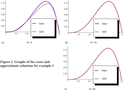
Example 1. Let us take the following boundary value problem:
( ) 1 2 ( ) ( ) x ( , ) ( )d b ( , ) ( )d , (0) 0, (1) 0 a a x x yα = f x + K t y t t+ K xt y t t y = y =
∫
∫
(28) where 1( , ) 2 7 , sin( ), , ) cos( ) 4 K x t x t K (x t x t α= = − = − and(
)
( )
(
)
( )
5 9 2 3 4 4 4 ( ) 24 6 6 12 1217cos 1 30cos 18sin 1 18sin
f x x x x x x x
x x x x
= + + − − − + −
− − − + − +
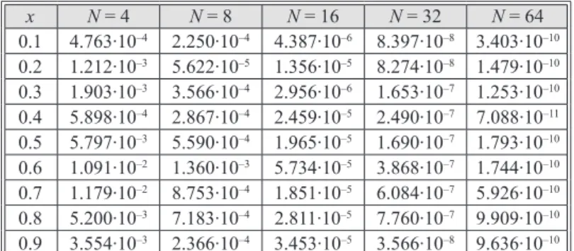
This problem has an exact solution in the form of (x)=x3(1−x). The comparisons of
the exact and the approximate solutions of the example are shown graphically for different N values in fig. 1. In addition, the approximate solution obtained with the aid of SCM of this problem is shown in tab. 1.
(a) N = 4 (b) N = 16 (c) N = 64 Exact SCM Exact SCM Exact SCM (a) N = 4 (b) N = 16 (c) N = 64 Exact SCM Exact SCM Exact SCM
Figure 1. Graphs of the exact and approximate solutions for example 1
Example 2. Let us consider the fractional integro-differential equation:
( ) 1 2 ( ) 2 ( , ) ( )d ( , ) ( )d , (0) 0, (1 0 ) ) ( x b a a yα x = f x − K x t y t t− K x t y t t y = y =
∫
∫
(29)where 2 1( , 2 3 , , ) 2 K x t) x t K ( ,xt x t α= = − = − and
( )
1 2 3 4 20 6 3 6 x x x f x = + x− − +The exact solution of this problem is ( )x =x x( −1). The numerical solutions deter-mined by SCM of the problem are presented in tab. 2. Furthermore, the comparisons of the exact and approximate solutions are given graphically in fig. 2.
Table 1. Errors between the exact and the approximate solution of Example 1
x N = 4 N = 8 N = 16 N = 32 N = 64 0.1 4.763∙10–4 2.250∙10–4 4.387∙10–6 8.397∙10–8 3.403∙10–10 0.2 1.212∙10–3 5.622∙10–5 1.356∙10–5 8.274∙10–8 1.479∙10–10 0.3 1.903∙10–3 3.566∙10–4 2.956∙10–6 1.653∙10–7 1.253∙10–10 0.4 5.898∙10–4 2.867∙10–4 2.459∙10–5 2.490∙10–7 7.088∙10–11 0.5 5.797∙10–3 5.590∙10–4 1.965∙10–5 1.690∙10–7 1.793∙10–10 0.6 1.091∙10–2 1.360∙10–3 5.734∙10–5 3.868∙10–7 1.744∙10–10 0.7 1.179∙10–2 8.753∙10–4 1.851∙10–5 6.084∙10–7 5.926∙10–10 0.8 5.200∙10–3 7.183∙10–4 2.811∙10–5 7.760∙10–7 9.909∙10–10 0.9 3.554∙10–3 2.366∙10–4 3.453∙10–5 3.566∙10–8 9.636∙10–10 (a) N = 4 (b) N = 16 (c) N = 64 Exact SCM Exact SCM Exact SCM (a) N = 4 (b) N = 16 (c) N = 64 Exact SCM Exact SCM Exact
SCM Figure 2. Graphs of the exact and approximate solutions for
Conclusion
This work focused on the determination of an approximate solution of Volterra-Fred-holm integro-differential equations introduced in eq. (1). The conformable derivative is taken as the fractional derivative. The SCM is applied to eq. (1). It can be easily seen that SCM gives good results for the eq. (1). Perspective of the conformable derivative sense, It can be seen that numerical solutions regarding to the proposed method are also approximated well like previous studies based on other fractional derivative definitions. As a result, we can say that SC algo-rithm is a powerful tool for obtaining the approximate solution of eq. (1).
References
[1] Zhu, L., Fan, Q., Numerical Solution of Nonlinear Fractional-Order Volterra Integro-Differential Equa-tions by SCW, CommunicaEqua-tions in Nonlinear Science and Numerical Simulation, 18 (2013), 5, ID. 12031213
[2] Saeedi, H., et. al. A CAS Wavelet Method for Solving Nonlinear Fredholm Integro-Differential Equations of Fractional Order, Communications in Nonlinear Science and Numerical Simulation, 16 (2011), 3, pp. 1154-1163
[3] Mittal, R. C., Nigam, R., Solution of Fractional Integro-Differential Equations by Adomian Decomposi-tion Method, Int. J. Appl. Math. Mech., 4 (2008), 2, pp. 87-94
[4] Momani, S., Qaralleh, R., An Efficient Method for Solving Systems of Fractional Integro-Differential Equations, Comput. Math. Appl., 52 (2006), 3-4, pp. 459-470
[5] Sayevand, K., et. al., Convergence Analysis of Homotopy Perturbation Method for Volterra Integro-Dif-ferential Equations of Fractional Order, Alex. Eng. J., 52 (2013), 4, pp. 807-812
[6] Awawdeh, F., Rawashdeh, E. A., et. al. Analytic Solution of Fractional Integro-Differential Equations, An.
Univ. Craiova Ser. Mat. Inform., 38 (2011), 1, pp. 1-10
[7] Kurulay, M., Secer, A., Variational Iteration Method for Solving Nonlinear Fractional Integro-Differential Equations, Int. J. Comput. Sci. Emer. Technol., 2 (2011), 1, pp. 18-20
[8] Khalil, R., et. al., A New Definition of Fractional Derivative, J. Comput. Appl. Math., 264 (2014), July, pp. 65-70
[9] Podlubny, I., Fractional Ddifferential Equations, Academic Press, San Diego, Cal., USA, 1999
[10] Secer, A., et. al. , Sinc-Galerkin Method for Approximate Solutions of Fractional Order Boundary Value Problems, Boundary Value Problems, 2013 (2013), Dec., 281
[11] Alkan, S., Secer, A., Application of Sinc-Galerkin Method for Solving Space-Fractional Boundary Value Problems, Mathematical Problems in Engineering, 2015 (2015), ID217348
[12] Khalil, R., et. al. A New Definition of Fractional Derivative, J. Comput. Appl. Math., 264 (2014), July, pp. 65-70
[13] Stenger, F., Approximations via Whittaker’s Cardinal Function, J. Approx. Theory, 17 (1976), 3, ID222240 [14] Alkan, S., Secer, A., Solution of Nonlinear Fractional Boundary Value Problems with Nonhomogeneous
Boundary Conditions, Appl. Comput. Math., 14 (2015), 3, pp. 284-295
Table 2. Errors between the exact and the approximate solution of Example 2
x N = 4 N = 8 N = 16 N = 32 N = 64 0.1 2.188∙10–3 1.585∙10–4 4.404∙10–6 4.734∙10–10 6.423∙10–11 0.2 1.016∙10–3 2.076∙10–4 2.901∙10–6 5.654∙10–8 5.517∙10–11 0.3 3.717∙10–3 9.061∙10–5 4.063∙10–6 4.285∙10–8 1.952∙10–11 0.4 4.403∙10–3 2.216∙10–4 3.256∙10–6 1.410∙10–9 1.696∙10–11 0.5 4.432∙10–3 2.276∙10–4 3.880∙10–6 1.355∙10–8 4.421∙10–12 0.6 4.404∙10–3 2.185∙10–4 3.116∙10–6 4.850∙10–10 1.719∙10–11 0.7 3.721∙10–3 8.618∙10–5 4.171∙10–6 4.260∙10–8 1.986∙10–11 0.8 1.026∙10–3 2.101∙10–4 2.845∙10–6 5.649∙10–8 5.502∙10–11 0.9 2.168∙10–3 1.605∙10–4 4.412∙10–6 5.358∙10–10 6.401∙10–11
[15] Atangana, A., On the New Fractional Derivative and Application to Nonlinear Fishers Reaction-Diffusion Equation, Applied Mathematics and Computation, 273 (2016), Jan., pp. 948-956
[16] Atangana, A., et al., New Properties of Conformable Derivative, Open Math., 13 (2015), 1, pp. 889-898 [17] Abdeljawad, T., On the Conformable Fractional Calculus, Journal of Computational and Applied
Mathe-matics, 279 (2015), May, pp. 57-66
[18] Alkan, S., A New Solution Method for Nonlinear Fractional Integro-Differential Equations, DCDS-S, 8 (2015), 6, pp. 1065-1077
Paper submitted: June 24, 2017 Paper revised: November 14, 2017 Paper accepted: November 18, 2017
© 2018 Society of Thermal Engineers of Serbia Published by the Vinča Institute of Nuclear Sciences, Belgrade, Serbia. This is an open access article distributed under the CC BY-NC-ND 4.0 terms and conditions