Statistical arbitrage A study in Turkish equity market

(1)

STATISTICAL ARBITRAGE:

A STUDY IN TURKISH EQUITY MARKET

ÖZKAN ÖZKAYNAK

103622017

ISTANBUL BILGI UNIVERSITY

INSTITUTE OF SOCIAL SCIENCES

MASTER OF SCIENCE IN ECONOMICS

UNDER SUPERVISION OF

DOÇ. DR. EGE YAZGAN

(2)

STATISTICAL ARBITRAGE:

A STUDY IN TURKISH EQUITY MARKET

İstatistiksel Arbitraj:

Türk Hisse Senedi Piyasasında Bir Çalışma

ÖZKAN ÖZKAYNAK

103622017

Doç. Dr. Ege Yazgan : ………..

Prof. Dr. Burak Saltoğlu : ………..

Yrd. Doç. Dr. Koray Akay : ………..

Tezin Onaylandığı Tarih : ………..

Toplam Sayfa Sayısı : 55

Anahtar Kelimeler: Keywords: 1) İstatistiksel Arbitraj Statistical Arbitrage 2) İkili Alım-Satım Pairs Trading

3) Kantitatif Portföy Quantitative Portfolio 4) Nötr Piyasa Portföyü Market Neutral Portfolio

(3)

ABSTRACT

Statistical Arbitrage is an attempt to profit from pricing inefficiencies that are identified through the use of mathematical models. One technique is Pairs Trading, which is a non-directional strategy that identifies two stocks with similar characteristics whose price relationship is outside of its historical range. The strategy simply buys one instrument and sells the other in hopes that relationship moves back toward normal. The idea is the price relationship between two related instruments tends to fluctuate around its average in the short term, while remaining stable over the long term. From the academic view of weak market efficiency theory, pairs trading shouldn't work since the actual price of a stock reflects its past trading data, including historical prices. This leaves us the question: Does a statistical arbitrage strategy, pairs trading, work for the Turkish stock market? The main objective of this research is to verify the performance and risks of pairs trading in the Turkish equity market. The main conclusion is that pairs trading may be a profitable strategy in the Turkish Market. Such profitability was found consistent over different time frames. Another result of the research is that integrating each stock‟s fundamentals (P/E, price-to-book, and market capitalization, dividend yield, cash position etc.) to the pure quantitative trading strategy improves the backtesting results.

ÖZETÇE

İstatistiksel Arbitraj, matematiksel modellerin kullanılmasıyla fiyatlardaki etkinsizliğin belirlenerek bu fırsattan getiri elde edilmesidir. İstatistiksel Arbitraj yöntemlerinden bir tanesi İkili Alım-Satımdır. Bu strateji, aralarında istatistiksel ilişki olan iki hissenin belirlenmesi ve bu hisselerin birbirlerine göre fiyat hareketlerindeki sapmalardan faydalanarak aynı anda kısa ve uzun pozisyonlarla kar edilmesini amaçlar. Bu çalışmada, Türkiye hisse senedi piyasasında ikili alım-satım yönteminin sınanması amaçlanmıştır. Çalışmadan çıkarılabilecek temel sonuç, bu stratejinin Türkiye piyasasında karlı bir methodoloji olabileceği yönündedir. Diğer bir sonuç ise, şirketlerin temel rasyolarının da kantitatif yöntemlere entegre edilmesiyle daha iyi getiri rakamlarına ulaşılabileceğidir.

(4)

ACKNOWLEDGEMENTS

I would like to express my gratefulness to my brilliant advisor Ege Yazgan, for his ideas and guidance throughout the work at Istanbul Bilgi University. Especially I would like to thank him for helping me on understanding all the financial theories, which give me a lot of inspirations and thoughts. I would also like to acknowledge the support of my professors and friends at Istanbul Bilgi University MSc in Economics Department. Thank you all.

(5)

In 1900, Louis Bachelier described the variation of stock price using Brownian Motion in his dissertation. [Bachelier, (1900)] He is the first to anticipate much of what later became standard fare in the financial theory: Random Walk of financial market prices, Brownian Motion and Martingales, before both Einstein and Weiner. [Einstein, (1956)]

This first paper in the history of Mathematical Finance was widely recognized only in the 1950s. The modernization of finance would date to the year 1952 with the publication in Journal of Finance of Harry Markowitz's article, "Portfolio Selection". In this paper, Markowitz gave a precise definition of risk and return, as the mean and variation of the outcome of an investment. [Markowitz, (1952)]

This made the powerful methods of mathematical statistics available for the study of strategy of portfolio selection. An issue that is the subject of intense debate among academics and financial professionals is the Efficient Market Hypothesis (EMH), which says that security prices fully reflect all available information at any time.

This implies that there is no arbitrage opportunity in a perfectly "efficient" market. One can neither buy securities which are worth more than the selling price, nor sell securities worth less than the selling price.

A significant development of EMH in 1960's by Eugene Fama and his later work in 1998 asserts that price movements in the market are unpredictable. The Random Walk theory can be connected to Bachelier's work in 1900. [Fama, (1965)]

Over more than half a century, much empirical research was done on testing the market efficiency, which was traced to 1930's by Alfred Cowles. Many studies have found that stock

(7)

possibilities to search for a statistical arbitrage opportunity. S.Hogan, R.Jarrow and M.Warachka demonstrate a method to test the existence of statistical arbitrage, and proved that it is incompatible with market efficiency.

Statistical Arbitrage is a heavily quantitative and computational approach to equity trading. It describes a variety of automated trading systems which commonly make use of data mining, statistical methods and artificial intelligence techniques. A popular strategy is “pairs trading”, in which stocks are put into pairs by fundamental or market based similarities.

One stock in the pair is bought long, the other is sold short. This strategy hedges risk from whole market movements. First, we find two securities in the same industry/sector which have historically traded in a certain range but which are now at an extreme.

Based on analysis of the relative prospects for each company, we may determine that the relative price relationship appears to be wrong. We will short the shares of the more expensive stock and buy an equal amount of the other. As the pair moves toward their norm, gains will be made from both the long and the short. This strategy is a low volatility one that is little affected by market direction.

This study implements the statistical method from and experiments on real market data. Before we come to the description of the test, some background discussion about arbitrage and statistical arbitrage is necessary.

An arbitrage is a transaction or portfolio that makes a profit without risk. A portfolio is said to be an arbitrage if it costs nothing to implement, has a positive probability of a positive payoff and a zero probability of a negative payoff. Loosely speaking, “buy low” and “sell high” trade.

To relax the condition of arbitrage, we can define a statistical arbitrage; in other words, an arbitrage is a special case of statistical arbitrage. One major distinction is that a statistical arbitrage is not riskless. Like an arbitrage, a statistical arbitrage costs nothing to implement.

(8)

However, it has a positive expected payoff and a zero probability of a negative payoff only as time approaches infinity, and its variance vanishes at time infinity. The test for statistical arbitrage opportunity is applied to one trading strategy; specifically, the profits generated from the trading strategy every business day.

This evaluation of profits of the trading strategy is based on a period of market data from the current trading day. It is believed that a statistical arbitrage opportunity appears as an abnormal behavior in the market. It then becomes essential to distinguish whether an abnormal market figure is a “potential opportunity” or simply erroneous data.

The market efficiency theory has been tested by different type of research. Such concept provides, on its weak form, that the past trading information of a stock is fully reflected on its value, meaning that past data has no potential for predicting future behavior of asset‟s prices. The main theoretical consequence of this concept is that no logical rules of trading based on historical data should have a significant and positive excessive return over a benchmark portfolio.

In opposition to the market efficiency theory, several papers have showed that past information is able to explain future stock market returns. Such predictability can appear in different ways, including time anomalies (day of the week effect) [French (1980)] and correlation between asset‟s returns and other variables. [Fama and French, (1992)].

A respectable amount of papers have tried to use quantitative tools in order to model market and building trading rules based on that. The basic idea of this type of research is to look for some kind of pattern in the historical price behavior and using only historical information, take such pattern into account for the creation of long and short trading positions.

One of the most popular approaches to model the market and infer logical rules is technical analysis. [Murhpy, (1999)] Such technique is based on quantitative indicators and also visual patterns in order to identify entry and exit points on the short term behavior of stock prices. The popularization of technical analysis leads to a number of tests that had as objective to verify if

(9)

It is worth to say that even though the majority of papers have showed that technical analysis is profitable, several problems can be addressed with such studies, including data snooping problems, transaction costs and liquidity. All this incompleteness of the research still makes technical analysis a subject to be studied. With the advent of computer power, more sophisticated mathematical methods could be employed in case of trading rules.

A popular strategy that has made its reputation in the early 80‟s is the so called pairs trading. Such methodology as designed by a team of scientists from different areas, which were brought together. The main objective of such team was to use statistical methods to develop computer based trading platforms, where the human subjectivity had no influence whatsoever in the process of making the decision to buy and sell a particular stock.

Basically, the idea of pairs trading is to take advantage of market inefficiencies. The first step is to identify two stocks that move together and trade them every time the absolute distance between the price paths is above a particular threshold value. If the stocks, after the divergence, return to the historical behavior, then is expected that the one with the highest price is going to have a decrease in value and the one with the lowest price has an increase. All long and short position are taken according with this logic.

The main objective of this research is to investigate the profitability and risk of the pairs trading strategy in the Turkish equity market.

The paper is organized as follows: The first part introduces general concept of statistical arbitrage, and its special form, pairs trading. The second part provides the main guidelines of the methodology, including the way the pairs are going to be formed, the logical rules of trading and performance assessment. The results and its discussion are made and after that the paper finishes with some concluding remarks and further research suggestions.

(10)

1.2 Statistical Arbitrage and Pairs Trading

1.2.1 Pairs Trading History

The Wall Street Quant Nunzio Tartaglia gathered a team of physicist, mathematicians and computer scientists to research arbitrage opportunities in the equities markets in the in the mid-1980‟s. Tartaglia‟s group used sophisticated statistical methods to develop high technology trading programs, executable through automated trading systems. Tartaglia‟s programs also identified pairs of securities whose prices tended to move together.

They traded these pairs with great success in 1987 and made a $50million for the firm. Although the Morgan Stanley group disbanded in 1989 after a couple of bad years of performance, pairs trading has since become an increasingly popular market-neutral investment strategy used by institutional traders as well as hedge fund managers. The increased popularity of quantitative-based statistical arbitrage strategies has also apparently affected profits. [Saul, (1989)]

In this paper, we examine the risk and return characteristics of pairs trading with daily data over the period 2003-2007. Using a simple algorithm for choosing pairs, we test the profitability of several straightforward, self financing trading rules. We find average annualized return of about 30.87% percent for pairs trading portfolio in Turkey.

Pairs trading has recently been the subject of academic interest. Gatev, Goetzmann and Rouwenhorst (1999) present evidence that this simple trading strategy produced statistically significant excess returns for the period 1963-1997. Zebedee (2001) analyzes the impact of pairs-trading at the microstructure level within the airline industry.

Pairs trading was also used in different fields, beyond equities. For instance, Kato, Linn and Schallheim (1991) and Wahab, Lashgari, and Cohn (1992) studied arbitrage opportunities in the ADR market, and found very little evidence for profitable opportunities in the ADR market. In particular, Wahab et al. (1992) followed an implicit pairs trading strategy with two portfolios: an

(11)

period. They found limited profits for their pairs trading strategy, and they attributed their small profits, around 4%, to transaction costs and data limitations. The conclusion was that pairs trading using ADRs do not seem to be profitable.

In the academic literature on the U.S. Treasury securities market, Krishnamurthy (2000) examines the classic trade involving a short position in a newly issued 30-year Treasury bond and a long position in the old 30-year Treasury bond. He estimates that the profits from this strategy are greatly reduced once the cost of financing in the repo markets is taken into account.

Gatev et al (1999) examine pairs trading in the U.S. equity market. They confirm that this popular Wall Street investment strategy is profitable after an allowance for trading costs, and that these profits are inherently different from a pure mean-reversion strategy. But, they do not address the difficulties or costs of shorting in that market.

Most referenced works in pairs trading include Gatev, Goetzmann and Rouwenhorst (1999), Vidyamurthy (2004), and Elliott, van der Hoek and Malcolm (2005).

The first paper is an empirical piece of research that, using a simple standard deviation strategy, shows pairs trading after costs can be profitable. The second of these papers details an implementation strategy based on a cointegration based framework, without empirical results. The last paper applies a Kalman filter to estimating a parametric model of the spread. These methods can be shown to be applicable for special cases of the underlying equilibrium relationship between two stocks.

To define the boundary of this research, it is necessary to identify pairs trading relative to other seemingly related hedge fund strategies. There are as many classification themes in the industry as the number of strategies. After compiling both academic sources and informal, internet-based sources, pairs trading falls under the big umbrella of the long/short investing approach that is based on simultaneous exploitation of overpricing and under-pricing, by going long on perceived under-priced assets and short on perceived overpriced ones. Under the long/short investing umbrella, as opposed to say, event driven strategies, there are market neutral strategies and pairs

(12)

trading strategies. Originally suggested by Jacobs and Levy (1993), Jacobs, Levy and Starer (1998, 1999), and debated in Michaud (1993), market neutral investing is a portfolio optimization exercise that aims to achieve negligible exposure to systematic risks, whilst “harvesting” two alphas, or active returns, one from the long position on the winners and one from the short position in the losers. There are also market neutral strategies that earn both beta return and two alphas, via the use of derivatives, such as the equitized strategy and hedge strategy (Jacobs and Levy, 1993).

There are basically three main methods to implement pairs trading: The distance method, the cointegration method and the stochastic spread method.

The distance method is used in Gatev et al (1999) and Nath (2003) for empirical testing whereas the cointegration method is detailed in Vidyamurthy (2004). Both of these are known to be widely adopted by practitioners. The stochastic spread approach is recently proposed in Elliot et al (2004).

a. The Distance Method

The co-movement in a pair is measured by what is known as the distance, or the sum of squared differences between the two normalized price series under the distance method. Trading is triggered when the distance reaches a certain threshold, as determined during a formation period. In Gatev et al (1999), the pairs are selected by choosing, for each stock, a matching partner that minimizes the distance.

The trading trigger is two historical standard deviations as estimated during the formation period. Nath (2003) keeps a record of distances for each pair in the universe, in an empirical distribution format so that each time an observed distance crosses a trigger of 15 percentile; a trade is entered for that pair. Risk control is instigated by limiting a trading period at the end of which positions have to be closed out regardless of outcomes. Nath (2003) also adopts a stop-loss trigger to close the position whenever the distance widens further to hit the 5 percentile. This distance approach

(13)

model misspecification and misestimation. On the other hand, being non-parametric means that the strategy does not have the flexibility of incorporating prior knowledge by the trader in representing the relationship between the two time series. For example, in the US market, GM and Ford are expected to exhibit some form of co-movement, due to their industry similarity. A trader wishing to trade the pair would naturally like to incorporate her prior knowledge on the pair in designing the trading strategy, instead of just blindly relying on a statistic which may not be stable. Another disadvantage of this approach, inherent in any model-free approach, is its lack of forecasting ability regarding the convergence time or expected holding period.

b. The Cointegration Method

The cointegration approach outlined in Vidyamurthy (2004) is an attempt to parameterize pairs trading, by exploring the possibility of cointegration (Engle and Granger, 1987). Cointegration is the phenomenon that two time series that are both integrated of order d, can be linearly combined to produce a single time series that is integrated. Cointegrated time series can also be represented in an Error Correction Model (ECM) in which the dynamics of one time series at the current time is a correction of last period‟s deviation from the equilibrium (called the error correction component) and possibly some lag dynamics. In this research, we are using cointegration to select stocks and the methodology is explained in detail in the next sections. We didn‟t use the error correction mechanism, but gave the description of whole methodology and suggested it for the further research.

One major issue with this cointegration approach is the difficulty in associating it with theories on asset pricing. Although pairs trading has been originally premised on pure statistical results, economic theory considerations are necessary in verifying the strategy as the trader should not lose sight of fundamentals driving the values of the assets. Vidyamurthy attempts to relate the cointegration model to the Arbitrage Pricing Theory (APT) (Ross, 1976)

(14)

c. The Stochastic Spread Method

Elliott et al (2005) explicitly model the mean reversion behavior of the spread between the paired stocks in a continuous time setting, where the spread is defined as the difference between the two prices. The spread is driven by a latent state variable, assumed to follow an Ornstein - Uhlenbeck process.





t t t t

dx    x d  dB (1)

Where dB is a standard Brownian motion in some defined probability space. The state variable t is known to revert to its mean θ at the speed κ. By making the spread equal to the state variable plus a Gaussian noise, or:

t t t

y  x  H (2)

the trader asserts that the observed spread is driven mainly by a mean reverting process, plus some measurement error where _t ~ N

 

0, 1 .

The above OU model offers three major advantages from the empirical perspective. First, it captures mean reversion which underlies pairs trading. The fact that x can be negative is not a problem because the spread so defined can take on negative values. Generally, the long term mean of the level difference in two stocks should not be constant, but widens as they go up and narrows as they go down. The exception is when the stocks trade at similar price points. By using the spread as log differences, this is no longer a problem. Second, being a continuous time model, it is convenient for forecasting purposes. The trader can compute the expected time that the spread converges back to its long term mean, so that questions critical to pairs trading such as the expected holding period and expected return can be answered explicitly. A third advantage is that the model is completely tractable, with its parameters easily estimated by the Kalman filter in a state space setting. The estimator is a maximum likelihood estimator and optimal in the sense of minimum mean square error (MMSE).

(15)

Despite the several advantages, this approach does have a number of shortcomings. The first one arises from the use of the OU process. Albeit fully tractable, this process fails to capture the property of heteroskedasticity in financial time series, or the dependence of volatility on the level of the variable being modeled. The diffusion coefficient in the OU process is constant which implies that the volatility of the driving force is not adaptive to the level of the force in its effort to adjust back to its long run mean.

Pairs trading strategies are generally applied in developed markets, but especially in recent years, we can see researches for emerging markets, as these markets‟ liquidity have been increasing. Perlin (2007) applied the pairs trading methodology in Brazilian market. Minimum squared distance rule was used, meaning that each stock was searched a corresponding pair that offers the minimum squared distance between normalized price series. To evaluate the performance of the strategy two methods were used. The first one is the computation of the excessive return of the strategy over a properly weighted portfolio and the second was the use of bootstrap methods for evaluating the performance of the trading rule against the use of random pairs for each stock. The main conclusion of the research was that the long positions of pairs trading were profitable and the long positions obtained excessive returns against the benchmark. On the other hand, the performance of short positions was not good because of the uptrend of the market in the period the research was executed.

1.2.2 Pairs Trading Background

Statistical arbitrage is an attempt to profit from pricing discrepancies in a group of assets. The detection of mispricings is based on the identification of a linear combination of assets, else a synthetic asset, whose time series is mean reverting with finite variance.

The standard approach to identify statistical mispricings is to run a regression of the values of one asset, say X1t, against to the others X2t, …, Xnt and test the residuals for mean-reversion.

Several tests have been developed for this purpose in the econometric literature, the most famous of which are the Dickey-Fuller and Phillip-Perron tests. Note that the residuals of the regression model represent the mispricing at each time t of X1t relatively to {X2t,…, Xnt}

(16)

The next step is to create a model that describes the dynamics of mispricings – how errors of different magnitude and sign are corrected over time.

To take advantage of predictability, price forecasts need to be incorporated in a dynamic trading strategy. An arbitrage trading system identifies the “turning points” of the mispricings time-series and takes proper positions on the constituent assets when mispricings become exceptionally high.

An arbitrage strategy as described above is not without risk, although profitable in the long run, its instant profit depends heavily on the ability of market prices to return to the historical or predicted norm within a short period of time.

Generally, the weaker mean-reversion, the higher the probability of observing adverse movements of the synthetic. Several authors have suggested approaches that attempt to take advantage of price discrepancies by taking proper transformations of financial time series.

Contrary to other intelligent approaches, we do not base arbitrage trading strategies on point forecasts, but on the conditional probability density for the future value of mispricing. We obtain more realistic confidence bounds on the value of synthetic that take into account short-term changes in volatility of mispricings movement. Our approach shows also a satisfactory degree of adaptivity and robustness. It adjusts the combination of the asset so as to control the mean-reversion of the synthetic time series and also detects shifts in equilibrium levels of the time series and adapts to the new stationary combinations. However, the profitability of these trades in a real market environment is still questionable given the various trading costs and market frictions.

Pairs trading relies on the principle of equilibrium pricing for near-equivalent shares. In efficient markets, capital asset pricing model-based valuation theory and the law of one price require price equality for equivalent financial assets over time. [Reilly and Brown (2000)]

(17)

The price spreads of near-equivalent assets should also conform to a long-term stable equilibrium over time. Hendry and Juselius use this principle to show that short-term deviations from these equivalent pricing conditions may create opportunities for arbitrage profits depending upon the size and duration of the price shock. [Hendry and Juselius, (2001)]

When a sufficiently large deviation of price spread from the long-run norm is identified, a trade is opened by simultaneously buying the undervalued share and selling the overvalued share. The trade is closed out when prices return to their equilibrium price spread levels by selling the long position and offsetting the short position.

Net trading profit sums the profit from long and short positions, calculated as the difference between the opening and closing prices. (net of trading costs less interest on short sale receipts) [Gillespie and Ulph, (2001)]

The risk-free characteristic of pairs trading arises from the simultaneous long-short opening market positions. The opposing positions ideally immunize trading outcomes against systematic market-wide movements in prices that may work against uncovered positions. [Jacobs and Levy, (1993)]

But arbitrage trading of the convergence trade type is rarely riskless. Market events, persistent pricing inefficiencies or structural price changes may invalidate statistical pricing models, confound future price expectations or require parameter re-estimation.

Price spreads after position opening may escalate rather than revert, or the equilibrium position may shift. The inherent nature of losses was dramatically demonstrated by the unraveling of the Long-Term Capital Management‟s highly leveraged long-short sovereign bond positions in the late 90s. [Lowenstein, (2000)]

Pairs trading is also exposed to risk from the inherent limitations in the statistical techniques used to identify and extract profit potential. Traditional techniques may appeal in their simplicity, but suffer severe limitations as a foundation for trading decision of choices that determine arbitrage profit potential and extraction.

(18)

The profit reduction consequences of these risks may be offset by loss limitations strategies including stop loss and time limit orders and derivatives hedging. But these strategies are costly and only limit rather than prevent loss. With regard to statistical inefficiency, a preferable situation is integrating loss protection into the statistical modeling itself.

Pairs trading is a comparative-value form of statistical arbitrage designed to exploit temporary random departures from equilibrium pricing between two shares. However, the strategy is not riskless. Market events as well as poor statistical modeling and parameter estimation may all erode potential profits. Since the conventional loss limiting trading strategies are costly, a preferable situation is to integrate loss limitation within statistical modeling itself.

Pairs trading is a strategy with a long history of modest, but persistent profits. [Peskin and Boudreau, (2000)] The strategy identifies pairs of shares whose prices are driven by the same economic forces, and then trades on any temporary deviations of those two-share prices from their long-run average relationship. [Gillespie and Ulph, (2001)]

The arbitrage or risk-free nature of the strategy arises from the opening of opposing positions for each trade – shorting the overvalued share and buying the under-valued share. [Burgess, (1999)]

The simple statistical techniques used for share pairs selection and trading decisions makes pairs trading an appealing arbitrage strategy. But simplicity comes at a cost. Correlation, covariance and regression analysis of share price associations provide an imprecise, simplistic statistical definition of a long-run equilibrium relationship between share prices. Moreover, they do not necessarily imply mean reversion to a long-run equilibrium price spread.

This research assumes that such deficiencies of the statistical techniques are best dealt with by systematic improvement within the underlying statistical modeling itself, rather than left to costly hedging and conditional order. We use Cointegration theory to provide a statistically

(19)

cointegrated series to derive a precise, dynamic definition of long-run equilibrium price spread that inherently implies mean reversion in component series.

1.2.3 Cointegration Based Strategies

The applicability of the cointegration technique to asset allocation was pioneered by Lucas and Alexander. Its key characteristics, mean reverting tracking error, enhanced weights stability and better use of information comprised in the stock prices allow a flexible design of various funded and self-financing trading strategies, from index and enhanced index tracking to long-short market neutral strategies. [Alexander, Giblin, and Weddington, (2001)]

Alexander demonstrate that the arbitrage profit potential between two shares depends critically on the presence of a long-term equilibrium spread between share prices, the existence of short-run departures (price shocks) from the equilibrium and re-convergence to equilibrium. [Alexander, Giblin, and Weddington, (2001)]

In this situation, the statistical technique used for pairs trading must be able to provide an effective model of share price time behavior; detect equilibrium value relationships, and provide a measure of the extent and size of short-term variations from that equilibrium relationship. Gatev, Gillespie and Ulph and Alexander and Dimitriu all suggest that Cointegration theory offers a more integrative framework for statistical arbitrage strategies than current techniques. [Gatev, Goetzmann and Rouwenhorst, (1999)]

Cointegrated price series possess a stationary long-run stable equilibrium relationship with the associated property of mean-reversion. By the definition, the linear combination of cointegrated price series is stationary and will always revert back to the mean of the stationary series. This is an important fact, which will ensure that the pairs trading technique developed in this paper becomes predictable. [Gillespie and Ulph, (2001)]

(20)

2. METHOLOGY OF THE RESEARCH

2.1 Cointegration Methodology

Granger identified a link between non-stationary processes and the concept of a long-run equilibrium. If an economic time series [yt] follows a random walk, its first difference forms a

stationary series. As we have already encountered, yt is integrated of order one, and has to be

differenced once in order to achieve stationary. This is usually expressed as yt ~ I(1).

[Alexander and Dimitriu, (2002)]

The early work of Granger and Newbold highlighted the dangers of generating a spurious regression by regressing one I(1) time series on another. Granger, however, later identified a situation when such a regression did not yield a spurious relationship. This was the case when two I(1) series were cointegrated. Cointegration is shown to be an exception to a general rule. The general rule is that if two series, yt and xt are both I(1), then any linear combination of the

two series will yield a series which is also I(1).

The exception to this general rule is when a linear combination of two (or more) series is integrated of a lower order. In this case the common stochastic trends have cancelled out yielding a series that is stationary. Thus, in the case of the regression of two I(1) series, we do not obtain something that is spurious but something that may be relatively sensible in economic terms.

The following exposition attempts to explain this further. Assume we have two variables yt and

xt. If we ignore cyclical and seasonal terms, we can decompose each variable into a random walk

and an irregular component. Thus, we can write:

yt

t yt

y  m  u (3)

(21)

where mit is a random walk process representing the trend in variable i at time t and uit is the

stationary (irregular) component of variable i at time t.

If yt and xt are cointegrated, there must be non-zero values of 1 and 2 such that the linear

combination b y₁ _t  b x₂ _tis stationary. In other words,

1 t 2 t [1 yt yt] [2 xt xt]

b y  b x  b m  u  b m  u (4)  [b m1 yt  b m2 xt

 

 b u1 yt  b u2 xt]

For b y₁ _t  b x₂ _t to be stationary, the term [b m₁ _yt  b m₂ _xt] must vanish. If either of these two trends appear, the linear combination b y₁ _t b x₂ _t will also contain a trend. Since the second term [b u1 yt  b u2 xt] is by assumption stationary, the necessary and sufficient condition for yt and xt to be cointegrated is:

1 2

[b myt  b mxt] 0 (5)

This holds for all t, if and only if:

2 1

– /

yt xt

m  b m b (6)

For non-zero values of b1 and b2, the only way to ensure the equality is for the stochastic trends

to be identical up to a scalar. The scalar is given by –b2/b1. Thus, up to a scalar, two I(1)

variables must have the same stochastic trend if they are cointegrated.

Empirical Tests for Cointegration

Once pre-testing has demonstrated that both component series are integrated of order one, variants of the Dickey-Fuller and Augmented Dickey-Fuller tests can be used to test for cointegration in the simple linear case. In addition, a modified Durbin-Watson statistic known as the Cointegrating Regression Durbin-Watson (CRDW) can also be used to undertake tests for

(22)

cointegration. All three tests are applied to the residuals obtained from a linear relationship estimated using the OLS procedure.

As noted earlier, cointegration provides an exception to a general rule. The general rule is that if two series, yt and xt, are both I(1) then any linear combination of the two series will yield a series

which is also I(1). Thus if we posit the following long-run relationship:

t t t

y  a  bx u (7)

the linear combination is given by:

– – t

t t

u  y a bx (8)

and thus u_t ~ 1I

 

The exception to this general rule is when a linear combination of two (or more) series are integrated of a lower order. In this case the common stochastic trends have cancelled out yielding a series that is stationary. The linear combination in this case is the errors which are assumed u_t ~ I

 

0 , and is thus a stationary series. In this case the regression of two I(1) series does not lead to something that is spurious but something that may be relatively sensible in economic terms.

We apply OLS to the following equation:

t t t

y  a  bx u (9)

This is a regression of one I(1) variable on another. This is called the cointegrating regression and represents a long-run relationship between the levels variables yt and xt. It has been shown

(23)

stationary variables) are used in estimation. However, the large sample distributions are not standard and the use of t-tests for inferential purposes in such cases is invalid. However, the parameter values are used to compute the residuals for the equation and these provide the empirical basis for the cointegration tests. The residuals are a linear combination of the explanatory variables and may be expressed as:

t t t

u  y  a bx (10)

The test for cointegration is similar in form to the Dickey-Fuller and Augmented Dickey-Fuller tests for the univariate case described before. [Dickey and Fuller (1979)] However, there are some subtle differences.

The following Dickey-Fuller regression is performed:

t- t-1 1

u u (1)ut vt (11)

There is no constant term in this equation. This follows from the fact that a constant was included in the long-run equation above and the mean residual is therefore zero. In other words, there is no drift term. There is also no trend included in the equation.

Ho : – 1   0 [ut is non-stationary  non-cointegration]

Ha : – 1   0 [ut is stationary  cointegration]

In other words, if there is a unit root present in the residuals, then the series in the regression cannot be cointegrated. This is because the estimated residuals are non-stationary. On the other hand, if the null hypothesis of a unit root is rejected, the estimated residuals are stationary and this is consistent with cointegration.

As with the application of this test in the last lecture, the distribution is non-standard and critical values need to be computed. The McKinnon tables can be again used to compute the appropriate critical values.

(24)

The augmented Dickey-Fuller test can also be used and is obtained through estimation of this regression: t- t-1 t-1 1 u u =( -1)u + k j t j t j u v     



(12)

The null and alternatives are given by the following:

Ho : – 1   0 [ut is non-stationary  non-cointegration]

Ha : – 1   0 [ut is stationary  cointegration]

and the computed critical values will alter given the reduced sample size that occurs through the introduction of lagged variables.

One final test that has some intuitive appeal is based on the Durbin-Watson statistic. AR(1) process is expressed as:

-1

t t t

u  u  v (13) This could be re-expressed as:

1 ( – 1) 1

t t t t

u u_   u_  v (14)

Thus if  = 1, we have a unit root and the error series are not stationary. Recall that the Durbin-Watson is expressed as:

2(1 – )

DW   (15)

If  = 1, this implies that the Durbin-Watson is zero. Thus, under the null hypothesis of non-cointegration, the DW is zero. Values for the DW that are statistically different from zero imply a stationary error process and hence cointegration. This provides a new application for the DW and in this form it‟s referred to as the cointegrating regression Durbin-Watson (CRDW). Thus,

(25)

Ho :  – 1 0  [ut is non-stationary  non-cointegration ]

Ha : – 1   0 [ut is stationary  cointegration ]

Specially tabulated critical values for the CRDW are provided and are distinct from the conventional tales used to test for the presence of serial correlation. In this case we are determining critical values at which the CRDW is statistically different from zero.

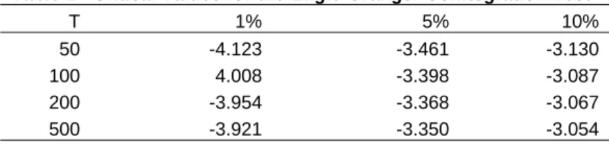
The following table provides a the critical values for the Engle-Granger Cointegration Test:

5% Significance Level for CRDW Statistic for T=50

Table 1 - Critical Values for the Engle-Granger Cointegration Test

T 1% 5% 10%

50 -4.123 -3.461 -3.130 100 4.008 -3.398 -3.087 200 -3.954 -3.368 -3.067 500 -3.921 -3.350 -3.054 The critical values are for cointegrating relations estimated using the Engle-Granger methodology. Source: MacKinnon (1991)

The Engle-Granger Two-Stage Procedure

The earliest procedure developed to explore the relationship between ECM models and cointegration was due to Engle and Granger in the mid-1980s.

1. Establish the Order of Integration of the Variables

Pre-test the variables for their order of integration using, for example, F-tests, DF and ADF tests. It is argued by some that establishing the order of integration in a pre-testing framework may be somewhat misleading. What is ultimately important is whether a combination of variables are cointegrated or not, and this could be achieved through combinations of subsets being I(1) rather than individual series being I(1). It should be noted that some econometricians feel this first step is redundant. However, if all the variables are integrated of order zero, and are thus stationary, it

(26)

is not necessary to proceed any further as standard estimation techniques can be used. The inclusion of variables with different orders of integration may lead to an „unbalanced‟ equation. It might be useful to think of data transformations that transform I(2) variables into I(1) variables. For instance, nominal wages and prices are sometimes found to be I(2) but real wages are generally found to be I(1). One has to be cautious here, however, and, given the weak power of the tests, it may be useful to proceed with caution if the evidence is marginal one way or the other.

2. Estimate the Long-Run Relationship between the Levels Variables

Estimate the following equation using OLS

t t t

y    x u (16)

The following estimates are obtained:

t t t

y   x u (17)

t t t

u   y  x

Retrieve the estimated residuals, which we will defines as ut. Establish whether the residuals are stationary using, for example, DF, ADF or the CRDW tests. In the former two cases, the McKinnon tables could be used to compute the relevant critical values. If the tests indicate that the residuals are stationary, proceed to the next step. This suggests that y and t x are t

cointegrated. Again, if the results are marginal (one way or the other), it is advisable to proceed to the next stage, as this stage offers an additional framework for testing for cointegration.

(27)

Error Correction Mechanism

Cointegration refers to the study of the possible dynamic relationship between n series where one or more have unit roots (are not stationary). The purpose of cointegration analysis is to test whether a linear combination of variables having unit roots is in fact stationary. If this position is fulfilled then it can be concluded that there exists an equilibrium relationship among a set of non-stationary variables, which would imply that their stochastic trends must be linked. Since the trends of cointegrated variables are linked, the dynamic paths of such variables must be linked to the current deviation from the equilibrium relationship. Error correction model looks at this important relationship between the change in the variable and the deviation from the equilibrium. The formal analysis of cointegration, as introduced by Engle and Granger (1987), begins by variables in long-run equilibrium when:

1 1xt 2 2xt nxnt 0

        (18)

If we define  



₁,  , _n



and x_t 



x1,  , x_n



‟ then the long-run equilibrium would imply that βxt = 0. For equilibrium to be meaningful, it must be the case that any deviation from

long-run equilibrium (the equilibrium error et = βxt) must be stationary. Engle and Granger

(1987) provide the following definition of cointegration:

The components of the vector xt



x₁_t,  , x_nt



‟ are said to be cointegrated of order d, b, denoted by xt~ CI d b



,



1. All components of xt are integrated of order d.

2. There exist a vector  



1,  , n



such that linear combination βxt is integrated of order (d – b), where b > 0. β is cointegrating vector.

An important point necessary to note about the definition is that all variables in the model must be integrated of the same order. If all series are not integrated of the same order, they cannot be cointegrated and therefore, there cannot be a long run relationship between these series.

(28)

Error Correction Model is a step forward to determine how variables are linked together. The causal flows that must exist in any cointegrated system are revealed during the second stage of cointegration modeling, the building of an error correction model (ECM). This is a dynamic model based on correlations of returns but with the constraint that short run deviations from the long-run equilibrium will eventually be corrected.

In the simplest case that there are two cointegrated log price series x and y the ECM takes the form:





( ) ( ) 1 1 1 11 12 1 1 p q i i t y t t t i t i yt i i y   y_ x_ a y_ a x_ e       



 



  (19)





( ) ( ) 1 1 1 21 22 1 1 p q i i t x t t t i t i xt i i x   y_ x_ a y_ a x_ e       



 



 

Where the dynamic structure is captured by the difference terms, while the error correction term captures the levels (long-run) information.

If the variables are cointegrated, the residuals from the equilibrium regression can be used to estimate the error-correction model and analyze the long-run and short-run effects of the variables as well as to see the adjustment coefficients, which the coefficient of the lagged residual terms of the long-run relationship identified in cointegration process.

The intuition behind the error-correction model (ECM) is that long run errors have to be corrected in the short-run dynamics such that the process can move closer to its long run target. The ECM is important and popular for many reasons. Firstly, it is a convenient model measuring the correction from disequilibrium of the previous period which has a very good economic implication. Secondly, since ECMs are formulated in terms of the first differences, which typically eliminate the trends from the variables involved, they can play an important role dealing with potential problems leading to spurious regressions. A third very important advantage of the ECM‟s is the ease with which they can fit into the general-to-specific approach to econometric modeling, which is in fact a search for the most parsimonious ECM model that

(29)

disequilibrium error term is a stationary variable. The fact that the two variables are cointegrated implies that there is some adjustment process which prevents the errors in the long-run relationship becoming larger and larger. Engle and Granger have shown that any cointegrated series have an ECM representation. This is very useful when it is wished to test and incorporate both the economic theory relating to the long-run relationship between variables, and short-run disequilibrium behaviors.

2.2 Data

The database for this research is based on the Istanbul Stock Exchange's (ISE) most liquid 50 stocks between the periods 2003 and 2007 end-June.

We divided the data series into two parts: One part for modeling and the other for back testing. The first part of the data includes closes between January 2003 and December 2005. The back testing period is till end-June of 2007 (January 2006-June 2007).

The data summary is given in the Table below:

Number of Sectors Number of Selected Stocks Number of Observations Total Number of Observations

17 50 1,125 56,250

* Out of Stocks from ISE50

* The data for the research is based on the 50 most liquid stocks from Istanbul Stock Exchange between the periods of January 2003 and June 2007

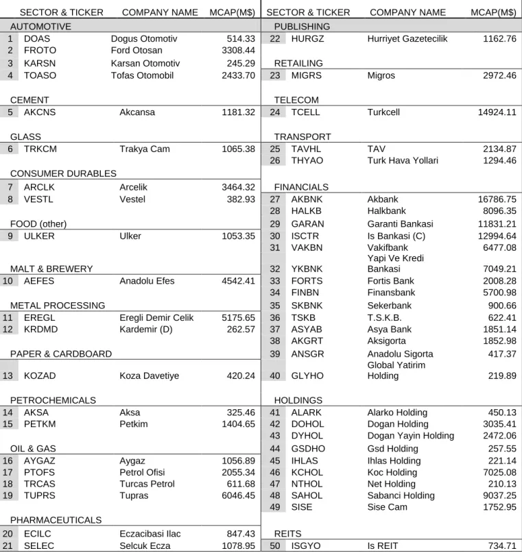
All calculations in this research were updated on a daily basis from the data provider, Reuters. A general list of the stocks, their company names, tickers and floating market capitalizations are given on a Table 3 as of June 29, 2007. All of the model system was designed with Visual Basic Application in Microsoft Excel software and all steps are automated.

(30)

SECTOR & TICKER COMPANY NAME MCAP(M$)

AUTOMOTIVE PUBLISHING

1 DOAS Dogus Otomotiv 514.33 22 HURGZ Hurriyet Gazetecilik 1162.76

2 FROTO Ford Otosan 3308.44

3 KARSN Karsan Otomotiv 245.29 RETAILING

4 TOASO Tofas Otomobil 2433.70 23 MIGRS Migros 2972.46

CEMENT TELECOM

5 AKCNS Akcansa 1181.32 24 TCELL Turkcell 14924.11

GLASS TRANSPORT

6 TRKCM Trakya Cam 1065.38 25 TAVHL TAV 2134.87

26 THYAO Turk Hava Yollari 1294.46

CONSUMER DURABLES

7 ARCLK Arcelik 3464.32 FINANCIALS

8 VESTL Vestel 382.93 27 AKBNK Akbank 16786.75

28 HALKB Halkbank 8096.35

FOOD (other) 29 GARAN Garanti Bankasi 11831.21 9 ULKER Ulker 1053.35 30 ISCTR Is Bankasi (C) 12994.64

31 VAKBN Vakifbank 6477.08

MALT & BREWERY 32 YKBNK

Yapi Ve Kredi

Bankasi 7049.21 10 AEFES Anadolu Efes 4542.41 33 FORTS Fortis Bank 2008.28

34 FINBN Finansbank 5700.98

METAL PROCESSING 35 SKBNK Sekerbank 900.66 11 EREGL Eregli Demir Celik 5175.65 36 TSKB T.S.K.B. 622.41 12 KRDMD Kardemir (D) 262.57 37 ASYAB Asya Bank 1851.14

38 AKGRT Aksigorta 1852.98

PAPER & CARDBOARD 39 ANSGR Anadolu Sigorta 417.37

13 KOZAD Koza Davetiye 420.24 40 GLYHO

Global Yatirim

Holding 219.89

PETROCHEMICALS HOLDINGS

14 AKSA Aksa 325.46 41 ALARK Alarko Holding 450.13 15 PETKM Petkim 1404.65 42 DOHOL Dogan Holding 3035.41 43 DYHOL Dogan Yayin Holding 2472.06 OIL & GAS 44 GSDHO Gsd Holding 257.55 16 AYGAZ Aygaz 1056.89 45 IHLAS Ihlas Holding 221.14 17 PTOFS Petrol Ofisi 2055.34 46 KCHOL Koc Holding 7025.08 18 TRCAS Turcas Petrol 611.68 47 NTHOL Net Holding 210.13 19 TUPRS Tupras 6046.45 48 SAHOL Sabanci Holding 9037.25

49 SISE Sise Cam 1752.95

PHARMACEUTICALS

20 ECILC Eczacibasi Ilac 847.43 REITS

21 SELEC Selcuk Ecza 1078.95 50 ISGYO Is REIT 734.71

(31)

Although, the Float Market Capitalization amounts were not directly used in the modeling or trading section in this research for simplicity, the numbers for all pairs are provided at the last columns.

2.3 Pairs Selection

The investment strategy we aim at implementing is a market neutral long/short strategy. The strategy implies that we will try to find shares with similar betas, where we believe one stock will outperform the other one in the short term. By simultaneously taking both long and short positions, the beta of the pair approaches zero and the performance generated equals alpha.

The challenge in this strategy is identifying stocks that tend to move together and therefore make potential pairs. Our aim is to identify pairs of stocks with mean-reverting relative prices. To find out if two stocks are mean-reverting, the cointegration test is conducted to the log ratio of the pair. Engle-Granger Cointegration Test procedure was applied to determining the stationary in the log-ratio: 1 2 log – log t t t y  S S (20) 1 t t t y  y_     

In other words, we are regressing Δyt on lagged values of yt. The null hypothesis is that γ=0, which means that the process is not mean reverting.

If the null hypothesis can be rejected on the 90% confidence level, the price is following a weak stationary process and is thereby mean-reverting.

2.4 Trading Rules

In order to execute the strategy, we need a couple of trading rules to follow when to open and when to close a trade. Our basic rule will be to open a position when the ratio of two share prices

(32)

hits the 2 rolling standard deviations and close when the ratio returns to the mean. However, we do not want to open a position a pair with a spread that is wide and getting wider.

This can be partly avoided by the following procedure: We actually want to open a position when the price ratio deviates with more than 2 standard deviations from the 132 days rolling mean. The position is not opened when the ratio breaks the 2 standard deviations limit for the first time, but rather when it crosses it to revert the mean again.

We have an open position when the pair is on its way back again. In summary, we:

- Open position when the ratio hits 2 standard deviations bands for two consecutive times. - Close position when the ratio hits the mean.

Furthermore, there will be some additional rules to prevent us from losing too much money on one single trade. If the ratio develops in an unfavorable way, we will use a stop-loss and close the position as we have lost 10% of the initial size of the position.

We will never keep a position for more than 132 days. There is no reason to wait for a pair to revert fully. The maximum holding period of a position is therefore set to 6 months (132 trading days). This should be enough time for the pairs to revert, but also a short enough time not to lose time value.

A pair trading using spread bets requires simply two transactions where one share is bought and another share, usually in the same sector, is sold short. The spread bet trader who utilizes a pairs trading strategy is simply speculating that one share will out-perform the other, in both an up and down stock market. A pairs trading is therefore not a bet on the overall stock market direction. An example of pairs trading would be buying Garanti Bank (GARAN) and selling short Anadolu Sigorta (ANSGR), buying Fort Otosan (FROTO) and selling short Tofas Otomotiv (TOASO) or Koc Holding (KCHOL) and selling short Sabanci Holding (SAHOL).

The chart below shows Tekstilbank‟s price (TEKTL) minus Sekerbank‟s (SKBNK) as an example, and also takes into account the ratio of the two stock prices as they are not the same.

(33)

0.4 0.6 0.8 1.0 1.2 1.4 1.6 1.8 2.0 Ju l-00 Se p -00 O ct -00 Dec -00 F e b -01 Ap r-01 Ma y -01 Ju l-01 Se p -01 O ct -01 Dec -01 F e b -02 Ap r-02 Ma y -02 Ju l-02 Se p -02 Nov -02 Dec -02 F e b -03 Ap r-03 Ju n -03 Ju l-03 Se p -03 Nov -03 Ja n -04 Ma r-04 Ap r-04 Ju n -04 Au g -04 Se p -04 Nov -04 Ja n -05 Ma r-05 Ap r-05 Ju n -05 Au g -05 Se p -05 Nov -05 Ja n -06 Ma r-06 Ap r-06 Ju n -06 Au g -06 Se p -06 Nov -06 Ja n -07 Ma r-07

The stocks‟ values (SKBNK and TEKST) at the beginning of 2000 were taken as an index level 100 and the graph shows how their prices changed until mid-2007. Both stocks have risen during this period. As a first impression from the spread between stocks, it may be possible to imply a long/short strategy to gain money from these stocks.

But firstly, in order to prove the applicability of long/short strategy, cointegration test was performed and the null hypothesis that asserts the process is not mean reverting was rejected at the 90% confidence level, meaning that the price is following a weak stationary process and is thereby mean-reverting.

The Engle-Granger Cointegration Test was used to determine the stationarity in the log-ratio:









log – log t Y  SKBNK TEKST (21) 1 t t t y  y       Entry Point +2 Stdev -2 Stdev Mean Closing Point

(34)

We are regressing yt on lagged values of y . The null hypothesis is that t  0, which means that the process is not mean reverting.

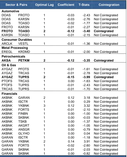
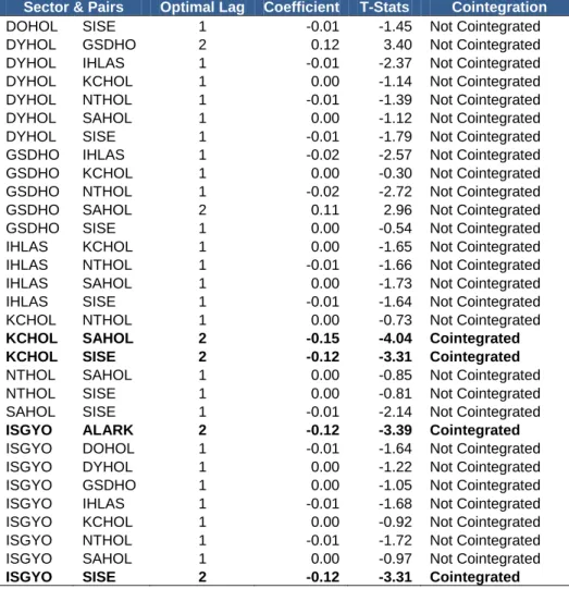
The Engle-Granger Cointegration Test procedure was applied to all of ISE50 stocks within the same sector and the following results are obtained. The optimal lag, Coefficient and T-Stats are also given in the table below. Critical Values for the Engle-Granger Cointegration Test were used to identify the pairs that have cointegration relation and the optimal lags are identified through AIC criteria.

Sector & Pairs Optimal Lag Coefficient T-Stats Cointegration

Automotive

DOAS FROTO 1 -0.03 -2.43 Not Cointegrated DOAS KARSN 1 -0.03 -2.76 Not Cointegrated DOAS TOASO 1 -0.02 -1.77 Not Cointegrated FROTO KARSN 1 -0.01 -2.27 Not Cointegrated

FROTO TOASO 2 -0.12 -3.40 Cointegrated

KARSN TOASO 1 -0.01 -2.15 Not Cointegrated

Consumer Durables

ARCLK VESTL 1 -0.01 -1.36 Not Cointegrated

Metal Processing

EREGL KRDMD 1 -0.01 -2.00 Not Cointegrated

Petrochemicals

AKSA PETKM 2 -0.12 -3.35 Cointegrated

Oil & Gas

AYGAZ PFOTS 1 -0.01 -1.61 Not Cointegrated AYGAZ TRCAS 1 -0.01 -2.78 Not Cointegrated

AYGAZ TUPRS 2 -0.15 -3.99 Cointegrated

PTOFS TRCAS 1 0.00 -1.63 Not Cointegrated PTOFS TUPRS 1 -0.01 -2.43 Not Cointegrated TRCAS TUPRS 1 -0.01 -1.70 Not Cointegrated

Financials

AKBNK GARAN 2 0.12 3.18 Not Cointegrated AKBNK ISCTR 1 0.00 0.29 Not Cointegrated AKBNK YKBNK 3 0.12 3.32 Not Cointegrated AKBNK FORTS 1 -0.01 -2.10 Not Cointegrated AKBNK FINBN 1 0.00 -1.00 Not Cointegrated AKBNK SKBNK 1 0.00 -0.03 Not Cointegrated AKBNK TSKB 1 0.00 -1.37 Not Cointegrated AKBNK AKGRT 1 0.00 -1.05 Not Cointegrated AKBNK ANSGR 1 0.00 -0.79 Not Cointegrated AKBNK GLYHO 1 0.00 0.04 Not Cointegrated GARAN ISCTR 1 0.00 -1.18 Not Cointegrated GARAN YKBNK 2 0.14 3.91 Not Cointegrated GARAN FORTS 1 -0.02 -2.60 Not Cointegrated

(35)

GARAN TSKB 1 -0.02 -2.83 Not Cointegrated GARAN AKGRT 1 -0.01 -2.16 Not Cointegrated

GARAN ANSGR 2 0.11 3.09 Cointegrated

GARAN GLYHO 1 0.00 -0.90 Not Cointegrated ISCTR YKBNK 1 -0.02 -2.43 Not Cointegrated ISCTR FINBN 1 0.00 -0.61 Not Cointegrated ISCTR FINBN 1 -0.01 -1.68 Not Cointegrated ISCTR SKBNK 1 -0.01 -2.01 Not Cointegrated ISCTR TSKB 1 -0.01 -1.51 Not Cointegrated ISCTR AKGRT 1 -0.01 -1.05 Not Cointegrated ISCTR ANSGR 1 -0.01 -1.59 Not Cointegrated ISCTR GLYHO 1 -0.01 -1.55 Not Cointegrated YKBNK FORTS 1 0.00 -0.31 Not Cointegrated YKBNK FINBN 1 0.00 -0.87 Not Cointegrated YKBNK SKBNK 1 -0.02 -2.44 Not Cointegrated YKBNK TSKB 1 0.00 -0.97 Not Cointegrated YKBNK AKGRT 1 0.00 -0.60 Not Cointegrated YKBNK ANSGR 1 0.00 -0.89 Not Cointegrated YKBNK GLYHO 1 -0.01 -1.94 Not Cointegrated FORTS SKBNK 1 -0.01 -1.41 Not Cointegrated FORTS SKBNK 1 0.00 -0.33 Not Cointegrated

FORTS TSKB 2 -0.12 -3.40 Cointegrated

FORTS AKGRT 1 -0.01 -1.95 Not Cointegrated FORTS ANSGR 1 -0.01 -1.48 Not Cointegrated FORTS GLYHO 1 0.00 -0.45 Not Cointegrated FINBN SKBNK 1 0.00 -0.73 Not Cointegrated FINBN TSKB 1 -0.01 -1.77 Not Cointegrated FINBN AKGRT 1 -0.01 -2.15 Not Cointegrated FINBN ANSGR 1 -0.01 -1.75 Not Cointegrated FINBN GLYHO 1 0.00 -0.87 Not Cointegrated SKBNK TSKB 1 0.00 -0.76 Not Cointegrated SKBNK AKGRT 1 0.00 -0.89 Not Cointegrated SKBNK ANSGR 1 0.00 -1.03 Not Cointegrated

SKBNK GLYHO 1 -0.03 -3.54 Cointegrated

TSKB AKGRT 1 -0.01 -2.48 Not Cointegrated TSKB ANSGR 1 -0.02 -2.70 Not Cointegrated TSKB GLYHO 1 -0.01 -1.56 Not Cointegrated

AKGRT ANSGR 1 -0.02 -3.17 Cointegrated

AKGRT GLYHO 1 0.00 -0.72 Not Cointegrated ANSGR GLYHO 1 -0.01 -1.16 Not Cointegrated

Holdings & REITS

ALARK DOHOL 1 0.00 -1.43 Not Cointegrated ALARK DYHOL 1 0.00 -1.22 Not Cointegrated ALARK GSDHO 2 0.10 2.75 Not Cointegrated ALARK IHLAS 1 0.00 -1.78 Not Cointegrated

ALARK KCHOL 2 -0.16 -4.29 Cointegrated

ALARK NTHOL 1 0.00 -1.33 Not Cointegrated

ALARK SAHOL 2 -0.15 -4.00 Cointegrated

ALARK SISE 2 -0.15 -4.12 Cointegrated

DOHOL DYHOL 1 -0.01 -2.09 Not Cointegrated DOHOL GSDHO 1 -0.01 -1.86 Not Cointegrated DOHOL IHLAS 1 -0.01 -2.31 Not Cointegrated DOHOL KCHOL 1 0.00 -1.03 Not Cointegrated DOHOL NTHOL 1 -0.02 -2.41 Not Cointegrated DOHOL SAHOL 1 0.00 -1.07 Not Cointegrated

(36)

DOHOL SISE 1 -0.01 -1.45 Not Cointegrated DYHOL GSDHO 2 0.12 3.40 Not Cointegrated DYHOL IHLAS 1 -0.01 -2.37 Not Cointegrated DYHOL KCHOL 1 0.00 -1.14 Not Cointegrated DYHOL NTHOL 1 -0.01 -1.39 Not Cointegrated DYHOL SAHOL 1 0.00 -1.12 Not Cointegrated DYHOL SISE 1 -0.01 -1.79 Not Cointegrated GSDHO IHLAS 1 -0.02 -2.57 Not Cointegrated GSDHO KCHOL 1 0.00 -0.30 Not Cointegrated GSDHO NTHOL 1 -0.02 -2.72 Not Cointegrated GSDHO SAHOL 2 0.11 2.96 Not Cointegrated GSDHO SISE 1 0.00 -0.54 Not Cointegrated IHLAS KCHOL 1 0.00 -1.65 Not Cointegrated IHLAS NTHOL 1 -0.01 -1.66 Not Cointegrated IHLAS SAHOL 1 0.00 -1.73 Not Cointegrated IHLAS SISE 1 -0.01 -1.64 Not Cointegrated KCHOL NTHOL 1 0.00 -0.73 Not Cointegrated

KCHOL SAHOL 2 -0.15 -4.04 Cointegrated

KCHOL SISE 2 -0.12 -3.31 Cointegrated

NTHOL SAHOL 1 0.00 -0.85 Not Cointegrated NTHOL SISE 1 0.00 -0.81 Not Cointegrated SAHOL SISE 1 -0.01 -2.14 Not Cointegrated

ISGYO ALARK 2 -0.12 -3.39 Cointegrated

ISGYO DOHOL 1 -0.01 -1.64 Not Cointegrated ISGYO DYHOL 1 0.00 -1.22 Not Cointegrated ISGYO GSDHO 1 0.00 -1.05 Not Cointegrated ISGYO IHLAS 1 -0.01 -1.68 Not Cointegrated ISGYO KCHOL 1 0.00 -0.92 Not Cointegrated ISGYO NTHOL 1 -0.01 -1.72 Not Cointegrated ISGYO SAHOL 1 0.00 -0.97 Not Cointegrated

ISGYO SISE 2 -0.12 -3.31 Cointegrated

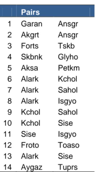
14 pairs have cointegration relation at 90% significance level for the testing period, January 2003 - December 2005.

(37)

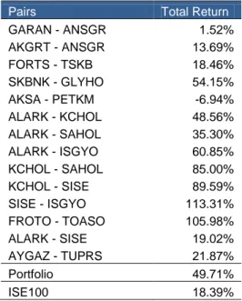
Pairs 1 Garan Ansgr 2 Akgrt Ansgr 3 Forts Tskb 4 Skbnk Glyho 5 Aksa Petkm 6 Alark Kchol 7 Alark Sahol 8 Alark Isgyo 9 Kchol Sahol 10 Kchol Sise 11 Sise Isgyo 12 Froto Toaso 13 Alark Sise 14 Aygaz Tuprs

Pairs trading is better suited to when we have a view over a week or two, perhaps even longer. Everyday pairs trading is often not the way to go because relationships between stocks in the short term can be somewhat fickle. One of the best times to get involved with pairs is when the markets get volatile and there are some clear imbalances between stocks within the same sector, or even against the index itself. Another way to pairs trading is to trade a stock against the underlying index. For example, buy GarantiBank stock (GARAN) and sell short the underlying ISE100 index, on assumption that whatever way the ISE100 moves, GarantiBank share price is likely to outperform.

2.5 Performance of the Strategy

In this research, Istanbul Stock Exchange's (ISE) most liquid 50 stocks were used between the periods 2003 and 2007 end-June. Only the liquid top 50 stocks included in the research because it is not possible to short all of stocks listed in the Istanbul Stock Exchange. In fact, short selling costs are much higher in Turkey compared with the developed markets. A short sales level fee of 5% per annum was used in this paper. (The rebate rate is between 4% and 5% per annum for large liquid Turkish stocks on the basis of a sample survey of prime brokers.)