The impact of exchange rate volatility on trade flows: An empirical study with a panel data approach

THE IMPACT OF EXCHANGE RATE VOLATILITY ON TRADE

FLOWS: AN EMPIRICAL STUDY WITH A PANEL DATA

APPROACH

HANDE KARABIYIK

108622003

İSTANBUL BİLGİ ÜNİVERSİTESİ

SOSYAL BİLİMLER ENSTİTÜSÜ

EKONOMİ YÜKSEK LİSANS PROGRAMI

ASSOC. PROF. EGE YAZGAN

2010

The Impact of Exchange Rate Volatility on Trade Flows: An

Empirical Study with A Panel Data Approach

Döviz Kurundaki Oynaklığın Ticaret Hacmine Etkisi: Panel Data

Kullanılarak Uygulanan Bir Ampirik Çalışma

Hande Karabıyık

108622003

Tez Danışmanı: Doç. Dr. M. Ege Yazgan

...

Jüri Üyesi:

Doç Dr. Koray Akay

...

Jüri Üyesi:

Doç. Dr. Göksel Aşan

...

Tezin Onaylandığı Tarih

:

Toplam Sayfa Sayısı

: 45

Anahtar Kelimeler (Türkçe)

Anahtar Kelimeler (İngilizce)

1)

Panel Değişkenler

1)

Panel Data

2)

Döviz Kuru Oynaklığı

2)

Exchange Rate Volatility

3)

Ortak Bağlı Etkiler

3)

Common Correlated Effects

4)

Ticaret Hacmi

4)

Trade Volume

Özet

Döviz kurundaki oynaklığın ticaret hacmine etkisini önce dünya ticaret hacminin %70’ini oluşturan 42 ülkeyi kullanarak, ardından bu 42 ülke arasından 16 tane gelişmekte olan ülkeyi seçerek analiz ediyoruz. Bu analiz için panel data yaklaşımını kullanıyoruz. Panel Data yaklaşımlarında sıkça karşılalışan bir sorun olan seriler arası bağlılık varsayımı olmadan da çalışabilen birim kök testi ve tahmin yöntemleri kullanıyoruz. Kullandığımız CD test adı verilen test, seriler arası bağlılık olmadan varsayımı olmadan birim kök hipotezini test etmemizi sağlıyor. Ayrıca aynı şekilde Pesaran(2006)’ın geliştirdiği CCE tahminleri de seriler arası bağlılık varsayımı olmadan, modellerimizi test etmemizi sağlıyor. 16 adet gelişmekte olan ülkenin data setini kullanarak elde ettiğimiz sonuçlara göre, döviz kurundaki oynaklığın ticaret hacmine önemli bir etkisi olduğunu gördük. Fakat 42 ülkenin hepsini modelimizde kullandığımızda önemli bir etki tespit edemedik.

Abstract

We examine the impact of exchange rate volatility on the trade flows of 42 countries, which constitutes the 70% share of the total world trade, and also 16 developing countries. We use a panel data approach, and recently developed panel techniques, namely CD test for the panel unit root test, which is developed by Pesaran (2006) and takes into account the cross section dependence, and common correlated effects (CCE) estimators. We find a significant effect of exchange rate volatility to the trade flows for the 16 developing countries. But the results for 42 heterogeneous countries are not significant.

Acknowledgements

First of all, I would like to express my gratitude to my advisor Assoc. Prof. M. Ege Yazgan for his wisdom, guidance, and extraordinary support in all stages of this work. Without his expertise and never-ending support, it would be impossible for me to complete this study. I am very much indebted to him. Also I owe him a great deal for my further academic studies. I will always remember him with great respect and gratitude.

A special thanks goes to Assoc. Prof. Goksel Asan who is like a father to me for more than five years. Without his support and patience I will not be accomplish any of my goals. I know that he will always be there for us with genuine advices, which will lead our lives to the right directions.

I would also like to thank to the professors in the Economics Department of Istanbul Bilgi University; especially to Koray Akay, Remzi Sanver, İpek Özkal Sanver, Fatma Didin, Ayça Ebru Giritligil, Jean Lainé, Çiğdem Çelik for their support, patience and understanding. And beside the respectful, distinguished professors above, I am also thankful to Metehan Sekban, who had never refused me when I need someone to talk and enlightened me with his ideas and advices.

And also I am really thankful to all other employees of Istanbul Bilgi University for creating this lovely, comfortable, and productive environment. That was such a great experience to complete this study in this environment.

The support from TUBITAK, Istanbul Bilgi University is deeply appreciated.

Last, but not least, the most special thanks goes to my parents and my brother. Up to now I have accomplished my goals thanks to their endless support, love and the ambience they have created for me. Their faith in me, has made me feel safe and comfortable in every difficulties I have encountered.

1

Table of Contents

1. Introduction ... 2

2. Literature on Exchange Rate Volatility and Trade Flows ... 5

2.1 Theory ... 5

2.2 Empricial Evidence ... 7

3. Models and Estimation Methods ... 10

4. Data Definitions and Variables ... 15

5. Volatility ... 19

6. Panel Unit Root Tests ... 22

7. Estimation of Long-run Response of Trade Flows... 26

8. Conclusion ... 31

Appendix: Tables ... 32

2

Section 1

Introduction

After the breakdown of the Bretton Woods system in 1973, the exchange rate became volatile with the cross-border financial transactions. As inflation rate, interest rate and the balance of payments become more volatile in the 1980s and early 1990s, interest rate become more volatile too, since interest rate movements are highly depend on the economic fundamentals mentioned above. The exchange rate movements and their effects on various macroeconomic variables have been studied by policy makers and researchers. The impact of the volatility of the exchange rate on trade flows has been the one which the researchers are mostly interested in. The literature on this issue has both theoretically and empirically mixed results. As mentioned in the Côte’s (1994) empirical literature survey on the subject, “There is no real consensus on either the direction or the size of the exchange rate volatility – trade level relationship. Overall, a larger number of studies find that volatility tends to reduce the level of trade, but when the effect is measured, it is found to be relatively small.” On one hand, a number of studies have argued that exchange rate volatility will impose costs on risk averse market participants who will generally respond by choosing domestic trade to foreign trade, when the exchange rate movements are not fully anticipated. From this point of view when hedging is not possible we would expect that as exchange rate risk increases the trade flows would decrease. Akhtar and Hilton (1984), Coes (1981) provides evidences which corroborate this view. On the other hand some argue that trade benefits from exchange rate volatility or risk. For instance; according to Franke (1992), Giovannini (1998) firms use trade as an option like any other options such as stocks. And the value, hence the demand for trade increases as its risk increases. Also some results in the literature have shown that there is no significant evidence that exchange rate volatility affects trade flows.

The motivation behind the present study is to shed an additional light to the issue in question using a country set apart from the country sets studied before, a panel data set,

3

a wider period, and different estimation methods which are presented in Section 7. We also analyze a set of developing countries, whether the volatility of their exchange rates affects their trade flows, or not. The idea of the separation of developing and developed countries, to analyze the effect of exchange rate volatility on trade flows can be found in the literature. For instance Doganlar (2002) focused on effect of real effective exchange rate volatility on exports, and find negative significant effects. We used a panel data set which will allow us to control the unobservable factors. Panel data is increasingly being used by researchers as its importance, and advantages become clear in recent years. And also theoretically there is considerable improvements in the panel data literature which take into account the heterogeneity and cross section correlation issues. New estimation techniques are developed. Heterogeneity is crucial for our case, because the effect of exchange rate volatility can be different for different countries with respect to their financial market structures and also the effects of common shocks may differ among countries. The source of cross section dependency can be the economy-wide common shocks those effect all cross section units in the same direction. So we are in the need of using the right unit root test which allows cross section dependencies and estimation methods. Luckily the literature on panel data provides useful techniques for us to use. We examined the relationship between exchange rate volatility and trade flows empirically by using a panel data set of 42 countries first and then using a panel data set of 16 developing countries. These 42 countries in the first panel data set, constitute more than 70 % of the world trade together. The estimation is carried out between the period 1981Q1 and 2007Q4. We use two different calculation methods for trade flows. For the first one, we only consider the trade flows between the countries in the panel; for the second, we consider the total trade flows of the countries to the world. To check the robustness of our findings, we employ two different measures of exchange rate volatility which are moving average standard deviation of the logarithm on the real exchange rate and standard deviation of the difference of the logarithm of the real exchange rate as a proxy for exchange rate volatility.

We use the unit root test which fits panels with cross section independence, which is called CD tests developed by Pesaran (2007). Then we estimate the long run

4

relationship between exchange rate volatility and trade flows by using a model which explains the evolution of trade flows by using the variables; real gross domestic product, real exchange rate itself, volatility of real exchange rate. The estimation of the long run relationship is carried out by the method called CCE, common correlated effects, developed by Pesaran (2006). This estimator is consistent under heterogeneity and also there is no need to make the assumption of cross section independence. The details about the estimation methods are explained in Section 3.

Section 2 presents the past literature on the subject. Section 3 introduces the model and the estimation methods; Section 4 explains the source and explanation of the variables used. Section 5 explains the proxies used for the volatility measure. Section 6 presents the unit root test results of the variables we used. Section 7 presents the estimation results of the long run response of trade flows. Section 8 presents the conclusion. The results of the test are presented in the tables in the Appendix.

5

Section 2

Literature on Exchange Rate Volatility and Trade Flows

2.1 The Theory

The literature on the effect of exchange rate volatility on trade volume has begun with the collapse of Bretton Woods system, and introduction of floating exchange rates. After all the theoretical work done, still there is no consensus on this issue.

One of the earliest work is Ethier’s (1973). According to Ethier (1973) the traders are risk averse and they respond negatively to high exchange rate risk, which is proxied by the exchange rate volatility. Because firms’ revenue depends on the future exchange rate, the trade decisions are sensitive to the expectations about exchange rate, hence exchange rate volatility. So exchange rate volatility reduces the level of trade. Similar to the theoretical result of Ethier, according to Hooper and Kolhagen (1978) the exchange rate risk has a negative effect on trade flows. Since the exchange rate at the date of the trade can be different from the exchange rate at the date of payment, this will create an ambiguity on the profits in the future. According to their assumption exchange rate risk for all countries is hard to be hedged, because forward markets are not accessible to all traders. As risk cannot be hedged, traders will choose less risky instruments. Also even if the risk can be hedged, there are costs an limitations of such moves, so traders choose less risky instruments instead of hedging their risky assets. And trade volume decreases. So exchange rate volatility affects the trade flows negatively. In both Ethier’s (1973) work, and Hooper and Kolhagen’s (1978) work traders’ attitudes to risk is crucial to have those results. Some of the other theoretical works which a negative relationship is found between exchange rate volatility and trade are; Clark (1973), Baron (1976), Kenen and Rodrik (1986), Peree and Steinherr (1989), Cushman (1986).

A number of subsequent papers claim that there is a positive relation between trade flows and exchange rate volatility. For instance Franke (1991), Sercu and Vanhulle (1992) develops a model where trade is seen as an option that firms held. An increase in the risk of exchange rates, causes the volatility of profitability of trade to increase, that

6

means trade becomes a risky option. As its risk increases, the value of trade increases. Some other theoretical papers, with a result of positive effect are; Klein (1990), Giovannini (1988), Viaene and de Vries (1992). Vieaene and de Vries (1992) has suggested that exchange rate risk can be passed onto the forward rate, and the effect on trade volume can be ambiguous. Moreover, from the political economy point of view, according to Brada and Méndez (1988) while external shocks are taking place, the free movements of the exchange rate make the adjustment of the balance of payments easier. And also reduces the need of other controls like trade restrictions and capital controls in order to have equilibrium. According to Brada and Méndez (1988) this balance of payments balancing function of exchange rate movements encourages the international trade.

Beside the positive and negative results mentioned above, some works has found that the effect is ambiguous. For instance, De Grauwe (1988) suggested that, the theoretical studies which claim that the exchange rate volatility effects trade flows negatively are based on restrictive assumptions. De Grauwe (1988) takes into account both the substitution effect and the income effect which arises with the increase in the volatility of the exchange rate. The substitution effect leads the trades to decrease the export activities, since they choose to shift their investments to less risky instruments. On the other hand the income effect causes a shift of the resources into the export sector when the expected utility of export revenues declines as a result of the increase in exchange rate risk. If the income effect dominates the substitution effect exchange rate volatility will have a positive impact on export activity. So according to De Grauwe (1988) the final effect of volatility on exports depends on the magnitudes of the income effect and substitution effect.

In summary, the theoretical literature has not got a consensus on the effects of exchange rate volatility on trade flows as mentioned before. So the direction of the relationship between the two becomes an empirical issue.

7

2.2 Empirical Evidence

Similar to the theoretical literature, the empirical literature has also mixed results. Some of the results using different models and different calculation methods for exchange rate volatility are summarized below. Beside the empirical studies, numerous survey studies has been done on the subject. Some of them are; IMF (1984), Côte (1994), McKenzie (1999), Clark, Tamirisa, and Wei (2004). McKenzie (1999) suggests that, “Despite the best efforts of economics, a basic paradox as to the impact of exchange rate volatility on trade flows remains unresolved at both the theoretical and empirical level.” Works on this subject deviate from each other with different choices about the definition of the exchange rate, if it is real or nominal, calculation methods of volatility, number of cross section units, the length of the period chosen, the choice of the variables in the model, different model specifications, and the estimation methods.

In the early empirical literature between early 1980s and mid-1990s, researchers use time series data in their models. For instance Akhtar and Hilton (1984) use German and U.S.’s quarterly data between 1974 and 1981, nominal exchange rates in the study. They used OLS as the estimation method and found a negative relationship. The other researches who used time series data and found negative relationship are; Cushman (1983, 1986), Kenen and Rodrik (1986), Thursby and Thursby (1987), Chowdhury (1993), Bini-Smaghi (1991). Chowdhury (1993) examines the G-7 countries in the context of a multivariate error-correction model between the period 1973 and 1990 and uses real exports as the dependent variable. He finds significant negative relationship. Some of the studies are conducted by using cross sectional data, i.e. Brada and Mendez (1998) find negative impact of exchange rate risk on trade volume, by studying with cross sectional data. Some of the early empirical studies with time-series data come up with the conclusion of positive effects. McKenzie and Brooks (1997) has also studied German – U.S. trade and with nominal exchange rate as the independent variable. By using OLS as the estimation method, they find that there is positive effect between exchange rate volatility and exports. A large portion of the results of the studies suggests the effect of the exchange rate volatility on trade flows is ambiguous, or not significant. Hooper and Kohlhagen (1978), Bailey and Tavlas (1988) and Holly (1995),

8

Lastrapes and Koray (1990), Gagnon (1993) find no significant results. Bailey, Tavlas and Ulan (1987) studied the period between 1962 to 1985, use nominal and real exchange rates, and use the estimation method of OLS. And find no significant coefficients. The difference of the study is that they use export growth instead of exports.

Researchers in this area use different calculation methods for exchange rate volatility. For instance Chowdhury (1993) has used moving sample standard deviation of the growth rate of the real exchange rate, with the order of the moving average of eight, while Kenen and Rodrik (1986) use several volatility measures.

Recent literature covers a wide range of variations of the standard models. Baum and Caglayan (2010) analyzed the effect of exchange rate uncertainty to the bilateral trade volume and also trade volatility. They used 13 countries, hence 143 models and take the periods between 1980 and 1998. They find indeterminate results for the relationship of exchange rate volatility and trade flows, only 30 of the 143 models yielded significant coefficients. But a significant positive relationship between exchange rate volatility and trade volatility. They use GARCH approach as a proxy for volatility. Dell’Ariccia (1999) uses a gravity model to analyze the effects of exchange rate volatility on bilateral trade flows through the use of a panel data from Western Europe. The model includes gross domestic product, distance between two countries, populations as independent variables to the model, and common border, European Union membership, and common language as dummies. He uses different variables as proxies for uncertainty, but all give consistent results. He finds a significant negative effect of exchange rate volatility on international trade. Grier and Smallwood (2007) study a sample of nine developed and nine developing countries, and analyses the effect of foreign income uncertainty and real exchange rate uncertainty to international trade. The study differs from other studies on the subject by the separation of developed and developing countries. They find real exchange rate uncertainty has a negative and significant impact on export growth for six of nine less developed countries, and insignificant impact for developed countries. Chit, Rizov and Willenbockel (2010) study the impact of bilateral real exchange rate volatility on real exports of five emerging East Asian economies. The

9

results provide strong evidence that exchange rate voltility has a negative impact on the exports. As we see the conclusions of the studies which concentrate on emerging economies, supports the hypothesis of the negative impact of exchange rate volatility on trade. Other studies those work with emerging or developing countries and find negative impact are; Arize et al. (2000; 2008), Doğanlar (2002). Other recent studies on the subject, with the result of negative impact of exchange rate volatility on trade flows are; Rose (2000), Clark et al. (2004) and Teneyro (2007), Hook and Boon (2000), Vergil (2002), Lee and Saucier (2005).

Aristotelous (2001) investigated the relationship between exchange rate volatility and exchange rate-regime on the British real exports to the United States between the periods 1889-1999. He finds no significant results. Teneyro (2004), Hwang and Lee (2005) are other studies those find no significant results. Kasman & Kasman (2005) use real exports in their analysis and cointegration and ECM models. They find significant positive effect of exchange rate volatility on trade flows.

Empirical studies have contradictory result similar to the theoretical approaches. The empirical results are, in general, sensitive to the choices of sample period, model specification, form of proxies for exchange rate volatility, and countries considered. The mixed empirical results can be caused by different choices of those variables.

10

Section 3

Models and Estimation Methods

Several models are used to explain how the trade flow demand is constituted in the literature. The economics theory suggests that the income of a country is a major determinant of a country’s trade flows. We use natural logarithm of the GDP of a country as an explanatory variable in all our models. The second explanatory variable is the the natural logarithm of the real exchange rate itself is added to the regression model. And finally of course volatility measure is included in the model. So the models we analyze is constituted of real gross domestic product, real exchange rates, and volatility.

Different choices about which countries to include (42 chosen countries or 16 developing countries), different definitions of variables in the models (we use two different volatility measures, and also two different calculation methods for trade flows) lead us to anaylse six different models in this study. The models will be explained below, in this section, and the variables used in each model will be described in Section 4.

The first model can be expressed as;

1 2 3 1 , 1, 2, ..., ; 1, 2, ..., ; 42(1)

it i i it i i it it

t

f

=

α

+

β

y

+

β

e

_it +

β

v

+

ε

i = N t = T N =

Where all variables except volatility are expressed in natural logarithms. tf is the _it natural logarithm of the sum of exports of country i to other 41 countries included in the panel and imports from the 41 countries in the panel to country i at time t. yit is the

natural logarithm of the real output of country i at time t. e_it is the real exchange rate of country i at time t. v_1it is the first type of volatility measure of country i at time t. The measures for volatility used in this study will be explained in section 5.

11

The second model can be expressed as;

1 2 3 2

,

1, 2, ...,

;

1, 2, ..., ;

42(2)

it i i it i it i it it

i

N t

T N

tf

=

α

+

β

y

+

β

e

+

β

v

+

ε

=

=

=

We use the second type of volatility measure in the second model. The only difference from the first model is this. In this model the volatility variable v is the second type of _2it volatility measure of country i, at time t.

The third model can be expressed as;

1 2 3 1

,

1, 2,...,

;

1, 2,..., ;

16(3)

d d d d

it i i it i it i it it d d

t

f

=

α

+

β

y

+

β

e

+

β

v

+

ε

i

=

N

t

=

T N

=

We also analyze the trade flow demand function of 16 developing countries apart from all other countries. tf stands for the natural logarithm of the trade flows of a _itd developing country i at time t. d

it

y is the natural logarithm of the real output of a

developing country i at time t. And finally e , and _itd v are the real exchange rate and ₁d_it volatility type 1 of a developing country i respectively.

The fourth model can be expressed as;

1 2 3 1

,

1, 2, ...,

;

1, 2,..., ;

42(4)

it i i it i it i it it

i

N t

T N

wt

=

α

+

β

y

+

β

e

+

β

v

+

ε

=

=

=

In this model, we use the data for the total world trade flows of country i, instead of the trade flows between country i and other 41 countries in the model. wt_it

, and v are 1it

variables which stand for the natural logarithm of total world trade flows of country i, at time t, and first type of volatility measure of country i, at time t.

The equation for the fifth model is below; the only difference from the fourth model is the choice of the volatility measure used. We use second type of volatility measure in model 5.

1 2 3 2

,

1, 2,...,

;

1, 2, ..., ;

42(5)

it i i it i it i it it

i

N t

T N

12

The data used sixth model, is again only include 16 developing countries as in Model 3.

d it

wt is the total world trade flow of a developing country i. We use first type of volatility measure as in Models 1, 3, and 4. The equation for the sixth model is expressed as;

1 2 3 1

,

1, 2,...,

;

1, 2,..., ;

16(6)

d d d d

it i i it i it i it it

i

N

d

t

T N

d

wt

=

α

+

β

y

+

β

e

+

β

v

+

ε

=

=

=

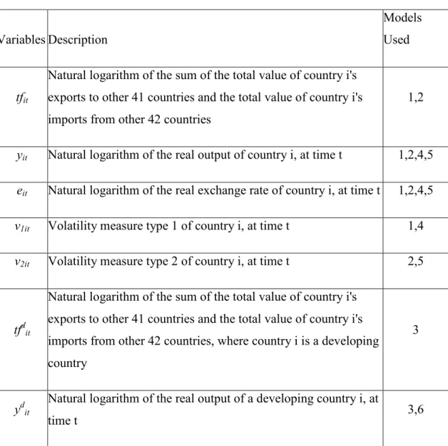
The summary table for the variables used in the models, their descriptions, and the number of models they are used in is below;

Table A: Variables used in the models and their descriptions

Variables Description

Models Used

tfit

Natural logarithm of the sum of the total value of country i's exports to other 41 countries and the total value of country i's imports from other 42 countries

1,2

yit Natural logarithm of the real output of country i, at time t 1,2,4,5

eit Natural logarithm of the real exchange rate of country i, at time t 1,2,4,5

v1it Volatility measure type 1 of country i, at time t 1,4

v2it Volatility measure type 2 of country i, at time t 2,5

tfdit

Natural logarithm of the sum of the total value of country i's exports to other 41 countries and the total value of country i's imports from other 42 countries, where country i is a developing country

3

ydit

Natural logarithm of the real output of a developing country i, at

13

edit

Natural logarithm of the real exchange rate of a developing

country i, at time t 3,6

vdit Volatility measure type 1 of a developing country i, at time t 3,6

wtit

Natural logarithm of the sum of country i's exports to the world

and imports from the world 5

wtdit

Natural logarithm of the sum of country i's exports to the world and imports from the world where country i is a developing country

6

The basics behind the estimation methods used, and the assumptions are explained below. As it is mentioned before, we use CCEMG and CCEP estimation methods developed by Pesaran (2006).

As we see from all Models, the parameter vector; β_i =

₍

β β_i1, _i2,β_i3

₎

′, of the explanatory variables vary over both time and countries and the parameter vector α_i =(

α

_i)′which is deterministic and vary only over time, but not over countries. These two parameter vectors are both allowed to be heterogeneous across countries.

The procedure developed by Pesaran (2006) can account for unobserved common effects. The unobserved common factor effects can be included by assuming the following multi-factor structure,

it i t it

u =γ′f +

ε

(7)

Where f is an _t m ×1vector of unobserved common shocks and

ε

_itare the individual specific (idiosyncratic) errors. Those idiosyncratic errors are assumed to be independently distributed of y_it,p e , and _it, _it f . The common factors _t f can possibly be _t

14

correlated with the explanatory variables. If

ε

_it is stationary and mis a fixed number,

t

f can be stationary of non-stationary.

The long run effects of the explanatory variables to the dependent variable can be assessed by computing the average values of β s. The β matrix can be computed by _i taking the averages of each β equals the expectation of _i β s, denoted by ( )_i Ε βi =β . In

order to compute this expectation we need to assume a random coefficient model,

= + i i β β ω , where IID

(

)

i i ω ω 0, V .

We use two types estimators of the mean value of β . First one is CCEMG (CCE mean group estimator). CCEMG is a simple average of the individual CCE estimators. Second one is a pooled estimator of β which is denoted by CCEP. The second one is preferred when the individual slope coefficients, β , are the same. We can gain _i efficiency by pooling observations over the cross section units when the individual slope coefficients are the same.

The common correlated effects (CCE) estimators are based on the cross section augmented regressions. We show the augmented regression only for Model 1, the augmented regressions for other models can be derived using the same procedure. For the first model, an augmented regression can be shown as;

1 2 3 1 1 2 3 4 1

it it i it i it i it i t i t i t i t it

t

f

=α +β

y

+β

e

+β

v

+d

tf

+d

y

+d

e

+d

v

+υ (8)

Where tf y e_t, _t, _t and v_tare cross section averages of tf_it,y e and _it, _it v at time t. We can _it obtain the CCE estimators simply by applying OLS to Equation (8).

This is important to allow the unobserved factors in the model. In order to show the importance we also estimate the Mean Group (MG) estimators, which are computed simply by running OLS to the models in Equations 1 to 6. These mean group estimators do not allow for cross section dependence. MG estimators are not reliable, since the assumption of cross section independence is not valid for our data set. The test procedures and results for cross section dependence is shown in Section 6.

15

Section 4

Data Definitions and Variables

We use two different sets of data in this paper. First a panel data set of 42 countries over the period between 1981:Q1 to 2007:Q4 is used. The countries used in the panel are; Argentina, Australia, Austria, Belgium, Brazil, Canada, Chile, China, Hong Kong, Denmark, Finland, France, Germany, Greece, Hungary, India, Indonesia, Iran, Ireland, Israel, Italy, Japan, Korea, Malaysia, Mexico, Netherlands, New Zealand, Norway, Peru, Philippines, Portugal, Saudi Arabia, Singapore, South Africa, Sweden, Switzerland, Spain, Thailand, Turkey, United Kingdom, the United States, and Venezuela. Second we use the data set for the 16 developing countries. The developing countries used in the analysis, are chosen by taking into consideration of the report of International Monetary Fund’s World Economic Outlook Report dated October, 2009. The developing countries used in the construction of the panels are; Argentina, Brazil, Chile, China, Hungary, India, Indonesia, Iran, Malaysia, Mexico, Peru, Philippines, South Africa, Thailand, Turkey, Venezuela.

The variables used in this study are trade volume (two different types), exports, real GDP, real Exchange Rate, Consumer Price Index, nominal exchange rate. The details about the data construction process are described below.

For the first type of trade flows, the source of exports and imports data is IMF – Direction of Trade Statistics (DOT). The values of exports and imports are expressed in U.S. dollars. We use nominal trade flows. The trade flow data for country i is computed according to the formula below;

1 1

(

)

n it ijt jit j

tf

−

ex

im

=

=

∑

+

Where exijt is the U.S. dollar value of the exports from country i to country j, imjit is the U.S. dollar value of the imports from country j. j denotes each country in the panel

16

except country i. tf is the sum of country i’s exports to 41 countries in the panel and _it country i’s imports from 41 countries in the panel. There are some country-specific calculation methods, which are described below.

For Belgium, we use the exports and imports data of Belgium-Luxembourg between the period 1981:Q1 and 1996:Q4. And from 1997:Q1 until 2007:Q4 we use the total value of the trade flows of Belgium and Luxembourg. For South Africa, the data of export from any country to South Africa were not available. Because of the missing data, instead of the normal calculation method above, we used the calculation method below;

1 1 ( ) n st sjt jst j t

f

−

im

im

= = ∑ +

Where s is the index for South Africa. The amount of imports from any country to South Africa is used as a proxy for the amount of exports of South Africa to any country.

Another dependent variable which is used in Model 3 is tf . This is the trade flow _itd variable for developing countries. We take the sum of the exports to all 41 countries and imports from all 41 countries. The difference is that, i index in the notation includes only developing countries while j indices in the formula below includes all countries in the panel, regardless of it is a developing country or not.

1 1 ( ) n d d d it ijt jit j

tf

−

ex

im

= = ∑ +

The third dependent variable, which is used in models 4 and 5, is the world trade data for each country. This data is taken from IMF-DOT. For instance Argentina’s world trade flow data period 1981Q1 is the sum of Argentina’s exports to the World and Argentina’s imports from all over the World. This amount is also recorded in U.S. Dollars. The formula for the variable is;

w w

it it it

17

The real GDP data is mostly taken from IMF – International Financial Statistics. The GDP volume with constant prices where 2005 prices equal to 100 is used. Quarterly data were not available for some countries, interpolation is used to derive the quarterly data from annual data for those countries. The interpolation procedure is described in Dees et al (2006) .The countries and the periods (given in the brackets) which we used interpolation for each country are; Argentina (1981:Q1 – 1989:Q4), Brazil (1981:Q1 – 1990:Q4), China (1981:Q1 – 2007:Q4), Greece (1991:Q2 – 1999:Q4), Hungary (1981:Q1 – 1994:Q4), India (1981:Q1 – 1996:Q3), Indonesia (1981:Q1 – 1992:Q4), Iran (1981:Q1- 1994:Q4), Ireland (1981:Q1 – 1996:Q4), Malaysia (1981:Q1 – 1987:Q4), New Zealand (1981:Q1 – 1981:Q4), Saudi Arabia (1981:Q1 – 2007:Q4), Thailand (1981:Q1 – 1992:Q4), Turkey (1981:Q1 – 1986:Q4), Venezuela (1981:Q1 – 2007:Q4). GDP volume with constant prices data for some countries are not available in IMF-IFS. Namely, we use the statistics at Banco Central de Brasil for the GDP data of Brazil, OECD for Indonesia, Philippine Institute for Development for Philippines, and Datastream for Singapore. For Philippines and Singapore we could find GDP data only in the 1995 and 2000 constant prices format respectively, so we convert them to 2005=100 prices. Some countries’ GDP data are needed to be seasonally adjusted in order to remove the seasonal component of the series. Seasonal adjustment was performed with E-Views, using the U.S. Census Bureau’s X12 program. The countries for which we use seasonally adjusted GDP are; Argentina, Austria, Belgium, Brazil, Hong Kong, Chile, Denmark, Finland, Greece, Hungary, India, Indonesia, Iran, Ireland, Israel, Korea, Malaysia, Norway, Philippines, Portugal, Sweden, Thailand, and Turkey. The exchange rate data used in the model is the real exchange rate, obtained by using nominal exchange rates and consumer price indexes of each country. The formula used in calculating the real exchange rate data for each country is;

us it t it

e

cpi

cpi

×

18

Where eit is the nominal exchange rate of country i in domestic currency per US dollars at time t, cpius is the consumer price index of the US at time t, and cpi is the consumer _it price index of country i at time t.

The nominal exchange rate data, are all taken from IMF-IFS. Nominal exchange rate of country i is defined as period average value of national currency of country i per U.S. Dollars. For the countries which adopted Euro, the conversion rates from their original currency to euro are used, with the base of U.S. Dollar value of Euro at 2000. We have extracted the data over the period 1978:Q1 – 2007:Q4, in order to use them in the calculation of volatility. The measures and calculation methods of volatility will be explained in Section 5.

The Consumer Price Index Data are taken from IMF-IFS except China. CPI data for China is taken from Dees et al. (2006) up to 2003, the remaining data were completed by using the growth rates published by IFS. The base year is 2005 for all countries. (2005=100). Germany’s CPI data is computed by using 1991 prices of both Unified Germany and West Germany as a base and then convert them to 2005 = 100 prices. The data for developing countries is constructed by deleting the cross sections from the panels which are not included in the list of 16 developing countries. So the data for 16 developing countries has the same properties with the data for 42 countries.

19

Section 5

Volatility

Exchange rate volatility is defined as the risk associated with unexpected movements in the exchange rate. Several different exchange rate volatility measures have been used in the literature. E.g., average of absolute changes, standard deviations, moving average standard deviations, GARCH. Chowdhury (1993) uses moving sample standard deviation of the growth rate of the real exchange rate with the order of moving average 8. This measure is used in many studies. Some of them are; Kenen and Rodrik (1986), Koray and Lastrapes (1989), Lastrapes and Koray (1990), Arize et al., Aristotelous (2001). This measure captures the temporal variation in the absolute magnitude of changes in real exchange rates over time. Baum, Caglayan and Ozkan (2004) utilize daily spot exchange rates to compute one month-ahead exchange rate volatility from the intra-monthly variations in the exchange rate. This high frequency approach to obtain volatility is used by some other researchers, namely; French et al.(1987), Klaassen (1999). Dell’Ariccia (1999) uses three different types of volatility; the standard deviation of the first difference of the natural logarithmic exchange rate, the sum of the squares of the forward errors, and the percentage difference between the maximum and the minimum of the nominal spot rate. Conditional variance (ARCH/GARCH) is used in most of the recent studies on the subject, i.e. Grier and Smallwood (2007), Fang,Lai and Miller (2009), Sauer and Bohara (2001), Clark, Tamirisa and Wei (2004). The generalized autoregressive conditional heteroscedasticity (GARCH) method assigns different weights (generally decreasing), while computing the standard deviation of the data. And allows for volatility clustering such that large variances in the past generate large variances in the future. Chit, Rizov, Willenbockel (2010) also use three measure of exchange rate volatility; the standard deviation of the first difference of the log real exchange rate, the moving average standard deviation (MASD) of the quarterly log of bilateral real exchange rate which is the same as what Chowdhury (1993) uses, and the conditional volatilities of the exchange rates estimated using GARCH model.

20

We employ two measures of volatility, first the standard deviation of the difference of the natural logarithm of the real exchange rate, second moving average standard deviation of the logarithm of the real exchange rate.

To compute the first type of measure for exchange rate volatility, we use the formula below; 2 1 1 ( ) 1 m it it it t m

V

e

e

= = ∑ ∆ − ∆ −

Where eit is the real exchange rate. This is the standard deviation of the percentage change of the exchange rate, the proxy can take the value of zero if exchange rate follows a constant trend, and gives larger weights to extreme observations. If the exchange rate follows a constant trend, it means that it can be perfectly anticipated, and the volatility measure has to be zero.

The second measure is the moving average standard deviation, which is commonly used in the literature. The main characteristic of this measure is that it implies a high persistence of real exchange rate shocks and so considerable serial correlation in risk; it accounts for periods of high and low exchange-rate uncertainty, since it’s time varying exchange rate volatility. The formula we used in calculating the measure is;

1/2 2 2 1 2 1 (1 / ) (ln ln ) m it it i it i i m

V

e

_{+ −}

e

_{+ −} = =



_

∑ −



_





Where eit is the real exchange rate and m is the order of the moving average. K. Aristotelous (2001) has chosen m equal to 4, Chowdhury (1993) has chosen m equal to 8, following Chowdhury we also chose m=8. The choice of the weighting scheme can be seen important but it has been shown that the results are not very sensitive to the choice of the weighting schemes (see Chowdhury (1993)).

There are some deviations from the formula above for three countries, which are Brazil, China, Hong Kong. The nominal exchange rate series and consumer price index series for Brazil start from 1980Q1. So we cannot compute the Real Exchange Rate of Brazil until the period 1980Q1. We also cannot compute the real exchange rate of China until

21

the period 1980Q1, since the consumer price index data were missing. Also for Hong Kong the series for CPI starts 1980Q4. It is obvious that the series should start at least at 1979Q2, to compute the volatility for 1981Q1 with a moving average order of 8 periods. We use changing moving average orders in order to use all available data. The moving average order increases as the data we use to compute the volatility becomes available, and it becomes fixed when we reach the moving average order of 8. For instance for Brazil, in order to compute the volatility at 1981Q1, we use a order of moving average of 4, and to compute the volatility at 1981Q2 we use moving average order of 5. We use a moving average order of 6 to compute the 1981Q3 volatility, 7 to compute the 1981Q4 volatility, and 8 to compute 1982Q1 volatility, and hereafter the moving average order is 8 for the volatility computations for all other periods.

We use the first type of volatility in the analysis for developing countries in order not to complicate the analysis by increasing the number of results. To obtain the panel data for volatility for developing countries, we just delete the series for the countries which are not in the developing countries list.

22

Section 6

Panel Unit Root Tests

We analyze the time series properties of the variables used in the model by applying panel unit root tests. Most of the panel unit root tests in the literature require the assumption of cross section independence. Irandoust, Ekblad and Parmler (2006) used a test generated by Im et al. (2003), which is based on a standard Dickey-Fuller test. Their claim is the test generated by IM et al. (2003) has an improved power. Chit, Rizov and Willenbockel (2010), also used IPS test (Im, Pesaran and Shin, 2003) and the Hadri LM test (Hadri, 2000). IPS test is based on the mean of individual unit root statistics and has a null hypothesis of all series in the panel are non-stationary against the alternative hypothesis of a fraction of the series in the panel being stationary. So for large T, IPS test has high power but, also the test has a risk of a conclusion of stationarity even when most of the series in the panel is non-stationary. The tests mentioned above require the assumption of cross-section independence in order to be valid. Other panel data unit root tests in the literature which assume cross-section independence are the tests developed by; Choi (2001), Levin et al. (2002), Maddala and Wu (1999), Shin and Snell (2002). The assumption of the existence of cross section independence is not a realistic assumption. In this study we first show the strength of the cross section dependence by computing the cross correlations of the residuals from ADF(p) regressions, and test the significance of the dependence with CD test. And show how unrealistic the cross-section independence assumption is. And then test whether the panels has a unit root or not by using CIPS test developed by Pesaran (2007), which is a test gives consistent results even if the there is cross- section dependence.

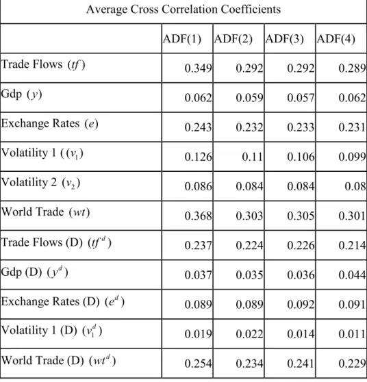
We first show the evidence on the extent of cross section dependence of the residuals from ADF(p) regressions of the variables used. The evidence of cross section correlation is presented with ADF(p) regressions of trade flows ( tf ), real output ( y ), real exchange rate (e), volatility type 1 which defined as the natural logarithm of the real exchange rate (v ), volatility type 2 which is defined as the moving average ₁

23

standard deviation of the logarithm of the real exchange rate (v ), total world trade ₂ flows of the countries in the panel ( wt ) and trade flows of developing countries ( d

tf ), real output of developing countries ( d

y ), real exchange rates of developing countries

(ed), and volatility type one data for developing countries (v ) and world trade across ₁d 16 developing countries (wtd), are summarized in Table 1 in the Appendix.

For each lag of ADF tests, i.e. p=1;2;3 and 4, we also compute average estimates of the pair-wise correlations of the residuals, which is denoted by ρ . For trade flows, real ˆ

exchange rates, and world trade for all 42 countries, and trade flows and world trade for developing countries _{ρ is estimated to be around 30%, 24%, 34%, 22%, and 23%} ˆ

respectively, while for real output for both 42 countries and 16 developing countries, it is reasonably lower and the estimate is around 6%, and 4% respectively. Normally, we would expect these estimates to be higher because of possible international business cycles among 42 countries and also 16 developing countries. The low level of estimated correlations can be caused by the heterogeneity of the countries chosen. The average estimate of the pair-wise correlations of the residual, _{ρ of the exchange rate} ˆ

variable for 16 developing countries is around 9%. This low value of _{ρ of can be} ˆ

explained by the instability of the financial markets of developing countries. The _ρ ˆ

value for all three different volatility variables is also low. Volatility 1 for all 42 countries has a _{ρ value of 12%, volatility 2 for 42 countries has a} ˆ _{ρ value of 8%, and} ˆ

volatility 1 for 16 developing countries has a _{ρ value of 1%.} ˆ

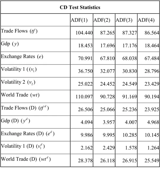
To test the significance of these correlations we use a Cross-section Dependence (CD) test of error cross section dependence which is developed by Pesaran (2004). This test is also emphasized by Holy et al. (2008). The CD test does not require an a priori specification of a connection matrix and is applicable to a variety of panel data models, including stationary and unit root dynamic heterogeneous panels with structural breaks, with short T and large N. The CD test is based on an average of the pair-wise correlations of the OLS residuals from the individual regressions in the panel, and tends to a standard normal distribution as N → ∞. The CD test statistics, reported in table 2

24

in the appendix, clearly show that the cross correlations are statistically highly significant except the volatility for 16 developing countries. Since most of the variables used in the model are significantly cross sectionally correlated, this invalidates the use of panel unit root tests that do not allow for error cross section dependence.

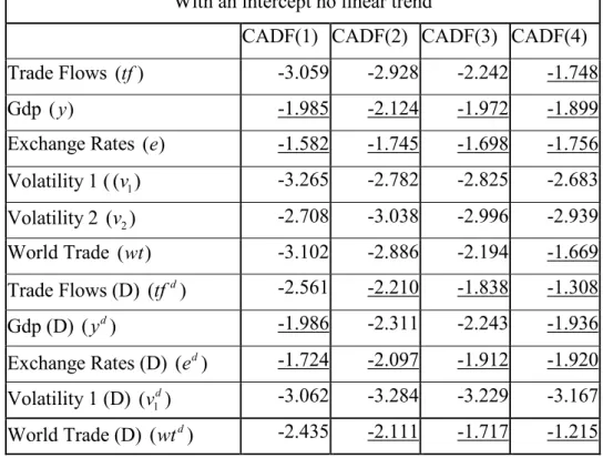
Since the cross section dependence is highly significant in the panel we choose to use the panel unit root tests which are valid when there is cross section dependence. Recently, a number of panel unit root tests that allow for possible cross section dependence in panels have been proposed in the literature, some of them are mentioned above. In this paper, the simple test proposed by Pesaran (2007), which is denoted as the CIPS test, is employed. The test is a simple alternative to ADF test. CIPS test follows common correlated effects (CCE) approach and eliminate the cross section dependence by augmenting the ADF (CADF) regressions with cross section averages as in the formula below;

1 1 N i i CIPS CADF N = = ∑

Where CADFi is the cross-sectionally augmented Dickey-Fuller statistic for the i-th cross sectional unit. (See Pesaran, 2007 for details)

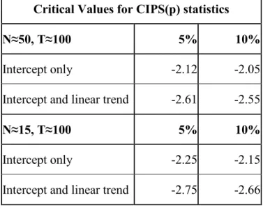
We ran all the variables first without a linear trend but with intercept and then with linear trends and intercepts. To capture the trend in real output for both 42 countries data and 16 developing countries data, we check only the result with the trend and intercept. The CIPS test statistics are shown in Table 3. The significance levels are indicated in table 5.

The test statistics which are above both 5% and 10% critical levels (leads to the conclusion of not rejecting the null hypothesis of unit root) are underlined in the table. For the real output and real exchange rate for all countries and also for developing countries, the unit root hypothesis cannot be rejected, in the case of a linear trend. It’s rejected for the trade volume data of all 42 countries for the 1st, 2nd, 3rd augmentation orders in the case of no linear trend and also in the case of a linear trend. The null hypothesis of unit root for the trade flow data and also world trade data of 16

25

developing countries is rejected only for the first augmentation in the case of a linear trend and also in the case of no linear trend. It seems that the world trade data for 42 countries has a unit root only for the augmentation orders 1st 2nd in the case of a linear trend. For both measures for volatility for all countries and also for developing countries, the null hypothesis of unit root is rejected. And also we can say that world trade data for developing countries has a unit root. Pesaran’s CIPS test for unit root convincingly indicates that, real output, real exchange rate and trade flows data for developing countries has a unit root. And all volatility measures, trade flows for all countries used, does not have unit root.

Table 4 shows the CIPS test statistics of the differences of the variables, which has a unit root. The table shows that the unit root hypothesis is rejected for the differences of real output, real exchange rate, trade flows of developing countries, world trade of developing countries, real output of developing countries, real exchange rate of developing countries. Therefore, there is strong evidence that supports that the variables denoted above follow an I(1) process.

26

Section 7

Estimation of long-run response of trade flows

We estimate a long-run trade flow demand model by using the variables; real output, real exchange rate, and exchange rate volatility for various data sets which lead us to analyze 6 different models. The long-run response of trade flows to real exchange rate and output is estimated by using 3 different estimators (MG, CCEMG, CCEP). The estimation methods are explained in section 3. MG, CCEMG and CCEP estimators are developed by Pesaran (2006). The results obtained by using the procedure developed by Pesaran (2006) are in table 6.1, 6.2, 6.3, 6.4, 6.5, and 6.6 in the Appendix.

We also estimate the coefficients when there is a linear time trend among our repressors. Since the coefficient of the time trend is highly significant in our entire model set, we consider the results when the time trend is present. The calculated t-values for the time trends can be seen from the table below;

Model 1 Model 2 Model3 Model 4 Model 5 Model 6 t(NP) 4.972 4.49 2.739 5.379 4.827 2.701

The CD test statistics in the tables indicates the calculated t-values for the test of cross section dependence, with the null hypothesis of no error cross section dependence. The high CD test statistics for each 6 model obtained by using MG estimators tells us that the MG estimators are biased, since the assumption of no cross section dependence is used in the calculation of the estimators. The CCEP estimator is preferred, when the individual slope coefficients are the same. The CCEP estimator is more efficient than the CCEMG estimator. But the assumption of slope homogeneity is not valid for our data set. So we prefer CCEMG estimators, but we also present the results of MG and CCEP estimators. And also comment on those.

27

First we comment on the effect of output on trade flows. The coefficient

β

₁ of the output varies between 0.847 and 1.52. And they are highly significant for all 6 Models and all 3 estimators namely; MG, CCEMG and CCEP. The t values vary between 4.32 and 17.39. For instance we can say that, considering the first model and CCEMG estimator; one percent increase in an output of a country will cause an increase of 1.45 percent in the trade flows in the long-run. The existence of the output in the trade flow demand function is supported one more time with this empirical study. In other words the output level of a country affects the decisions of agents about trade significantly positively according to the results. The coefficients and their t-values can be found in the Tables 6.1 – 6.6.

The exchange rate itself is also significant in most of our models. The coefficient

β

₂ of the exchange rate is negative for all models. The size of the coefficients strongly depends on the estimation methods. The coefficients are larger when we consider MG or CCEMG estimation methods; it becomes smaller when we use CCEP estimation method. Since the coefficients calculated with the estimation method MG is biased because of the cross section dependence, and the coefficients calculated with the estimation method CCEP is not valid because of the violation of the assumption of homogeneity of the individual slope coefficients we consider the estimation method of CCEMG. For the case of the first model and with CCEMG estimation method, the estimator for

β

₂ equals -0.473. Which means one percent increase in the exchange rate leads 0.473 percent decrease in the trade flows of a country in the long-run. And the t-value of that coefficient is -2.696, which shows us that the coefficient is highly significant. For Model 2; the coefficient equals -0.341 and the t-value is -3.881. This shows us that any change in the exchange rate affects the trade flows significantly negatively in the long-run no matter what kind of calculation method we use for volatility. For Model 3; the coefficient is smaller than the first two models, and it is not significant. The coefficient is -0.062 and the t-value is -0.803. We can say that for developing countries the exchange rate itself is not affecting the trade flows significantly. If we consider the total world trade of the 42 countries as a dependent variable, as we did in models 4 and 5, we see that the coefficient of the exchange rate is

28

significantly negative. The coefficients of the exchange rate are -0.295 and -0.326 respectively for models 4 and 5. And the tvalues for these coefficients are 3.801 and -4.147. For the sixth model, which we consider the world trade flows of 16 developing countries the coefficient is small and also insignificant. We can conclude that in the long-run the exchange rate affects the trade flows of 42 heterogeneous countries, but it does not affect the trade flows of developing countries significantly.

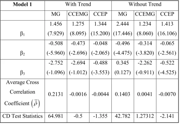
To analyze the effect of the volatility of the exchange rate to the trade flows of the countries is our main purpose. The coefficients we estimated can be seen from the Tables 6.1 to 6.6. For the first Model; we use the first type of volatility which is the standard deviation of the difference of the natural logarithm of the real exchange rate. The estimated coefficients equal to -2.752, -2.694 and -4.888 and the related t-values are -1.096, -1.012 and -3.553. We see that for the estimation methods MG and CCEMG the effect of volatility to the trade flows is not significant. It becomes significant when we use the estimation method of CCEP but this method is not valid for our data set. The coefficients are all negative regardless of which estimation method we use. So we can conclude that with the 42 countries panel data the volatility has not got a significant effect on trade flows with the estimation methods of MG and CCEMG. If the first model could be estimated by CCEP we see that all the explanatory variables have significant coefficients. According to this result we could claim that, in the long run if the exchange rate volatility of a country increases by 1 percent, this will cause the country’s trade flows to decrease by 0.131 percent. But the only valid or unbiased result is the result obtained by using CCEMG estimation method. And the estimated coefficient of CCEMG equals -2.694 which is negative as expected but not significant in any critical level.

In the second model we use the second type of volatility which can be defined as moving average standard deviation of the logarithm of the real exchange rate. The dependent variable in the model is the total trade flows between the countries in the panel. The coefficients of the volatility variable in the second model, for three different estimation methods, are; -0.361, 0.263, -0.131 and their respective t-values are; -1.000, 0.843, -2.040. The statistical significance of the estimates depends on the estimation

29

methods we use. The third estimator which is obtained by using CCEP is significant but the others are not significant. In models 1 and 2; we cannot find strong significant estimate of the coefficient of the volatility. As in the whole literature the results we obtained from the regression models depends on the estimation methods. This can be caused by the heterogeneity of the countries we choose to analyze. In order to distinguish the effect of the heterogeneity of the countries to the results, we use 16 developing countries in the Models 3 and 6.

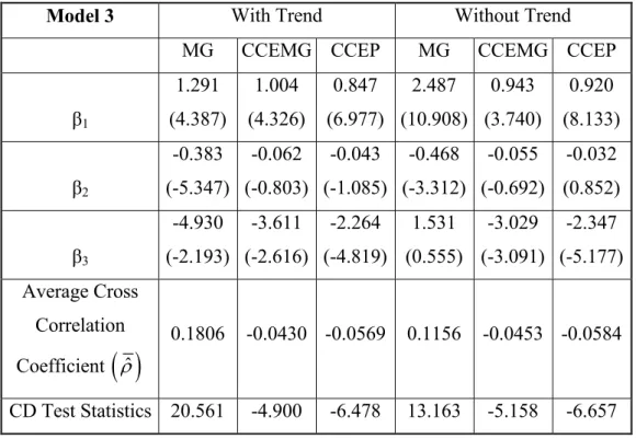
In Model 3, we use first type of volatility as an explanatory variable and total trade flows between the countries in the whole panel as the dependent variable. The results we obtained support the previous results in the literature. The coefficients obtained by using three different estimation methods are -4.930, -3.611 and -2.264 and their respective t-values are -2.193, -2.616 and -4819. As we see from the estimates of the coefficients and their t-values, the effect of developing countries’ exchange rate volatility to their trade flows highly significant in the long run, and the coefficients are greater. For instance one unit increase in the volatility of the exchange rate of a developing country will cause 3.611 percent decrease in the trade flows of that country in the long run if we consider the CCEMG estimator. This empirical evidence shows us that the trade flows of the developing countries are significantly negatively affected from the changes in the volatility of their exchange rates.

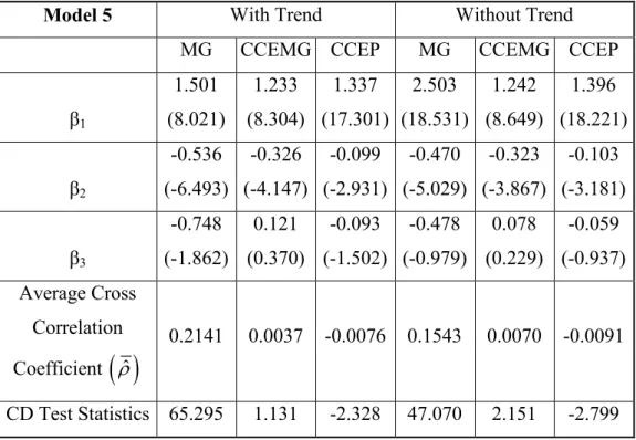
In Models 4 and 5 we use total world trade of the countries instead of the total trade flows of the countries within the panel. The long-run estimations give similar results to the Models 1 and 2. The coefficients of the volatility for Model 4 are -4.409, -2.719 and -0.324 and their t-values are -1.684, -1.100 and -2.419 respectively. As we see from the results the significance and the size of the coefficients are sensitive to the estimation methods we use. The estimates obtained by MG and CCEMG are insignificant, while the estimates obtained by using CCEP is significant. For Model 5, 0.748, 0.121 and -0.093 are the estimated coefficients of Model 5, and -1.862, 0.370 and -1.502 are the respective t-values. In this case the estimated coefficients are all insignificant. And interestingly the estimated coefficient of CCEMG procedure is positive.

30

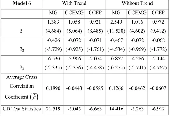
The long run estimation results of the 6th Model are similar to the results for the 3rd Model. The estimated coefficients are 6.530, 3.906, 2.074 and their tvalues are -2.335, -2.376, -4.478 respectively. If we consider the only valid estimation method CCEMG results; we can claim that in the long-run one unit increase in the volatility will cause 3.906 percent decrease in the trade flows.

31

Section 8

Conclusion

In this study we examined the effect of exchange rate volatility to the trade flows by using two different country sets. One is a set of 42 heterogeneous countries, the other one is a set of 16 developing countries. We used panel data approach to the issue. We used unit root tests and long-run estimation methods which allow for cross section dependence. The long run estimation results showed us that, there is no significant effect of exchange rate volatility to the trade flows in the case of 42 heterogeneous countries. But the effect is significant in the case of 16 developing countries. In the light of these results we can conclude that the trade flows developing countries are more affected from the exchange rate volatility than developed countries. The long-run results we obtained is consistent with the empirical results of Doganlar (2002) and Grier and Smallwood (2007). This study can be extended by using different trade flow demand models. For instance the gravity model can be used to explain the trade flow demand. Another aspect of the study which can be extended is the measure we used for the volatility of the exchange rate. GARCH model can be used to measure the volatility of the exchange rate.

32

Appendix: Tables

Table 1: Residual Cross Correlation of ADF(p) Regressions1

Average Cross Correlation Coefficients

ADF(1) ADF(2) ADF(3) ADF(4)

Trade Flows ( )tf _{0.349 0.292 0.292 0.289} Gdp ( )y _{0.062 0.059 0.057 0.062} Exchange Rates ( )e _{0.243 0.232 0.233 0.231} Volatility 1 (( )v _{1 0.126 0.11 0.106 0.099} Volatility 2 ( )v _{2 0.086 0.084 0.084 0.08} World Trade (wt ) _{0.368 0.303 0.305 0.301} Trade Flows (D) (tfd) _{0.237 0.224 0.226 0.214} Gdp (D) ( d) y _{0.037 0.035 0.036 0.044} Exchange Rates (D) ( d) e _{0.089 0.089 0.092 0.091} Volatility 1 (D) (v₁d) _{0.019 0.022 0.014 0.011} World Trade (D) (wtd) _{0.254 0.234 0.241 0.229} 1

Pth-order Augmented Dickey-Fuller test statistics, ADF(p), for trade volume, GDP, population, RLF, SIM, volatility and exchange rates are computed for each cross section unit separately. An intercept and a linear time trend are included in the ADF(p) regressions. The values in “Average Cross Correlation Coefficients” are the simple average of the pair-wise cross section correlation coefficients of the ADF(p)

regression residuals.

[

]

1 1 1 ˆ 2 ( 1) ˆ N N it i j i N N ρ ρ − = = +

= −

∑ ∑

with

ρ

ˆ_it being the correlation coefficient of the ADF(p) regression between the i th and j th cross section units.