Effect of different network geometry on GNSS results

EFFECT OF DIFFERENT NETWORK GEOMETRY ON GNSS RESULTS

Shamal Fatah Ahmed AHMED1_{, Ramazan Alpay ABBAK}2

1_{Department of Geomatics Engineering, Selcuk University, Konya Turkey} 2_{Department of Geomatics Engineering, Selcuk University, Konya Turkey}

shamalsurvey@gmail.com, aabbak@selcuk.edu.tr Abstract

Global Navigation Satellite System (GNSS) is mostly used to establish geodetic networks in surveying engineering. To establish a geodetic network, one should have an understanding of the various types of geodetic networks, their design, accuracy requirements, and essence. The main area where GNSS networks are needed include mapping, tracking crustal movements, planning large engineering projects, implementing cadastral works, designing urbanization activities, GIS, etc. In GNSS network, stations are generally located where they are needed, but the observation schema between stations are important. The main goal of this research was to select the best observation schema of GNSS networks according to the number of receivers and the redundancy of the observation. In this research, six points were established after reconnaissance the field of the project. After preparation the sessions according to the number of receivers, time, and distance between points observations were made by using static method. Data collections were made by using two and three receivers. From data collected in three days four types of geometric design of GNSS network were selected. The first was Hub method that is from one fixed point the new points (i.e. six points in this study) were observed. The second one was Star method that is one fixed point in the center of the new network and observed unknown points. The third was Loop method 1 (using two receivers) where all baselines (i.e. 21 baselines in this study) were observed from one known point and the last was Loop method 2 (using three receivers) from one fixed point. These methods had some advantage and disadvantage according to the type of the project that are selected. Due to no redundancy, no close loop, and no nontrivial line between adjacent points the first and

second methods are not recommended for the establishment of the precise GNSS network in our study.

Keywords: GNSS network design, Redundancy, Static method, Session.

FARKLI AĞ GEOMETRİSİNİN GNSS SONUÇLARINA ETKİSİ

Özet

GNSS (Global Navigation Satellite System) arazi ölçmelerinde jeodezik ağların kurulmasında sıkça kullanılır. Bir jeodezik ağı kurmak için, ağın türünü, tasarımını, doğruluk isteklerini bilmek gerekir. GNSS ağının ihtiyaç olduğu alanlar; haritalama, yer kabuğu hareketlerinin izlenmesi, geniş çaplı mühendislik projelerinin planlanması, kadastral çalışmalarının uygulanması ve CBS aktivitelerini içerir. GNSS ağında, noktalar nerede ihtiyaç duyulursa orada tesis edilir. Fakat noktalar arasındaki gözlem şeması önemlidir. Bu çalışmanın ana amacı; fazla gözlem sayısı ve alıcı sayısı düşünülerek GNSS ağında en uygun ölçü tasarımını belirlemektir. Bu kapsamda proje sahasında 6 nokta tesis edilmiştir. Oturumlar hazırlandıktan sonra, alıcı sayısı, noktalar arası uzaklık ve zaman göz önünde bulundurularak statik ölçüler gerçekleştirilmiştir. 3 günlük veri toplama sürecinde GNSS ağının farklı 4 çeşit ağ tasarımı denenmiştir. Veri toplama sürecinde iki ve üç alıcı kullanılmıştır. Birincisi bir sabit noktadan yeni noktalara ölçü yapan Hub metodudur (yeni nokta sayısı 6 dır). İkincisi ağın merkezindeki bir noktayı sabit alıp diğer noktaları gözlemleyen Star yöntemidir. Üçüncüsü bilinen bir noktadan tüm noktaların gözlemlendiği iki alıcılı Loop yöntemidir. Sonuncusu iki sabit noktalı ve üç alıcılı Loop yöntemidir. Seçilen projelerin türüne göre yöntemlerin üstünlükleri ve zayıflıkları bulunmaktadır. Sayısal sonuçlara göre fazla ölçü sayısındaki eksiklik ve kapalı lupların olmaması nedeniyle birinci ve ikinci yöntem, yüksek duyarlıklı GNSS ağ tasarımında tavsiye edilmez.

1. Introduction

Locating points of interest on the earth’s surface is the specialty of surveying. The locations of points of interest are defined by coordinate values that are referenced to a predefined mathematical surface. In geodetic surveying, datum is this mathematical surface, and its coordinates define the position of a point with respect to the datum. The reference surface for a system of control points is identified by its position with respect to the shape and size of the earth. A datum is a coordinate surface used as reference figure for positioning control points. Control points are points with known relative positions tied together in a network [14]. To establish a geodetic network, one must have an understanding of the various types of geodetic networks, their design, essence and accuracy requirements [14]. There are three basic kinds of geodetic control: Vertical, Horizontal and Gravity [13].

This research will focus on horizontal control, that is a network of stations of known grid or geographic positions referred to as a common horizontal datum, which control the horizontal positions of mapped features corresponding to latitude and longitude, or easting and northing grid lines displayed on the map [4]. Field procedures used in horizontal control surveys have traditionally been the ground methods of trilateration, precise traversing, triangulation and combinations of these basic methods. Satellite surveying has been employed with increasing frequency, especially in control surveys. Due to some advantage including its speed, easy use, and extremely high accuracy abilities over long distances GNSS surveys are rapidly replacing the basic methods.

In this research it is discussed about four types of GNSS network design (i.e. Hub, Star, Loop method 1 (using two receivers) and Loop method 2 (using three receivers). [3] describes two types of GNSS network design theoretically as Hub and Loop method from one fixed point. Also it presents the advantages and disadvantages of them. But this study numerically describes the four types and comparison between them based on the standard deviation of coordinates and the position quality of points as well.

The paper started with the general principle of GNSS surveying with the static method and observation schema. Then the data collection strategy was discussed in the test

area. Accuracies of the four types of GNSS network were analyzed in the test area. Finally results of this research were summarized in the last section.

2. Method

GNSS field procedures working on surveys depend on the abilities of the kind of survey and the receivers. Currently some specific field procedures being used in surveying consist of the pseudo-kinematic, kinematic, static and rapid static methods. All are based on carrier phase-shift measurements and employ relative positioning techniques; that is, two (or more) receivers, occupying different stations and at the same time making observations to the same satellites. Baseline is the distance between receivers, and its , , and coordinate difference components are computed as a result of the observations [7].

Figure 1. Static GNSS surveying [5]

Since static method was used in the current research, the method is briefly described as follows: static GNSS surveying is a relative positioning technique that depends on the carrier-phase measurements [5]. In geodetic control surveys this method is used to provide high precision over long baselines [9]. It works two (or more) stationary receivers all together tracking the same satellites (Fig. 1). One receiver, the base receiver, is set up over a point with precisely known coordinates such as a survey monument (sometimes referred to as the known point). The other receiver, the remote receiver, is set up over a point whose

coordinates are unknown. The base receiver can support any number of remote receivers, as long as a minimum of four common satellites is visible at both the base and the remote sites [5].

After establishment the stations, for execution the work an observation scheme is developed. The scheme consists of a planned sequence of observing sessions that accomplishes the objectives of the survey in the most efficient manner. However, some redundant observations should be including in the plan (i.e. repeat observations of some baselines, baseline observations between fixed points and multiple occupations of stations) to be used for checking purposes, and for improving the precision and reliability of the work. For any observing session in relative positioning, the number of nontrivial baselines measured is the number of receivers used in the session minus one, or

b = r-1 (1)

where b is the number of nontrivial baselines and r the number of receivers being employed in the session. When in a session only two receivers are used, only one baseline is observed and it is nontrivial. If three or more receivers are used, both trivial (mathematically dependent) and nontrivial baselines will result. In practice, in a four-receiver session the three shortest lines are almost always supposed the independent baselines, and the three longest baselines are deleted as trivial or dependent.

If only two receivers were used there would be no trivial lines and it might seem there would be no redundancy at all. However, to connect each station with its nearest neighbor, each station would have to be occupied at least twice, and each time during a different session [6, 12]. One option is to operate one instrument at a central station, and occupy the adjacent points in a star-shaped pattern. Adjacent central stations are linked through baseline observations. Another possibility is to occupy neighboring points and form triangles or quadrangles. This method leads to a high relative accuracy [10].

The stations are connected through non trivial baselines in the form of loop if more than two receivers were used. For control surveys, due to necessary to perform closure checks the baselines should form closed geometric figures [7].

First-order, second-order, and third-order GNSS control networks shall be designed with adequate redundancy to detect and isolate systematic errors and/or blunders.

Redundancy of network design is achieved by many way is different from one author to another; for example, related to [8], the highest accuracy and reliability of a GNSS network are anticipated if all the possible combinations of baselines in the network would be observed. Related to the [11] to provide order AA geometric accuracy standards, the FGCC requires three or more occupations on 80% of the stations in a project. Three or more occupations are necessary on 40%, 20%, and 10% of the stations for A, B, and C standards, respectively. When the distance between a station and its azimuth mark is less than 2 km, both points must be occupied at least twice to meet any standard above second-order. Two or more occupations are required for all horizontal control stations in order AA—the percentage requirements for repeat occupations on horizontal control stations drops to 75%, 50%, and 25% for A, B, and C, respectively. [2] says that the redundancy of network design is achieved by:

• Repeat baseline observations

• Attaching each network station through at least two non-trivial baselines • Series of interconnecting, closed loops

3. Numerical Application

3.1 Study Area

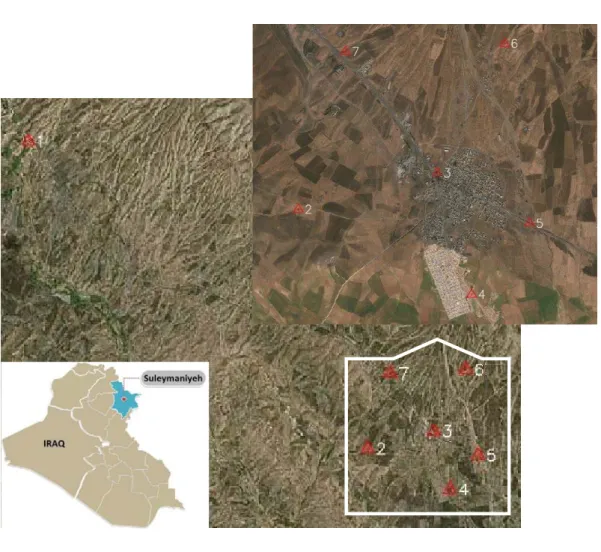
The location of the project was in the Suleymaniyeh city in Iraq at latitude and longitude 35°30’ 44” and 45° 26’ 26” respectively. After determination of the location of six points on an aerial photo (Fig. 2), the field was visited to check the location of the points. After reconnaissance the field, the points were monumented as three-dimensional monument.

3.2. GNSS Data

According to the number of receivers, the distance between points and time by using static method [7], the sessions were prepared. The first and second day by using two Leica GS15 (Dual frequency and GNSS type: GPS and GLONASS) receivers and one fixed point (i.e. point no.1) the sessions were prepared (Table 1). In the third day by using the same receivers plus one Leica 1200 (Dual frequency and GNSS type: GPS) receiver with the same fixed point, the sessions were prepared (Table 2).

Figure 2. Study area

Table 1. Sessions for first and second day using two receivers Sessions From To Distance

(km) Occupation time (min) 1 1 2 14.42 90 First 2 1 3 15.69 90 Day 3 1 4 17.21 90 4 1 5 17.25 90 5 1 6 15.56 90 6 1 7 13.56 90 7 2 3 2.15 30  

8 2 4 2.98 30 9 2 5 3.54 30 10 2 6 3.97 30 11 2 7 2.48 30 12 3 4 1.98 30 Second 13 3 5 1.68 30 Day 14 3 6 2.2 30 15 3 7 2.30 30 16 4 5 1.37 30 17 4 6 3.88 30 18 4 7 4.20 30 19 5 6 2.83 30 20 5 7 3.88 30 21 6 7 2.39 30

Table 2. Sessions for third day using three receivers

3.3. Results

Before data collection, mission planning was made through GNSS Planning Online – Trimble tool in the Trimble website to check the best time for observation. From the collected data four types of network design were selected for evaluation and comparison between them, and also for deciding of what the advantages and disadvantages are and

Sessions Stations Occupation time (min) Third 2 1,6,2 90 Day 3 2,6,7 30 4 2,6,3 30 5 6,3,5 30 6 5,3,4 30 7 3,4,2 30 8 3,2,7 30

which one of them is the most economic. For post-processing of this project’s data Leica Geo Office (version 7.0) used and selected processing parameters are shown in Table 3. From the elements of the variance-covariance matrix of the horizontal coordinates of any point, standard deviations of easting, northing, and position quality was determined.

Variance-covariance matrix,

(2) Standard deviation of easting coordinate,

= (3) Standard deviation of northing coordinate,

= (4) Position quality of coordinates,

(5) Table 3. selected processing parameters for post processing

Parameters Selected

Cut-off angle: 15°

Ephemeris type: Precise

Solution type: Automatic

GNSS type: Automatic

Frequency: Automatic

Fix ambiguities up to: 80 km

Min. duration for float solution (static): 5' 00"

Sampling rate: Use all

Tropospheric model: Hopfield

Ionospheric model: Automatic

Use stochastic modelling: Yes

Min. distance: 8 km

The first method was known as Hub (Fig. 3), from one fixed point baselines were observed between new points (i.e. 1-2, 1-3, 1-4, 1-5, 1-6, 1-7), one time without redundancy. The horizontal coordinates standard deviation of easting and northing, and position quality of points presented in Table 4.

Table 4. Hub method, coordinates, standard deviation of easting, northing and position quality [m]

No. Easting Northing

2 550628.4640 3920271.585 0.00254 0.00262 0.00365 3 552743.7675 3920661.510 0.00429 0.00487 0.00649 4 553233.5322 3918996.446 0.00346 0.00394 0.00525 5 554054.3548 3920079.860 0.00324 0.00397 0.00512 6 553728.9814 3922763.425 0.00261 0.00263 0.00371 7 551339.3756 3922641.876 0.00164 0.00217 0.00271

Figure 3. Hub method

The advantages of this type of design are as follows: maintains precision of GNSS observations (i.e. in millimeter see Table 4) and processing software may be able to leverage short and long lines to improve atmospheric modeling.

Disadvantages: Distortions in the local geodetic control system must be rigorously modeled to avoid depositing in vectors adjusted back to the hub(s). Network constraints demand analysis that was more rigorous. Edge matching to adjoining networks was more challenging. Due to no redundancy and loop, the results were not guaranteed because it could not be checked.

The second method was known as Star. In this method, one point in the center of the network (i.e. point number 3) was fixed then the other points (i.e. point number 2, 4, 5, 6, 7) observed one time without redundancy (Fig. 4). The horizontal coordinates, standard deviation of easting and northing, and position quality of points were tabulated in Table 5.

Table 5. Star method, coordinates, standard deviation of easting and northing, and position quality [m]

No. Easting Northing

2 550628.4808 3920271.562 0.00226 0.00221 0.00317 4 553233.5473 3918996.421 0.00428 0.00410 0.00593 5 554054.3807 3920079.836 0.00252 0.00312 0.00401 6 553729.0124 3922763.410 0.00167 0.00208 0.00267 7 551339.4068 3922641.860 0.00249 0.00298 0.00388

The advantages of this type of design are as follows: maintains precision of GNSS observations and processing software may be able to leverage short and long lines to improve atmospheric modeling. The distance between fixed point and unknown points is short; the ambiguity resolution works best over short distances. The occupation time is short, so this method is economic.

Disadvantages: distortions in the local geodetic control system must be rigorously modeled. Network constraints demand more analysis that is rigorous. Edge matching to adjoining networks is more challenging. Due to no redundancy and loop, the results were not still guaranteed because it could not be checked.

The third method is Loop method 1(using two receivers). In this method, one point was fixed (i.e. point number 1) and all baselines in the network (i.e. 21 baselines) were observed (Fig. 5). While free adjustment was performed, 3 baselines were removed. The horizontal coordinates, standard deviation of easting and northing, and position quality of points were shown in Table 6.

Advantages of this type of design are as follows: loop closures provide significant sub-network analysis tool, network diagrams appear more rigorous and can be useful to distribute distortions in the local geodetic control system. Due to more number of baselines, if at the stage of free adjustment some baseline maybe deleted was not a problem. Two receivers were used therefore it is economical. Analysis of loop closures can be done.

Figure 5. Loop method 1 (Black lines are deleted baselines)

Table 6. Loop method 1, coordinates, standard deviation of easting and northing, and position quality [m]

No. Easting Northing

2 550628.4603 3920271.588 0.00335 0.00373 0.00501 3 552743.7410 3920661.531 0.00371 0.00427 0.00565 4 553233.5208 3918996.441 0.00307 0.00348 0.00464 5 554054.3523 3920079.854 0.00322 0.00370 0.00491 6 553728.9848 3922763.430 0.00306 0.00350 0.00465 7 551339.3793 3922641.875 0.00294 0.00353 0.00460 Disadvantages: imposes artificial correlations between observations, losses precision to increase assessment of adjacent stations and for observation of all baselines with two receivers more time is required.

The forth method was Loop method 2 (using three receivers). In this method there were 3 receivers with one known point (Fig. 6). From known point (i.e. point number 1) observations were made according to the Table 2. Because of the receiver 1200 tracked only GPS satellites, therefore all data were processed according to GPS satellites. When

three receivers used, it has one trivial and two non-trivial baselines. Trivial baselines must be deleted before final adjustment. In this type of design, stations were observed at least twice and some of the baselines are observed more than one time. At the result of the free adjustment, one baseline was deleted. The horizontal coordinate, standard deviation of

easting and northing, and position quality of points were given in Table 7.

Table 7. Loop method 2, coordinates, standard deviation of easting and northing, and position quality [m]

No. Easting Northing

2 550628.4616 3920271.585 0.00344 0.00375 0.00509 3 552743.7428 3920661.527 0.00385 0.00429 0.00577 4 553233.5236 3918996.438 0.00379 0.00422 0.00567 5 554054.3540 3920079.851 0.00369 0.00419 0.00558 6 553728.9859 3922763.427 0.00340 0.00363 0.00497 7 551339.3770 3922641.865 0.00402 0.00458 0.00609

Advantages of this type of design are as follows: loop closures provide significant sub-network analysis tool, network diagrams appear more rigorous and can be useful to distribute distortions in the local geodetic control system. In this method, some analysis may be performed like analysis of repeat baseline measurements and analysis of loop closures.

Disadvantages: imposes artificial correlations between observations and losses precision to increase assessment of adjacent stations.

According to the position quality of points, the results were more accurate in all methods, but due to no redundancy and no loop, the stations cannot be checked, so the first and second methods (i.e. Hub and Star) are refused. The other methods (i.e. Loop method 1 and Loop method 2) are recommended for establishing geodetic network in our study due to redundancy and close loop (Table 8, Figure 7a and b).

Table 8. Comparison of methods according to the position quality No. (hub) (star) (loop method 1) (loop method 2)

2 0.00365 0.00317 0.00501 0.00509 3 0.00649 0 0.00565 0.00577 4 0.00525 0.00593 0.00464 0.00567 5 0.00512 0.00401 0.00491 0.00558 6 0.00371 0.00267 0.00465 0.00497 7 0.00271 0.00388 0.00460 0.00609

Figure 7a. Comparison of position quality of points according to methods.

Figure 7b. Comparison of position quality of methods according to the points

4. Conclusion

In the establishment of any GNSS network before starting data collection, the design of network (i.e. the scheme of the observation) should be realized according to the number of receivers, redundancy, and desired accuracy. In GNSS networks the location of points are not important, but the observation schema is important. Network observation design helps identify and remove blunders in network surveying. It also ensures that the

0 0,002 0,004 0,006 0,008 2 3 4 5 6 7 st anda rd d ev ia tion [m ]

Comparison

positon quality(hub) positon quality(star)

positon quality(loop method 1) positon quality(loop method 2)

0 0,001 0,002 0,003 0,004 0,005 0,006 0,007 positon

quality(hub) positon quality(star) positon quality(loopmethod 1) positon quality(loopmethod 2)

st andard d ev ia tion [m]

comparison

impact of undetected and unremoved errors is minimal in network solutions. It also used to reduce the time and effort required to perform field projects and reduce project costs.

In this research, from the collected data in three days, four types network design were selected for evaluation and comparison between them, and also for deciding of what the advantages and disadvantages are and which one of them was the most economic. Therefore, the result of this research was indicated that, when the number of baseline increased the accuracy of network automatically increased because at the stage of free adjustment some baseline may be deleted due to errors. In this research, the first and second method were not recommended because there was no redundancy and no loop. However, the third method (i.e. Loop method 1using two receivers) and forth method (i.e. Loop method 2 using three receivers) were recommended because there was redundancy, closed loop, and multi occupation points.

According to this research some general guidelines can be suggested:

 To detect blunders, all stations should be set up at least twice, in different conditions,

 Linking all network stations with two or more nontrivial baselines,

 Adjacent stations should be set up at the same time as the ambiguity solving works best over short distances, and

 For accuracy checks some of baselines should be observed double. References

[1] Bundoo, C. S. (2013). Establishing A Geodetic Reference Network In Montserrado County – Liberia Using GNSS Technology, Kwame Nkrumah University of Science and Technology, Ghana.

[2] CDT, California Department Of Transportation (2006). Caltrans Surveys Manual. California.

[3] CLSA and CSRC, California Land Surveyors Association And California Spatial Reference Center (2014). GNSS Surveying Standards And Specifications. California.

[4] DMATC, Defense Mapping Agency Topographic Center (1973). Defense Of Mapping, Charting, And Geodetic Terms, Ntis National Techincal Information Services, U. S. Department Of Commerce, Washington.

[5] El-Rabbany, A. (2002). Introduction To GPS, The Global Positioning System, Artech House, USA.

[6] FGCC (1988). Geometric Geodetic Accuracy Standards And Specifications For Using GPS Relative Positioning Technique, Rockville, Maryland.

[7] Ghilani, C. D., & Wolf, P. R. (2015). Elementary Surveying An Introduction To Geomatics, Pearson, USA.

[8] Kuang, S. (1996). Geodetic Network Analysis And Optimal Design: Concepts And Applications. Ann Arbor Press, Michigan.

[9] Schofield, W., & Breach, M. (2007). Engineering Surveying. Elsevier, UK. [10] Seeber, G. (2003). Satellite Geodesy. Walter De Gruyter, Berlin.

[11] Sickle, J. V. (2008). GPS For Land Surveyors, Third edition, Crc Press, USA. [12] Sickle, J. V. (2015). GPS For Land Surveyors, Fourth edition, Crc Press, USA. [13] Torge, W. (1991). Geodesy, De Gruyter, Berlin.

[14] USACE, (2002). Geodetic And Control Surveying. Us Army Corps Of Engineers, Washington.